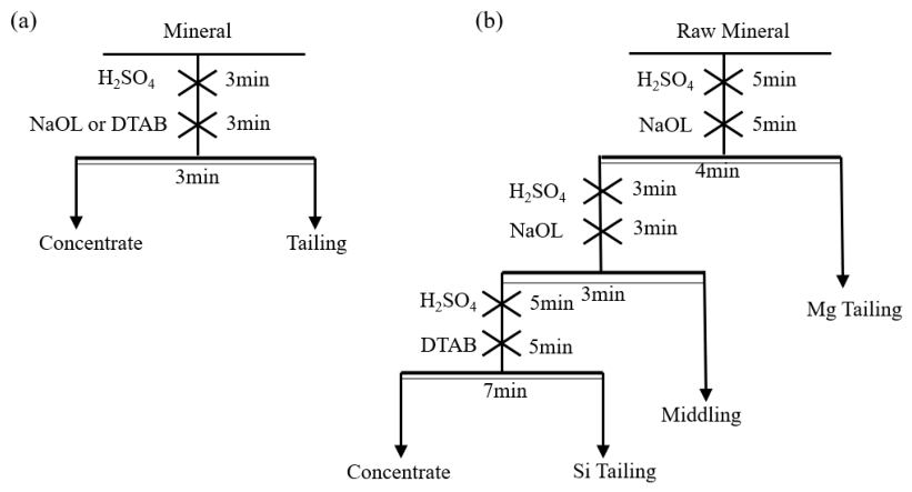
Figure 1.
Schematic Flowsheets of (a) the micro-flotation test and (b) the bench-scale double reverse flotation.
Figure 1.
Schematic Flowsheets of (a) the micro-flotation test and (b) the bench-scale double reverse flotation.
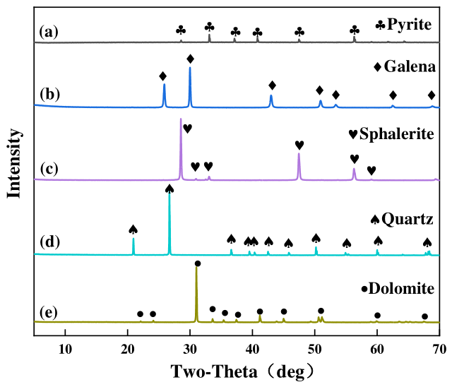
Figure 2.
XRD patterns of the pyrite (a), galena (b), sphalerite (c), quartz (d), and dolomite (e) samples.
Figure 2.
XRD patterns of the pyrite (a), galena (b), sphalerite (c), quartz (d), and dolomite (e) samples.
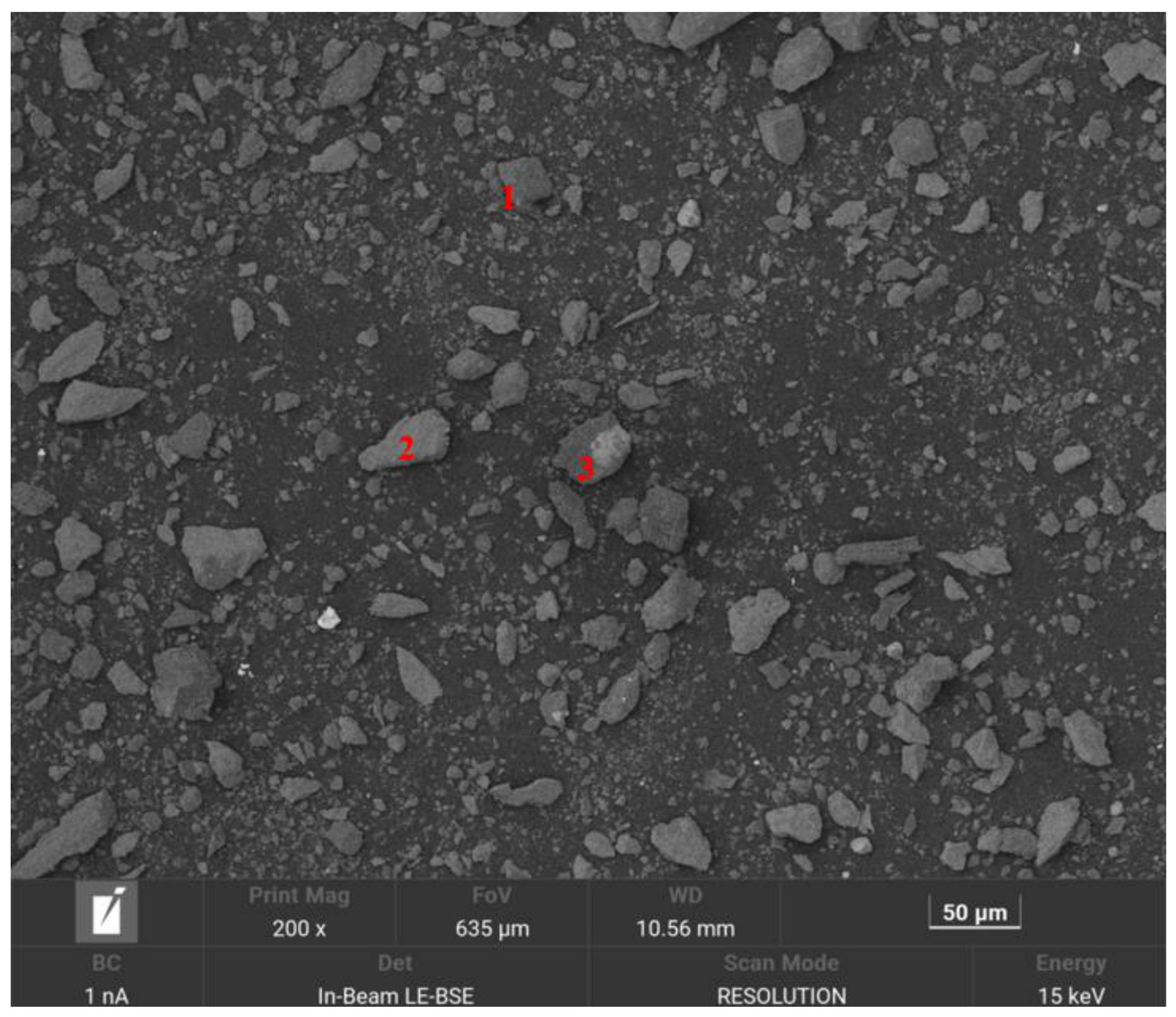
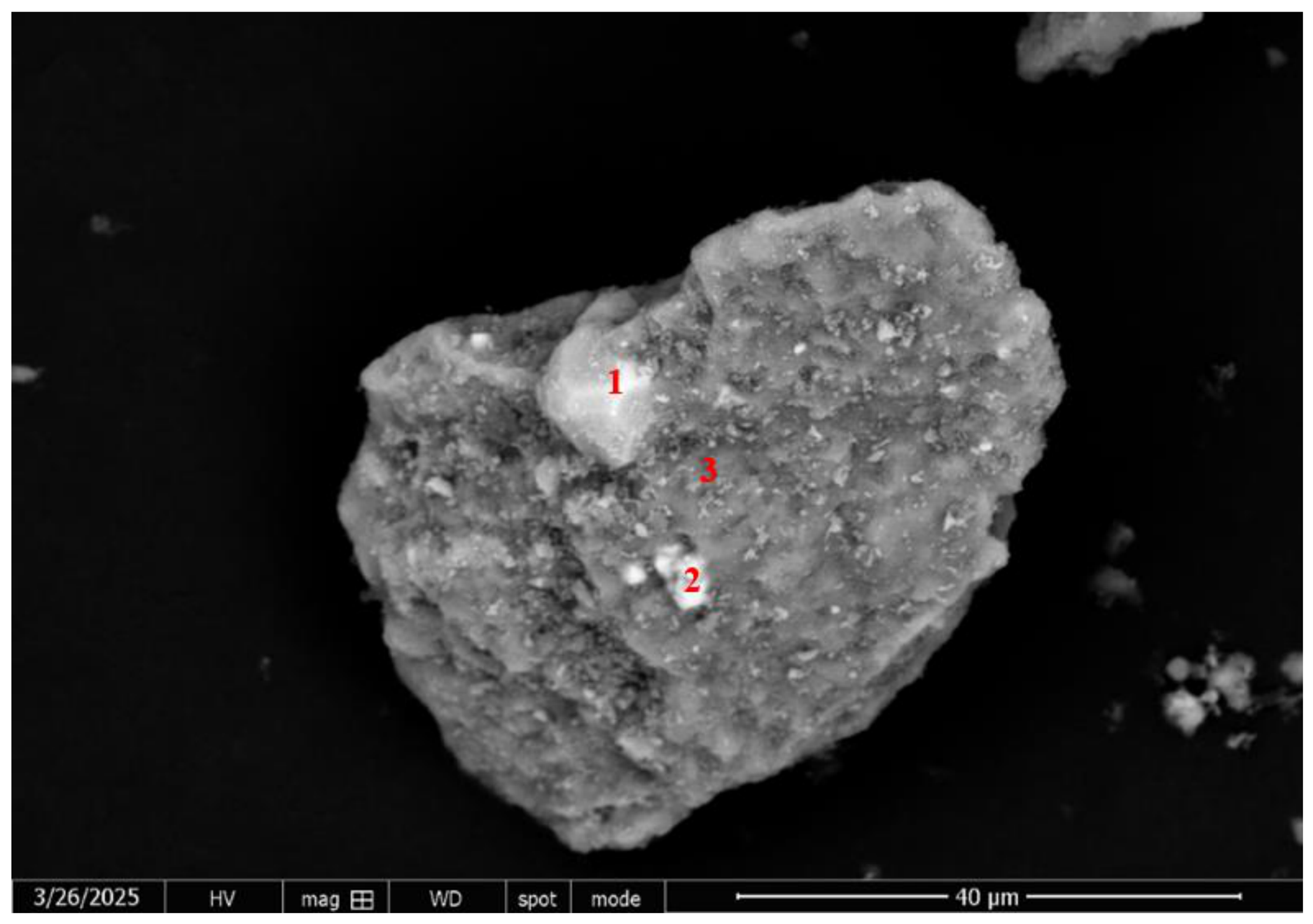
Figure 3.
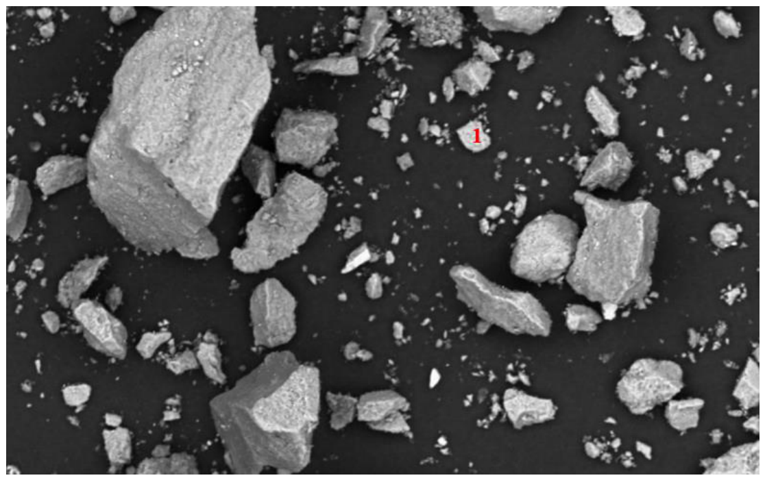
SEM micrograph of the run-of-mine ore. The red numbers (1, 2, and 3) indicate the specific locations of the EDS point analyses corresponding to the data in
Table 1.
Figure 3.
SEM micrograph of the run-of-mine ore. The red numbers (1, 2, and 3) indicate the specific locations of the EDS point analyses corresponding to the data in
Table 1.
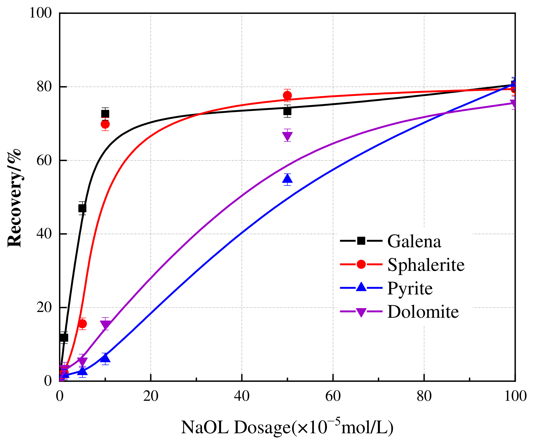
Figure 4.
Effect of NaOL dosage on the flotation recovery of galena, sphalerite, pyrite, and dolomite. The scatter points represent the experimental data, and the solid lines are drawn to guide the eye. Error bars indicate the standard deviation of independent experiments.
Figure 4.
Effect of NaOL dosage on the flotation recovery of galena, sphalerite, pyrite, and dolomite. The scatter points represent the experimental data, and the solid lines are drawn to guide the eye. Error bars indicate the standard deviation of independent experiments.
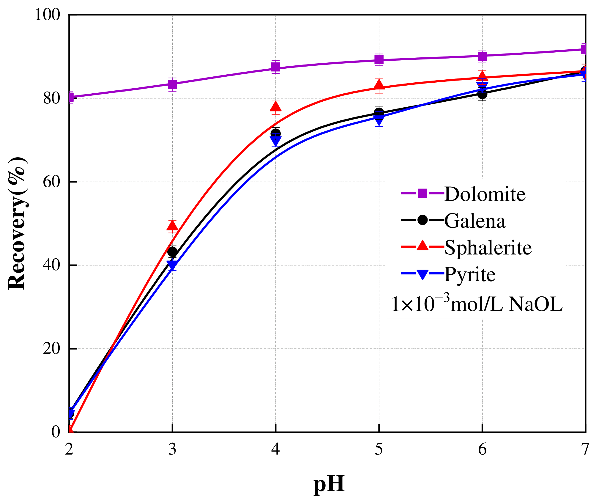
Figure 5.
Effect of various pH on the flotation recovery of galena, sphalerite, pyrite, and dolomite. The scatter points represent the experimental data, and the solid lines are drawn to guide the eye. Error bars indicate the standard deviation of independent experiments.
Figure 5.
Effect of various pH on the flotation recovery of galena, sphalerite, pyrite, and dolomite. The scatter points represent the experimental data, and the solid lines are drawn to guide the eye. Error bars indicate the standard deviation of independent experiments.
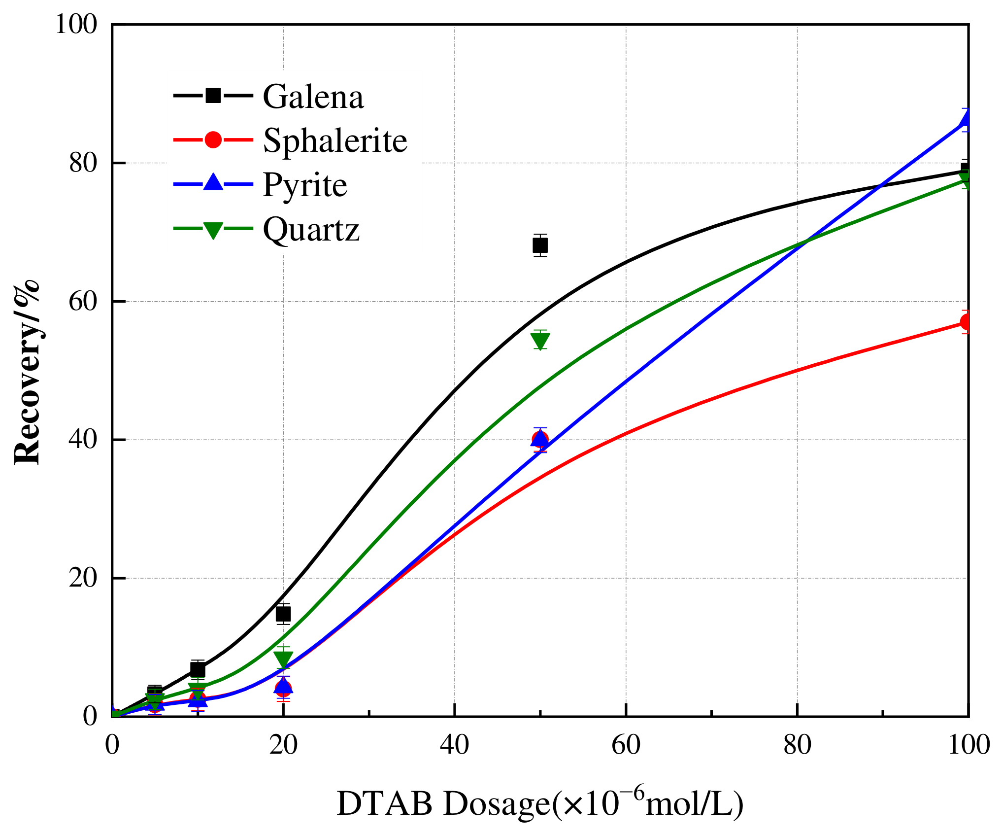
Figure 6.
Effect of DTAB dosage on the flotation recovery of galena, sphalerite, pyrite, and quartz. The scatter points represent the experimental data, and the solid lines are drawn to guide the eye. Error bars indicate the standard deviation of independent experiments.
Figure 6.
Effect of DTAB dosage on the flotation recovery of galena, sphalerite, pyrite, and quartz. The scatter points represent the experimental data, and the solid lines are drawn to guide the eye. Error bars indicate the standard deviation of independent experiments.
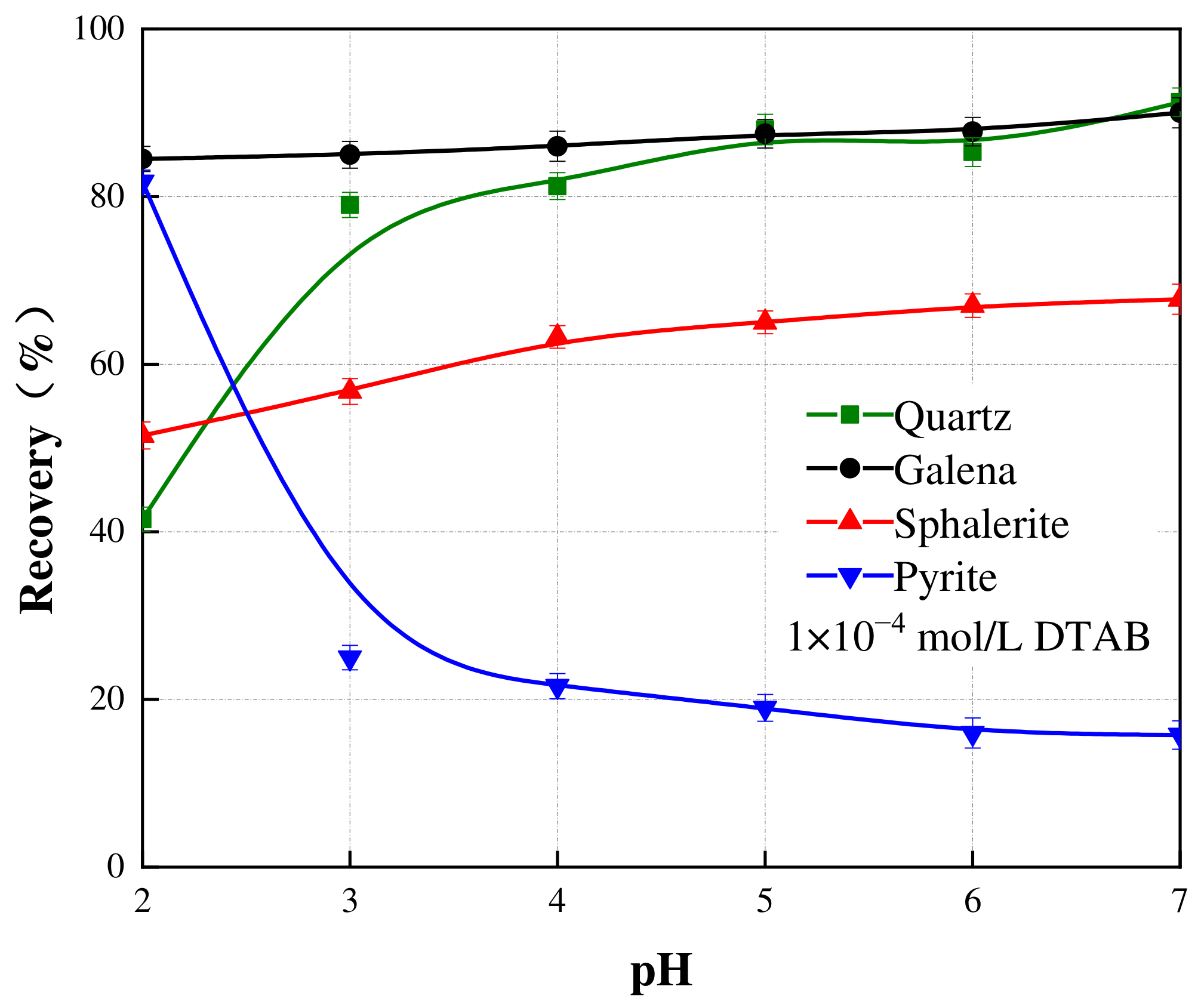
Figure 7.
Effect of various pH on the flotation recovery of galena, sphalerite, pyrite, and quartz. The scatter points represent the experimental data, and the solid lines are drawn to guide the eye. Error bars indicate the standard deviation of independent experiments.
Figure 7.
Effect of various pH on the flotation recovery of galena, sphalerite, pyrite, and quartz. The scatter points represent the experimental data, and the solid lines are drawn to guide the eye. Error bars indicate the standard deviation of independent experiments.
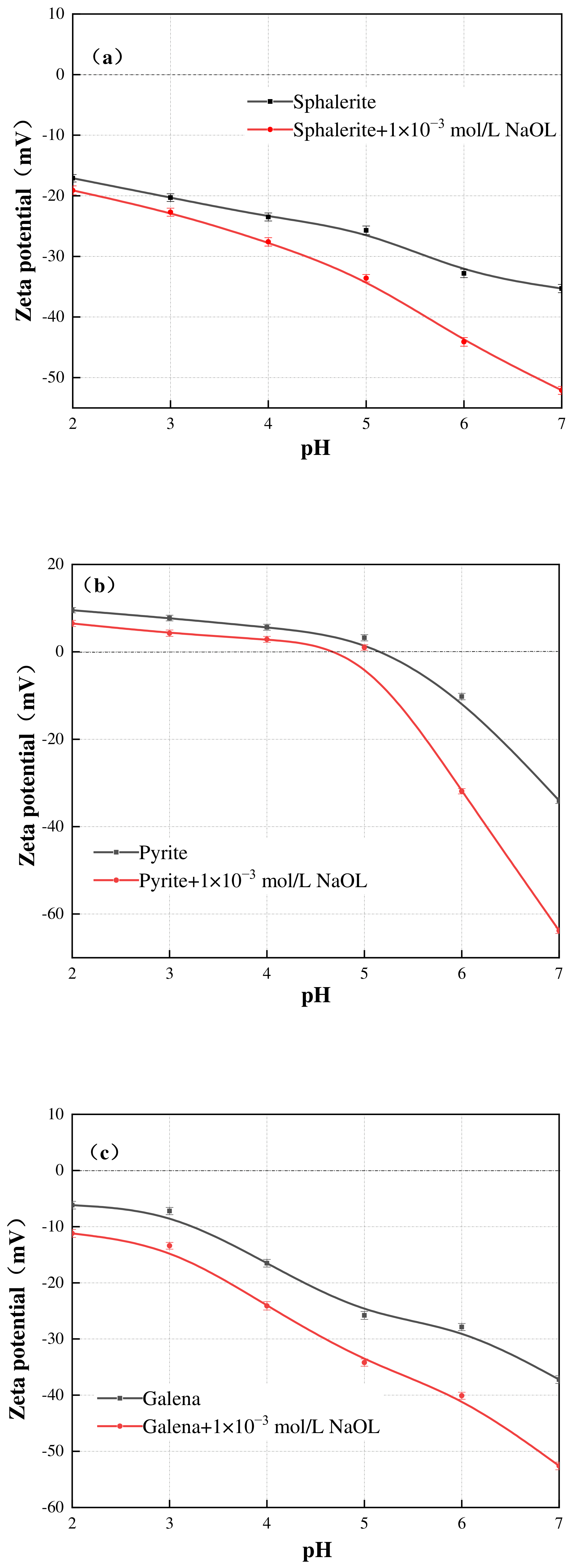
Figure 8.
Zeta potential of sphalerite (a), pyrite (b) and galena (c) at various pH in the NaOL system. The scatter points represent the experimental data, and the solid lines are provided as visual guides. Error bars indicate the standard deviation of independent measurements.
Figure 8.
Zeta potential of sphalerite (a), pyrite (b) and galena (c) at various pH in the NaOL system. The scatter points represent the experimental data, and the solid lines are provided as visual guides. Error bars indicate the standard deviation of independent measurements.
Figure 9.
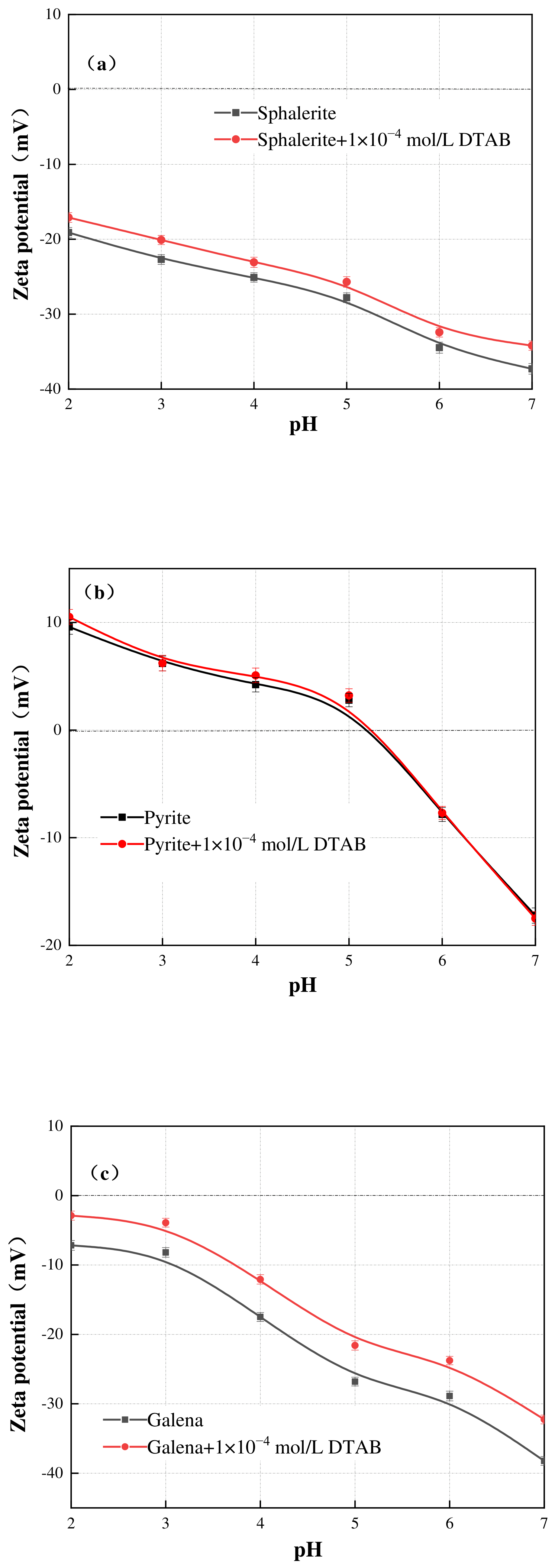
Zeta potential of sphalerite (a), pyrite (b) and galena (c) at various pH in the DTAB system. The scatter points represent the experimental data, and the solid lines are provided as visual guides. Error bars indicate the standard deviation of independent measurements.
Figure 9.
Zeta potential of sphalerite (a), pyrite (b) and galena (c) at various pH in the DTAB system. The scatter points represent the experimental data, and the solid lines are provided as visual guides. Error bars indicate the standard deviation of independent measurements.
Figure 10.
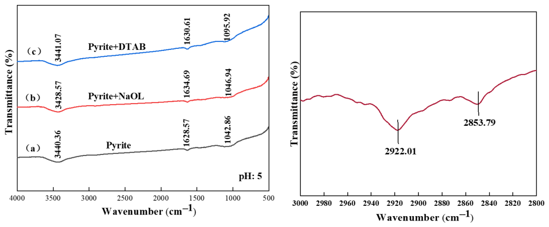
FTIR spectra of pyrite surface: (a) pristine, (b) treated with NaOL, (c) treated with DTAB and the enlarged view of the 3000–2800 cm−1 region for sodium oleate and pyrite.
Figure 10.
FTIR spectra of pyrite surface: (a) pristine, (b) treated with NaOL, (c) treated with DTAB and the enlarged view of the 3000–2800 cm−1 region for sodium oleate and pyrite.
Figure 11.
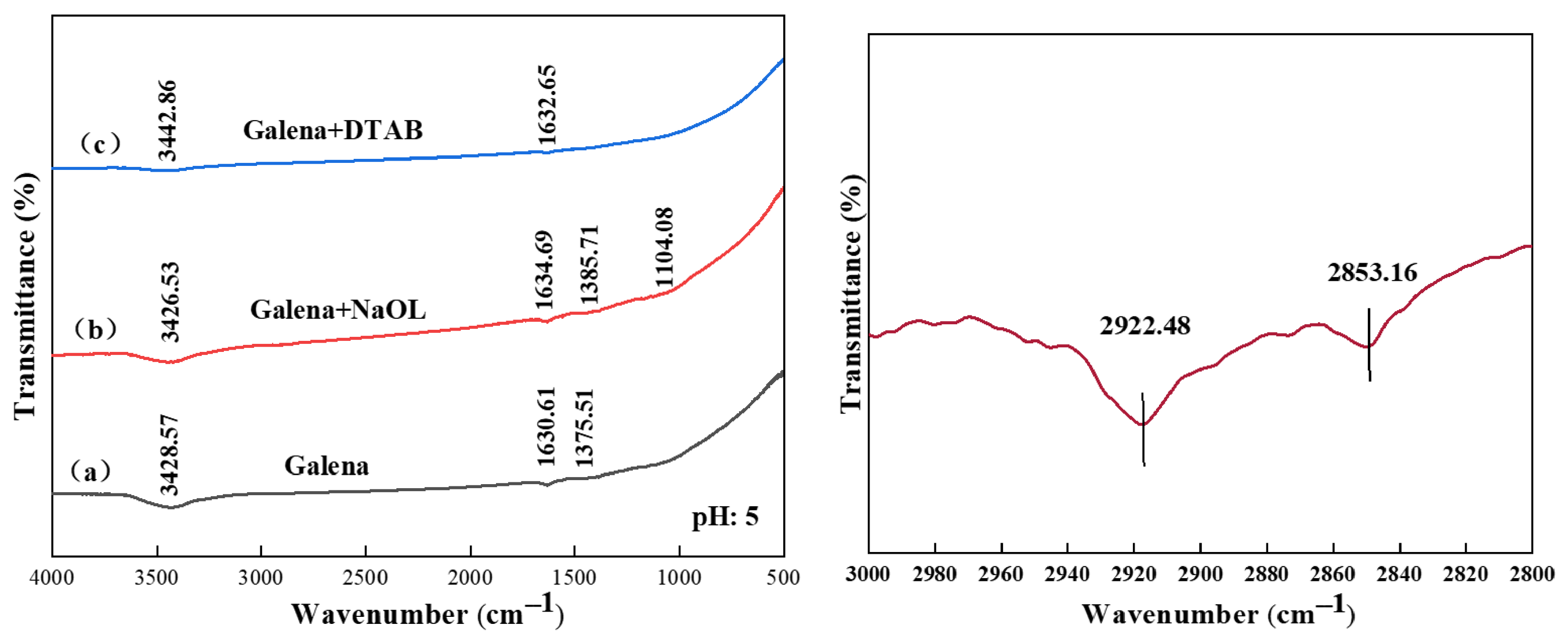
FTIR spectra of galena surface: (a) pristine, (b) treated with NaOL, and (c) treated with DTAB and the enlarged view of the 3000–2800 cm−1 region for sodium oleate and galena.
Figure 11.
FTIR spectra of galena surface: (a) pristine, (b) treated with NaOL, and (c) treated with DTAB and the enlarged view of the 3000–2800 cm−1 region for sodium oleate and galena.
Figure 12.
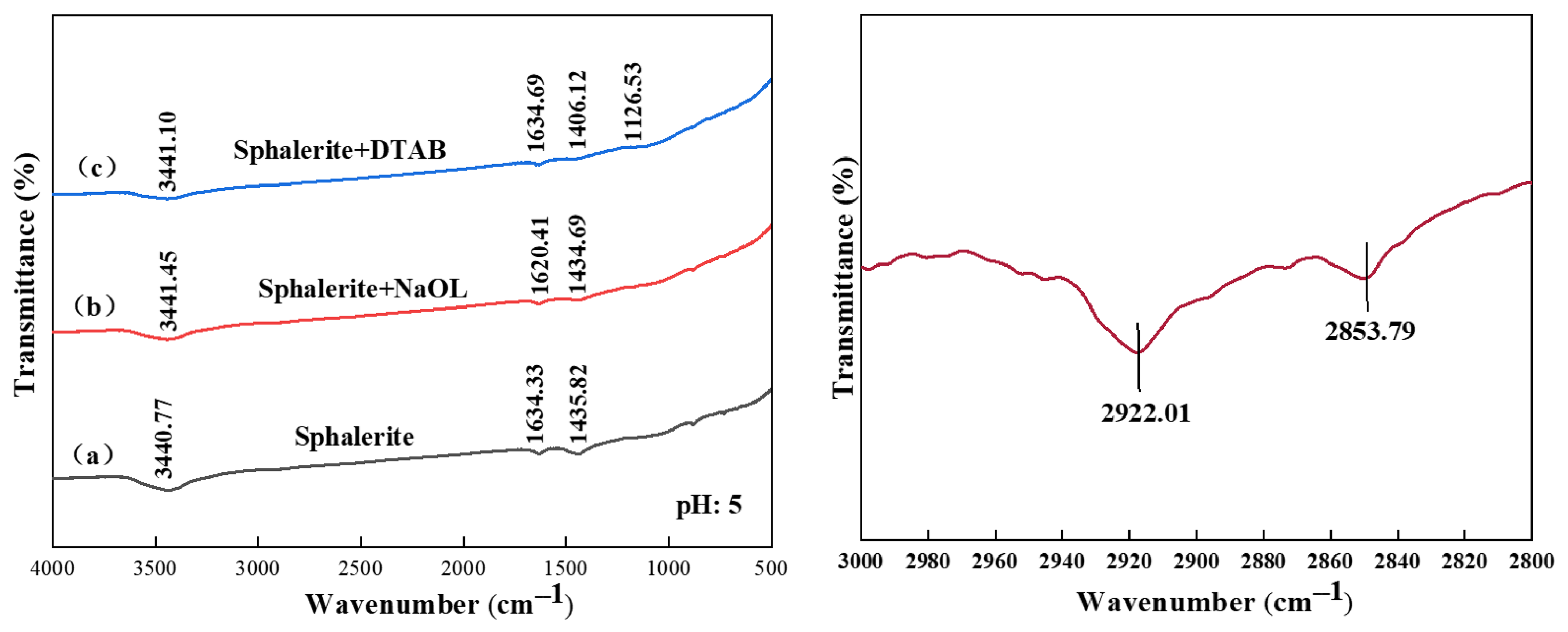
FTIR spectra of sphalerite surface: (a) pristine, (b) treated with NaOL, and (c) treated with DTAB and the enlarged view of the 3000–2800 cm−1 region for sodium oleate and sphalerite.
Figure 12.
FTIR spectra of sphalerite surface: (a) pristine, (b) treated with NaOL, and (c) treated with DTAB and the enlarged view of the 3000–2800 cm−1 region for sodium oleate and sphalerite.
Figure 13.
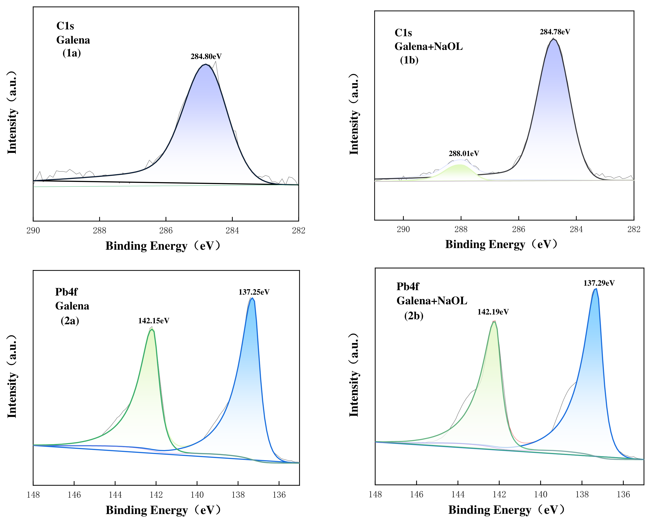
C1s, Pb4f XPS spectra on galena surface untreated (1a,2a), treated with NaOL (1b,2b). The different colored lines and shaded areas represent the deconvoluted component peaks.
Figure 13.
C1s, Pb4f XPS spectra on galena surface untreated (1a,2a), treated with NaOL (1b,2b). The different colored lines and shaded areas represent the deconvoluted component peaks.
Figure 14.
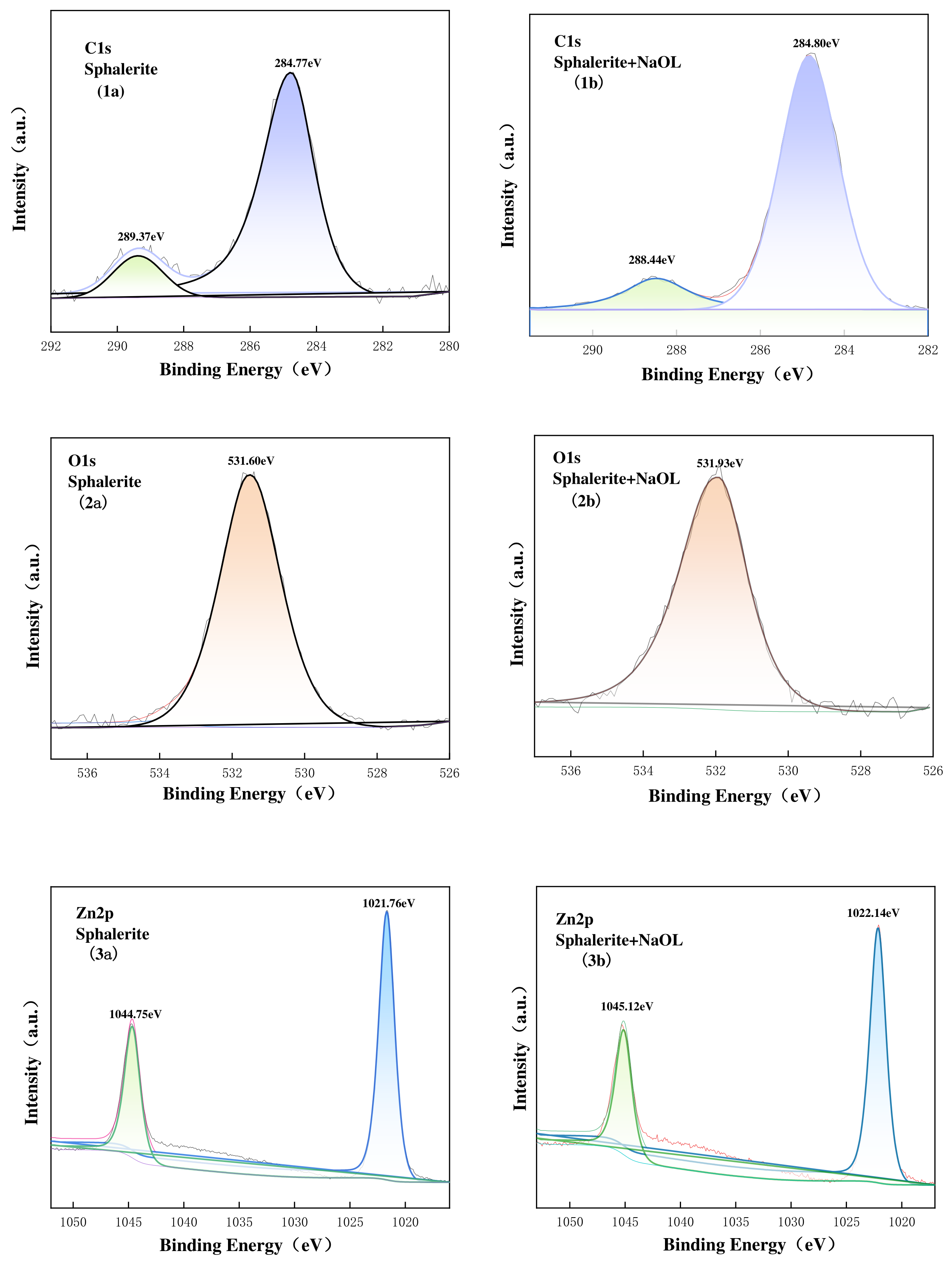
C1s, O1s and Zn2p XPS spectra on sphalerite surface untreated (1a,2a,3a), treated with NaOL (1b,2b,3b). The different colored lines and shaded areas represent the deconvoluted component peaks.
Figure 14.
C1s, O1s and Zn2p XPS spectra on sphalerite surface untreated (1a,2a,3a), treated with NaOL (1b,2b,3b). The different colored lines and shaded areas represent the deconvoluted component peaks.
Figure 15.
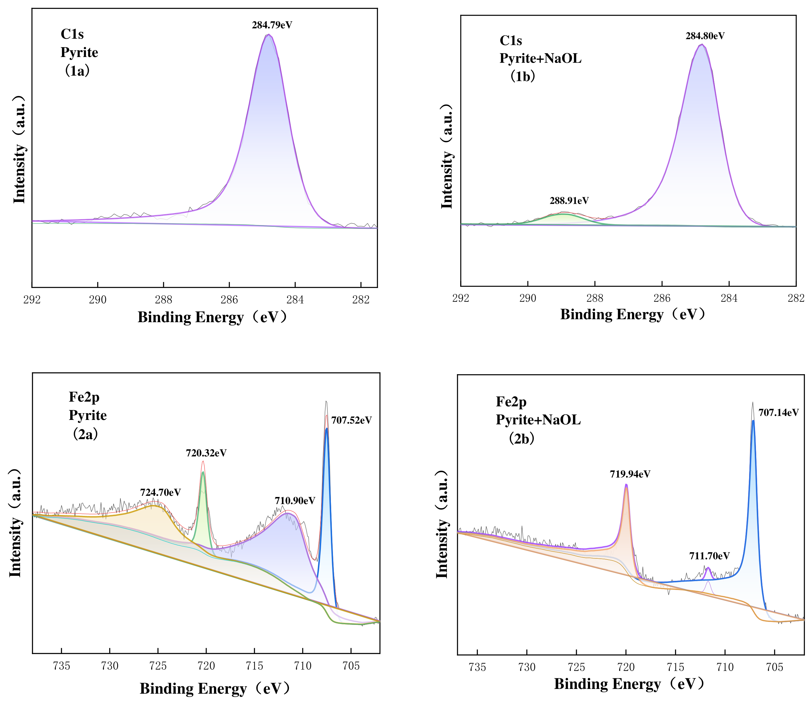
C1s, Fn2p XPS spectra on pyrite surface untreated (1a,2a), treated with NaOL (1b,2b). The different colored lines and shaded areas represent the deconvoluted component peaks.
Figure 15.
C1s, Fn2p XPS spectra on pyrite surface untreated (1a,2a), treated with NaOL (1b,2b). The different colored lines and shaded areas represent the deconvoluted component peaks.
Figure 16.
SEM image of the phosphate concentrate. The numbered points indicate specific mineral phases identified via EDS point analysis: 1 fluorapatite.
Figure 16.
SEM image of the phosphate concentrate. The numbered points indicate specific mineral phases identified via EDS point analysis: 1 fluorapatite.
Figure 17.
SEM image of the de-magnesium tailings. The numbered points indicate specific mineral phases identified via EDS point analysis: 1 dolomite.
Figure 17.
SEM image of the de-magnesium tailings. The numbered points indicate specific mineral phases identified via EDS point analysis: 1 dolomite.
Figure 18.
SEM image of the desilication tailings. The numbered points indicate specific mineral phases identified via EDS point analysis: 1 fluorapatite, 2 quartz.
Figure 18.
SEM image of the desilication tailings. The numbered points indicate specific mineral phases identified via EDS point analysis: 1 fluorapatite, 2 quartz.
Figure 19.
SEM image of the phosphate concentrate. The numbered points indicate specific mineral phases identified via EDS point analysis: 1 pyrite, 2 pyrite, and 3 fluorapatite.
Figure 19.
SEM image of the phosphate concentrate. The numbered points indicate specific mineral phases identified via EDS point analysis: 1 pyrite, 2 pyrite, and 3 fluorapatite.
Table 1.
SEM-EDS elemental composition (wt.%) of the run-of-mine ore, corresponding to the point analyses in
Figure 3.
Table 1.
SEM-EDS elemental composition (wt.%) of the run-of-mine ore, corresponding to the point analyses in
Figure 3.
| Number | Element | Content (%) |
|---|
| 1 | S | 11.38 |
| Fe | 30.31 |
| Zn | 14.81 |
| Pb | 43.51 |
| 2 | Fe | 19.69 |
| S | 2.94 |
| Pb | 64.74 |
| Zn | 12.62 |
| 3 | Fe | 47.43 |
| S | 3.50 |
| Zn | 30.15 |
| Pb | 18.92 |
Table 2.
Mass yield distribution of artificially mixed minerals using different collectors.
Table 2.
Mass yield distribution of artificially mixed minerals using different collectors.
| Mixed Mineral System | Collector | Dosage (mol/L) | pH | Yield of Froth Product (%) | Yield of Sink Product (%) |
|---|
| Mixture I (with Dolomite) | NaOL | 1 × 10⁻³ | 5.0 | 93.23 | 6.77 |
| Mixture II (with Quartz) | DTAB | 1 × 10⁻⁴ | 5.0 | 54.91 | 45.09 |
Table 3.
Metallurgical performance of the anionic reverse flotation stage for dolomite rejection and the partitioning of Pb and Zn.
Table 3.
Metallurgical performance of the anionic reverse flotation stage for dolomite rejection and the partitioning of Pb and Zn.
| Products | Yield | Assay | Lead Content | Zinc Content |
|---|
| (%) | MgO | Fe2O3 | Al2O3 | SiO2 | CaO | P2O5 | (ppm) | (ppm) |
|---|
| Concentrate | 79.9 | 1.14 | 2.43 | 4.29 | 17.49 | 37.73 | 26.23 | 40.7 | 13.3 |
| Tailing | 13.2 | 7.77 | 2.14 | 3.93 | 14.37 | 31.02 | 11.66 | 48.6 | 37.2 |
| Middling | 6.9 | 11.81 | 2.08 | 2.68 | 14.47 | 31.86 | 12.67 | 49.7 | 37.2 |
| Feed | 100 | 2.75 | 2.37 | 4.13 | 16.87 | 36.44 | 23.38 | 42.36 | 18.1 |
Table 4.
Metallurgical performance of the cationic reverse flotation stage for desilication and the partitioning of Pb and Zn.
Table 4.
Metallurgical performance of the cationic reverse flotation stage for desilication and the partitioning of Pb and Zn.
| Products | Yield | Assay | Lead Content | Zinc Content |
|---|
| (%) | MgO | Fe2O3 | Al2O3 | SiO2 | CaO | P2O5 | (ppm) | (ppm) |
|---|
| Concentrate | 69.5 | 0.96 | 1.88 | 2.17 | 10.33 | 45.02 | 31.47 | 32.8 | 8.5 |
| Tailing | 30.5 | 7.40 | 2.38 | 4.17 | 26.14 | 29.40 | 19.85 | 44.9 | 16.1 |
| Feed | 100.0 | 2.93 | 2.03 | 2.78 | 15.16 | 40.25 | 27.92 | 41.2 | 13.78 |
Table 5.
Lead and Zinc Content in Different Particle Size Fractions.
Table 5.
Lead and Zinc Content in Different Particle Size Fractions.
| Size | Yield (%) | Lead Content (ppm) | Zinc Content (ppm) |
|---|
| −150 + 74 μm | 18.65 | 28 | 21.3 |
| −74 + 50 μm | 26.91 | 29.2 | 22.9 |
| −50 + 38 μm | 14.26 | 29 | 26.2 |
| −38 μm | 38.21 | 42.8 | 33.6 |
Table 6.
SEM-EDS elemental composition (wt.%) of the fluorapatite, corresponding to the point analyses in
Figure 16.
Table 6.
SEM-EDS elemental composition (wt.%) of the fluorapatite, corresponding to the point analyses in
Figure 16.
| Number | Element | Content (%) |
|---|
| 1 | O | 59.182 |
| F | 4.565 |
| P | 11.277 |
| Ca | 24.708 |
| Zn | 0.221 |
| Pb | 0.047 |
Table 7.
SEM-EDS elemental composition (wt.%) of the dolomite, corresponding to the point analyses in
Figure 17.
Table 7.
SEM-EDS elemental composition (wt.%) of the dolomite, corresponding to the point analyses in
Figure 17.
| Number | Element | Content (%) |
|---|
| 1 | C | 27.427 |
| O | 55.353 |
| Mg | 7.549 |
| Ca | 9.610 |
| Zn | 0.055 |
| Pb | 0.017 |
Table 8.
SEM-EDS elemental composition (wt.%) of the fluorapatite and quartz, corresponding to the point analyses in
Figure 18.
Table 8.
SEM-EDS elemental composition (wt.%) of the fluorapatite and quartz, corresponding to the point analyses in
Figure 18.
| Number | Element | Content (%) |
|---|
| 1 | O | 65.102 |
| F | 6.276 |
| P | 9.223 |
| Ca | 19.141 |
| Zn | 0.172 |
| Pb | 0.087 |
| 2 | O | 44.061 |
| Mg | 1.137 |
| Al | 24.260 |
| Si | 28.706 |
| Fe | 1.650 |
| Zn | 0.141 |
| Pb | 0.044 |
Table 9.
SEM-EDS elemental composition (wt.%) of the pyrite and fluorapatite, corresponding to the point analyses in
Figure 19.
Table 9.
SEM-EDS elemental composition (wt.%) of the pyrite and fluorapatite, corresponding to the point analyses in
Figure 19.
| Number | Element | Content (%) |
|---|
| 1 | S | 46.83 |
| Fe | 43.72 |
| Zn | 0.04 |
| 2 | Fe | 40.76 |
| S | 38.87 |
| 3 | O | 27.37 |
| Ca | 47.19 |
| Fe | 0.96 |
| F | 1.96 |
| P | 17.19 |
| C | 5.23 |
| Zn | 0.06 |
| Pb | 0.04 |