
Finite Element Simulation of Hot Rolling for Large-Scale AISI 430 Ferritic Stainless-Steel Slabs Using Industrial Rolling Schedules—Part 2: Simulation of the Roughing Stage and Comparison with Experimental Results

 ,
, 
 and
and
Abstract
1. Introduction
2. Materials and Methods
2.1. Experimental Procedure
2.2. Material
2.3. FEM Simulation
2.3.1. Numerical Setup and Assumptions
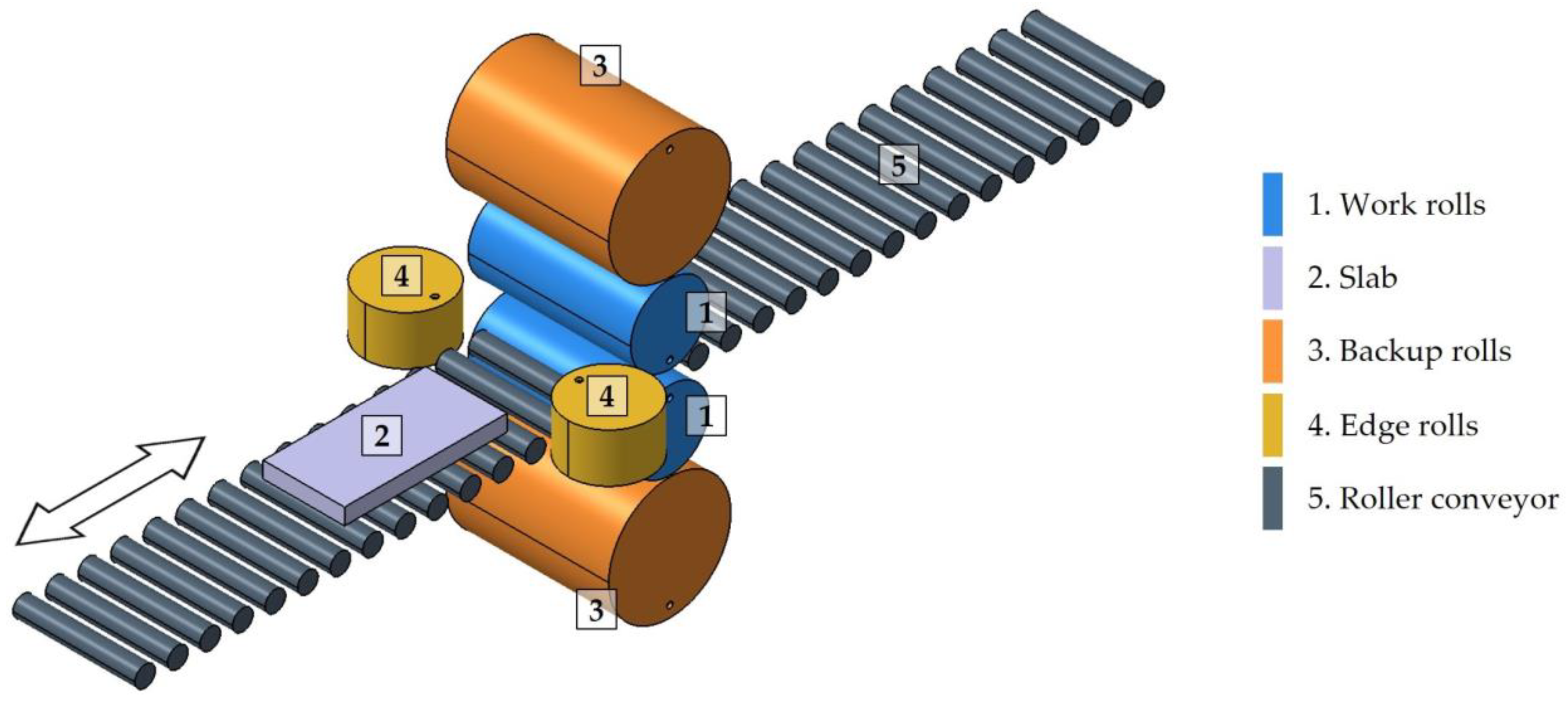
- Both the geometry and the boundary conditions of the studied process are symmetric with respect to the midplane that divides the width of the workpiece into two equal parts. Therefore, only half of the slab was simulated, with a width of 640 mm. This approach allowed the omission of one edge roll and a reduction in the dimensions of the remaining rolls.
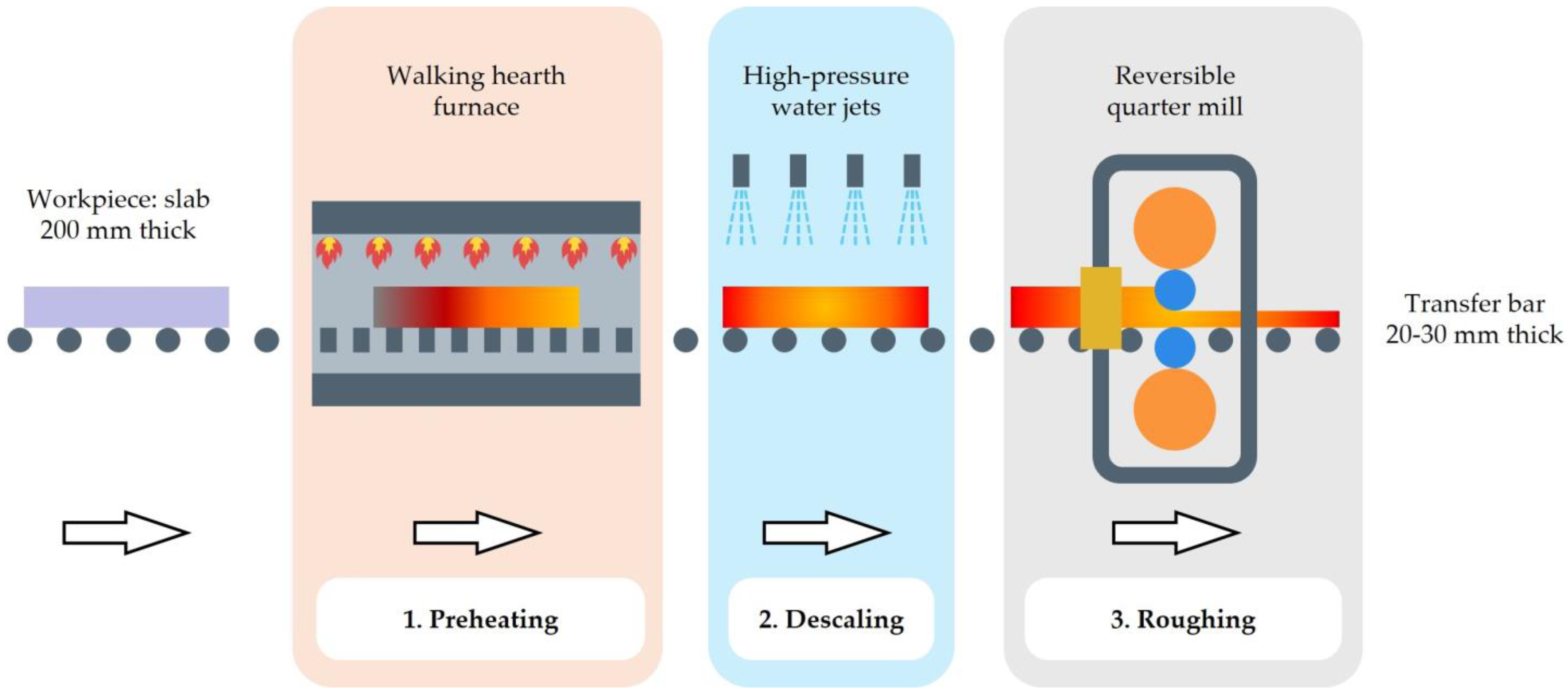
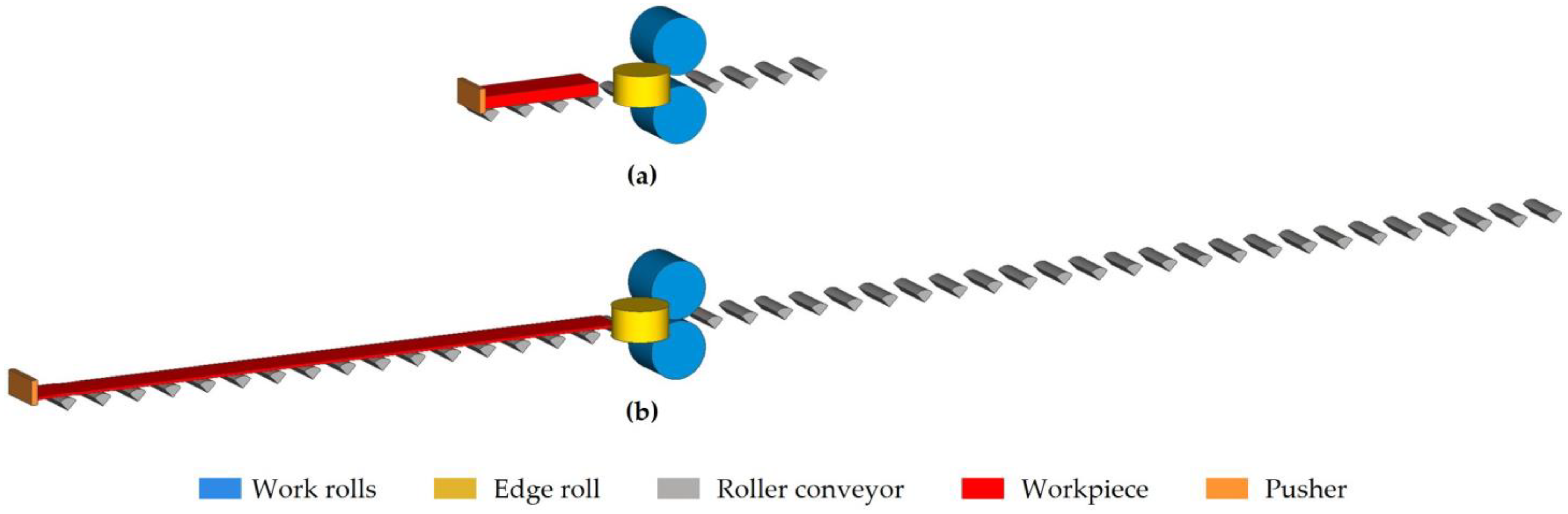
- At the beginning of the rolling process, the slab is moved by the action of a pusher and slides over a roller conveyor composed of roller sections in the form of quarter cylinders. Upon reaching the edge roll and the work rolls, the slab is gripped, and the pusher ceases to operate. From this point onward, the slab advances due to the action of the rolls.
- The friction between the roller conveyor and the slab, as well as between the pusher and the slab, is zero.
- Oxide scale formation is not considered in the simulation.
- The sides of the workpiece are free surfaces, and the external tractions on the slab surface are zero.
2.3.2. Model Geometry and Mesh Characteristics
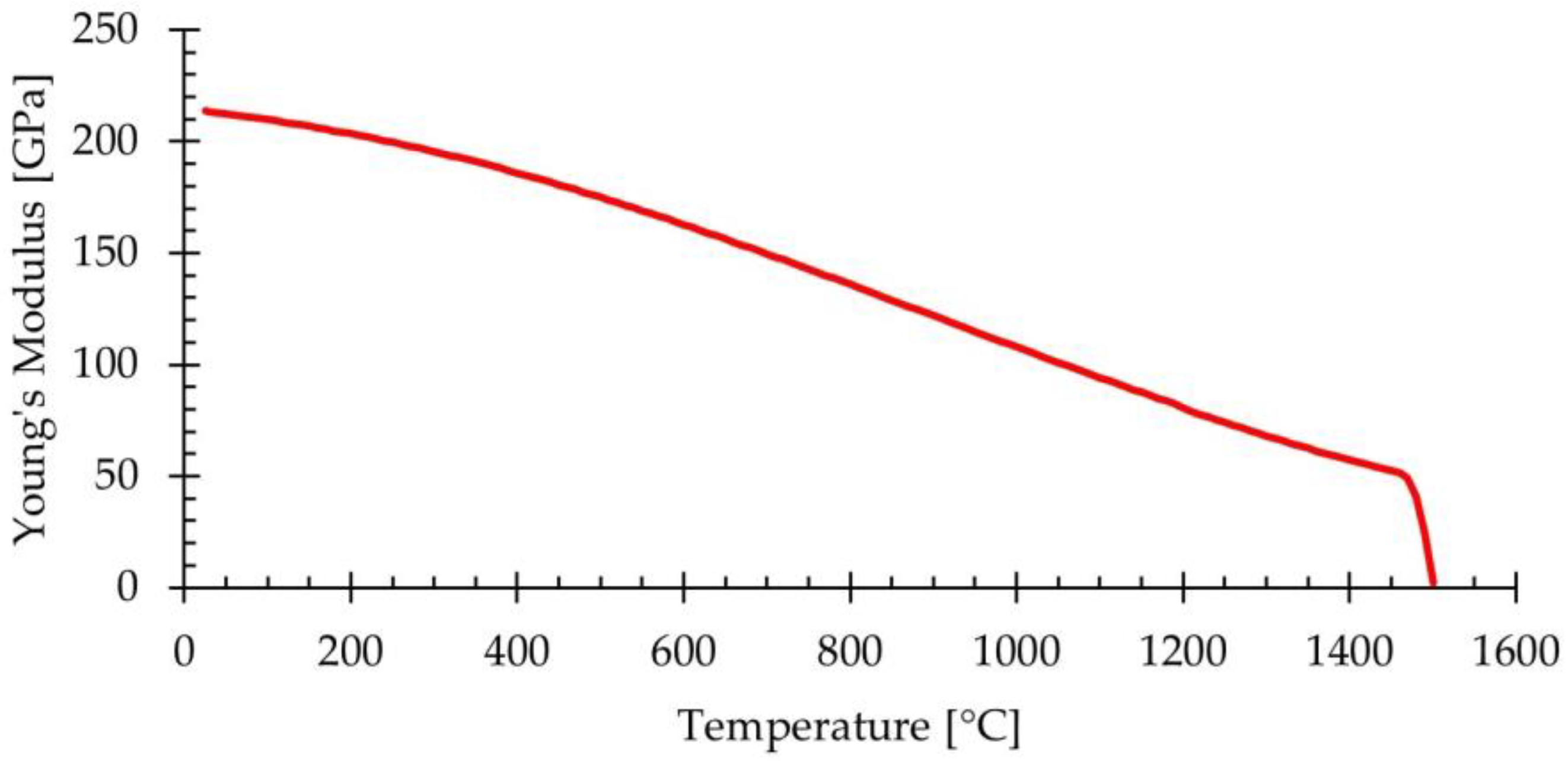
2.3.3. Material Model and Properties
2.3.4. Process Parameters
3. Results and Discussion
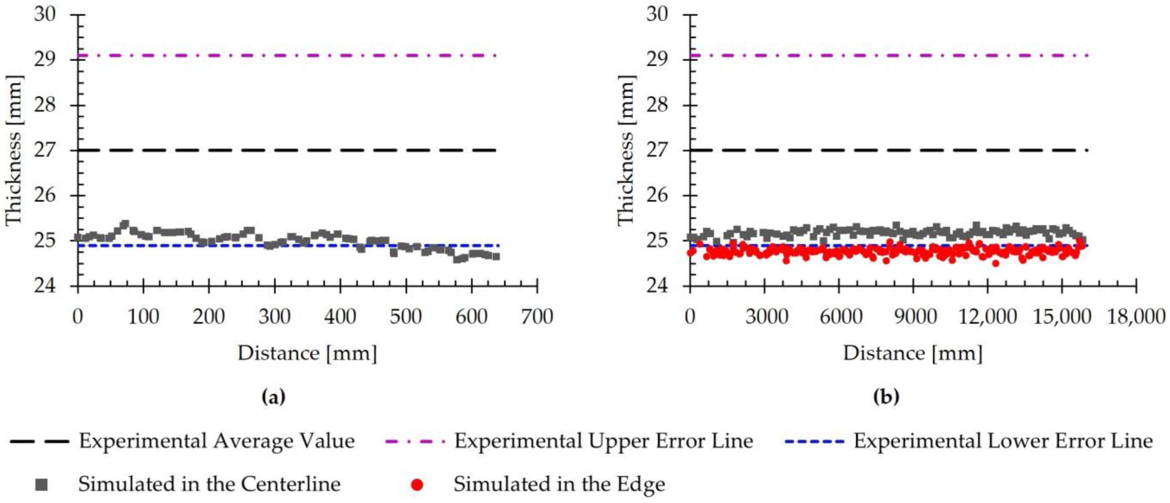
3.1. Thickness
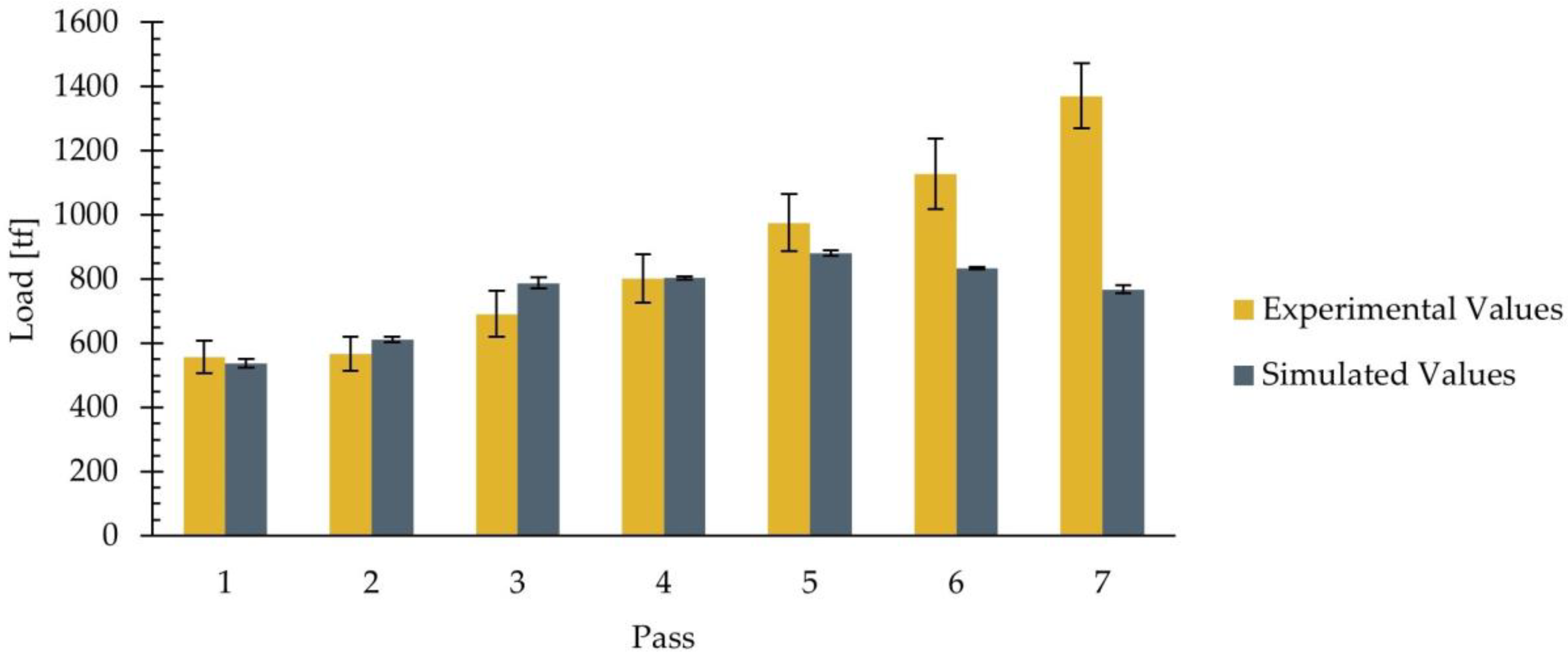
3.2. Rolling Load
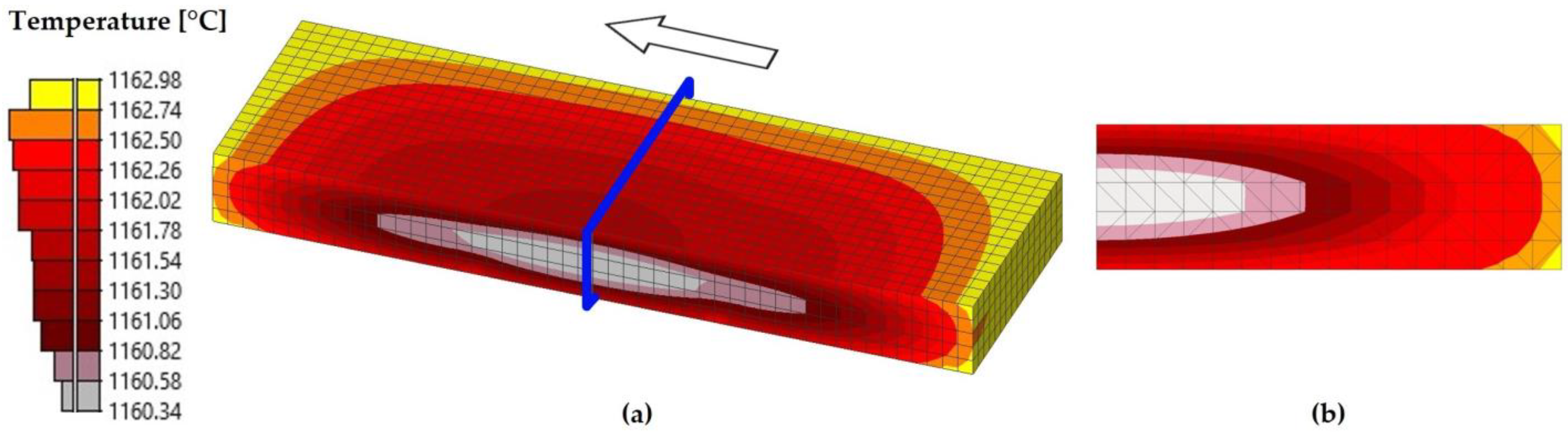
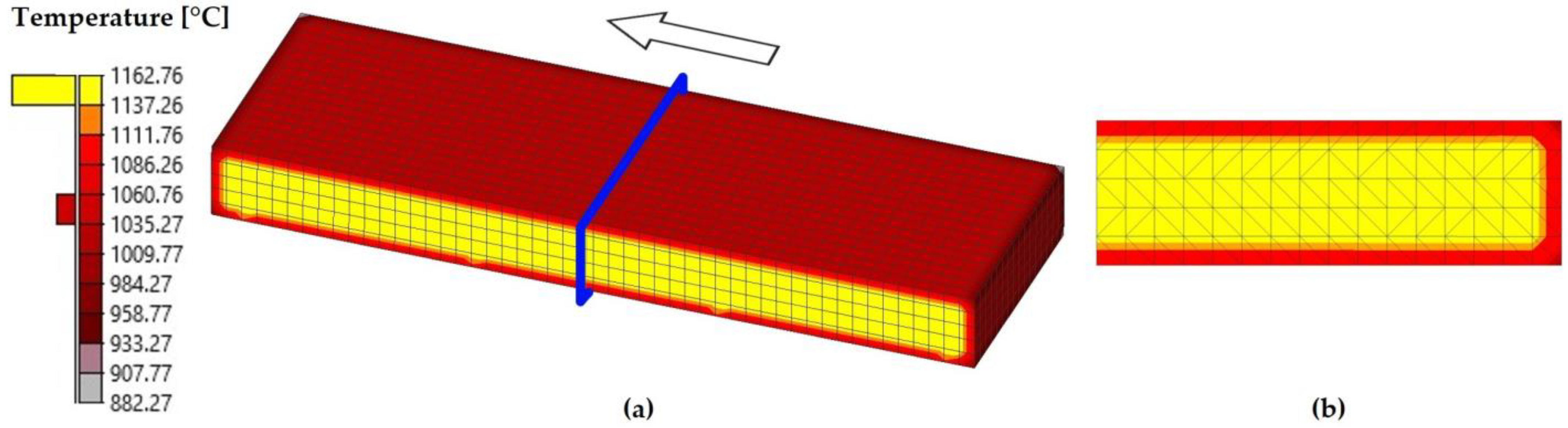
3.3. Temperature
3.4. Effective Plastic Strain
3.5. Equivalent Stress
4. Outlook
5. Summary and Conclusions
- The finite element numerical model used enabled the simulation of the preheating and descaling, and the seven passes of the roughing stage in the industrial rolling schedule of large-scale AISI 430 ferritic stainless-steel slabs. Through the simulation, a transfer bar with an approximate length of 16,100 mm, a width of 1280 mm, and an average thickness of 25.1 mm was obtained.
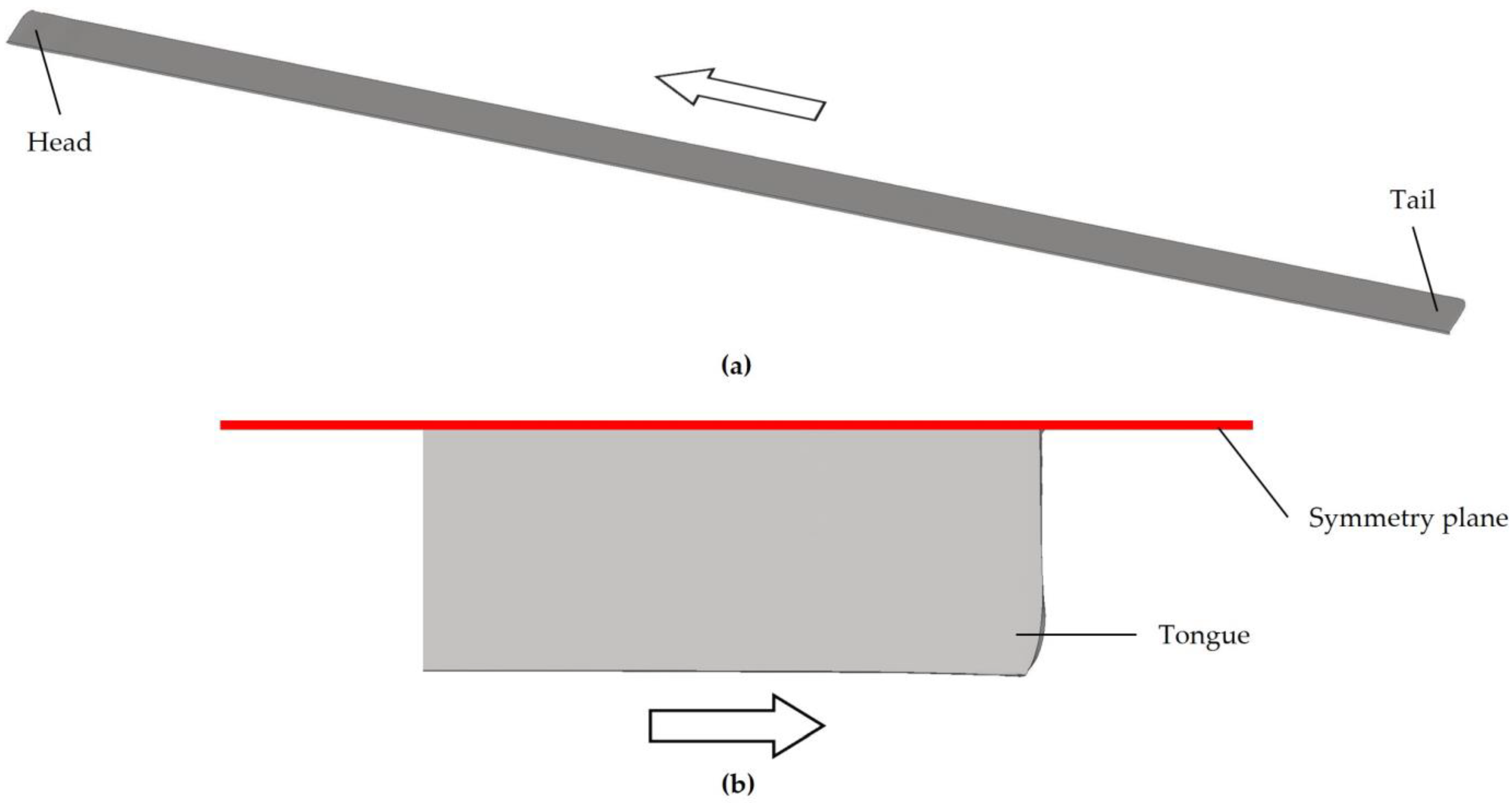
- The transfer bar obtained from the simulation exhibited rounding at both the head and tail. This phenomenon, known as tongues, is common in the hot rolling of flat products as a result of non-uniform deformation in these regions.
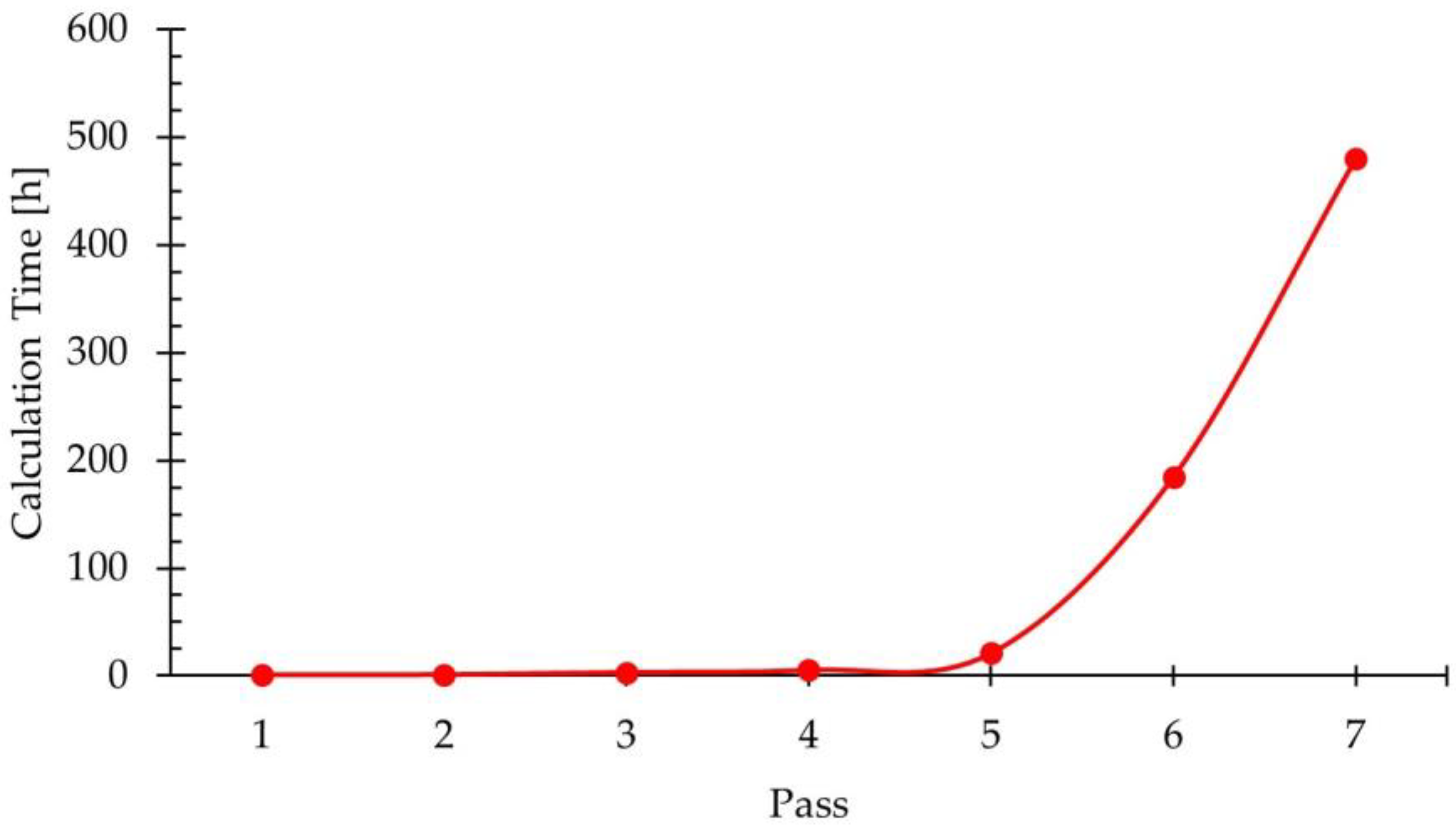
- It was observed that the calculation time required to complete the simulation of each pass increased exponentially. This was due to the reduction in the thickness of the rolled product, which led to a decrease in element size in order to maintain five layers of elements in the thickness direction. Consequently, the number of elements comprising the mesh of the workpiece increased, directly impacting the calculation time.
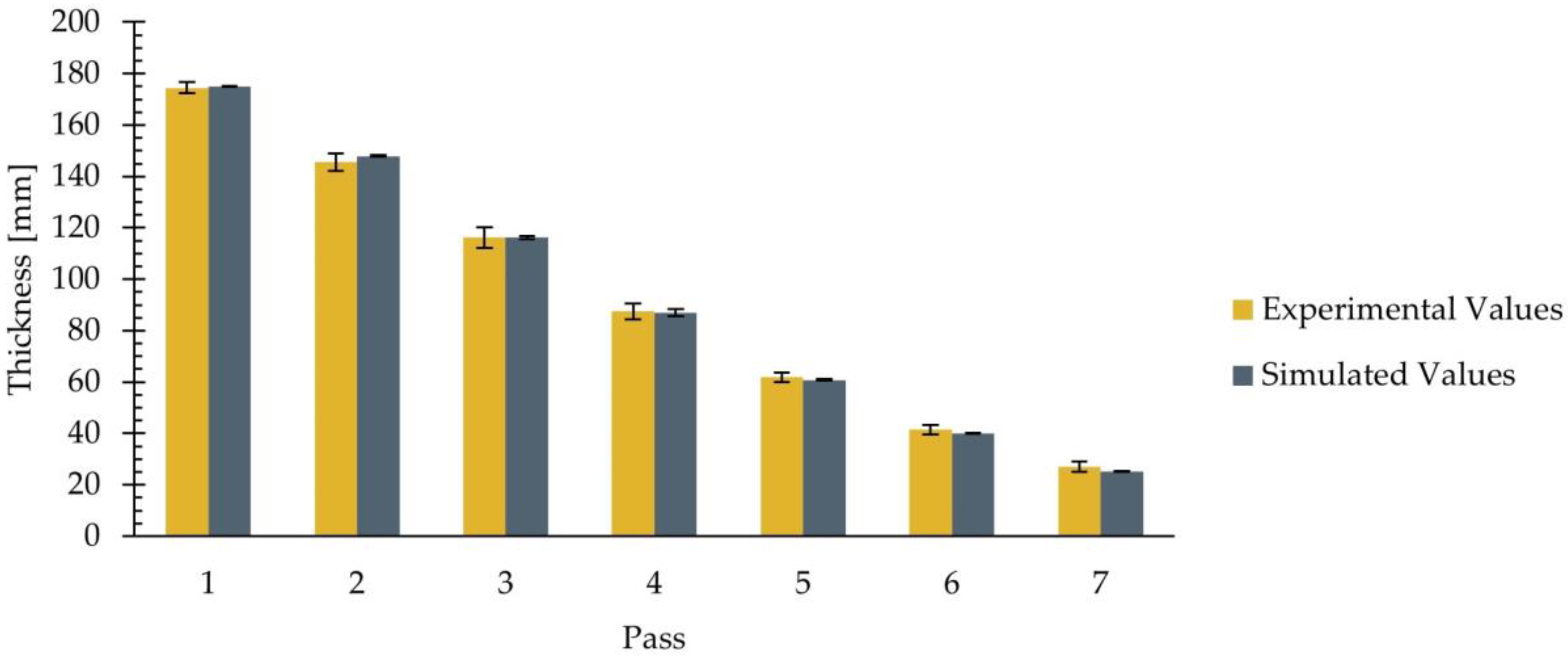
- The average values of the simulated workpiece thickness were in agreement with the experimental data in each of the studied passes. When analyzing the thickness distribution in the final pass, the simulation allowed detecting slight variations in thickness between the centerline and edges of the transfer bar.
- Regarding the rolling load, the results indicate that the employed model allowed estimating the load with an error below 3.5% in the first five passes. In contrast, the relative error in passes six and seven was 18.2% and 39.5%, respectively. After reviewing the available literature, the authors determined that the observed differences could be attributed to the existence of slight differences between the stainless steel used experimentally and that used as a model. Therefore, it will be necessary to further study these differences with the final objective of refining the constitutive equation used in the simulations.
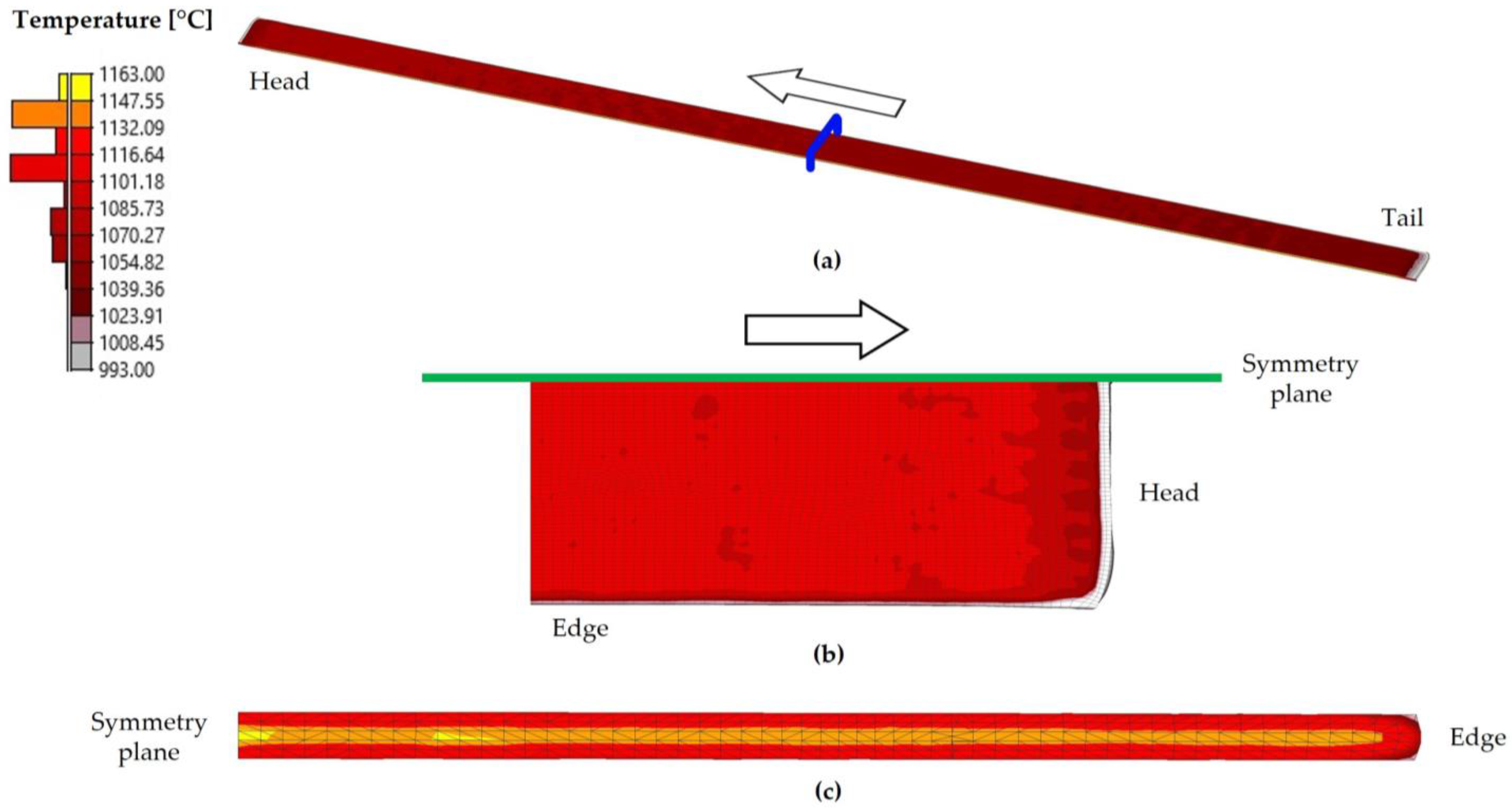
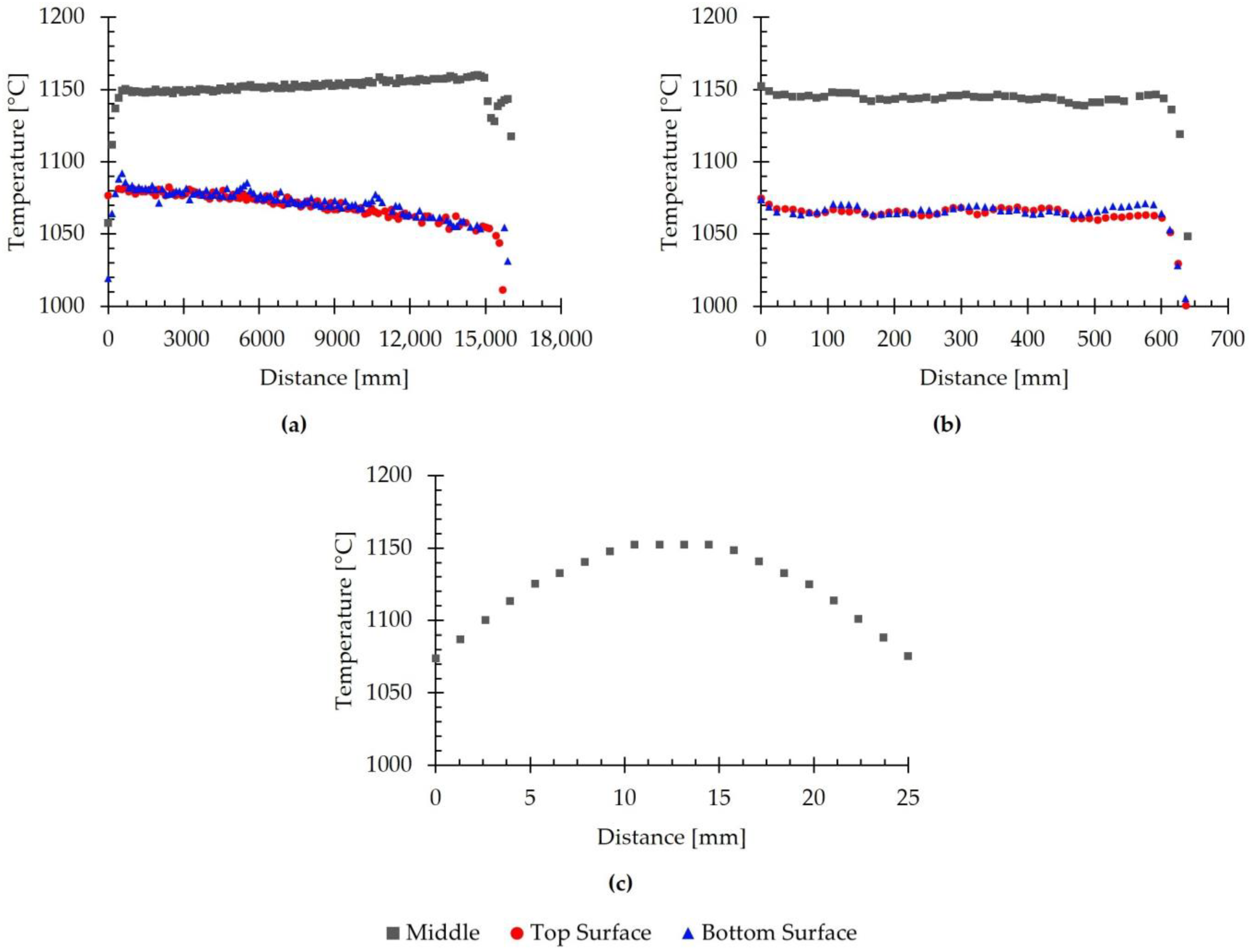
- The surface temperature results at the end of the seventh pass resemble the experimental data, with a difference of 0.6%. When analyzing the temperature distribution, gradients were observed near the surface of the workpiece. The highest temperatures were found in the interior of the material, whereas the lowest temperatures were located on the surfaces.
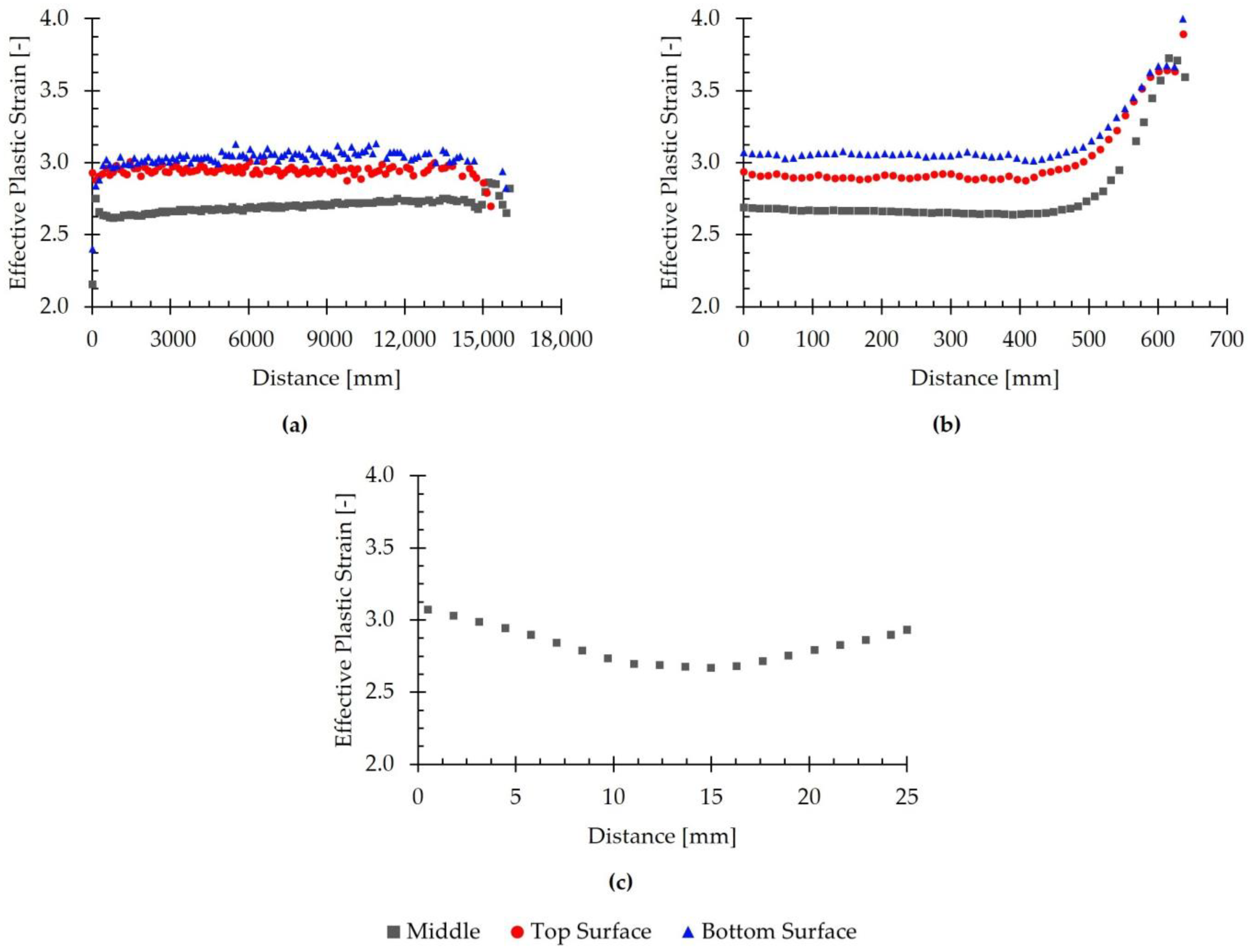
- A non-uniform effective plastic strain distribution was obtained, with higher values at the free surfaces and lower values in the core. According to the literature, this gradient results from restricted material flow in the central region and increased surface deformation due to friction-induced heating.
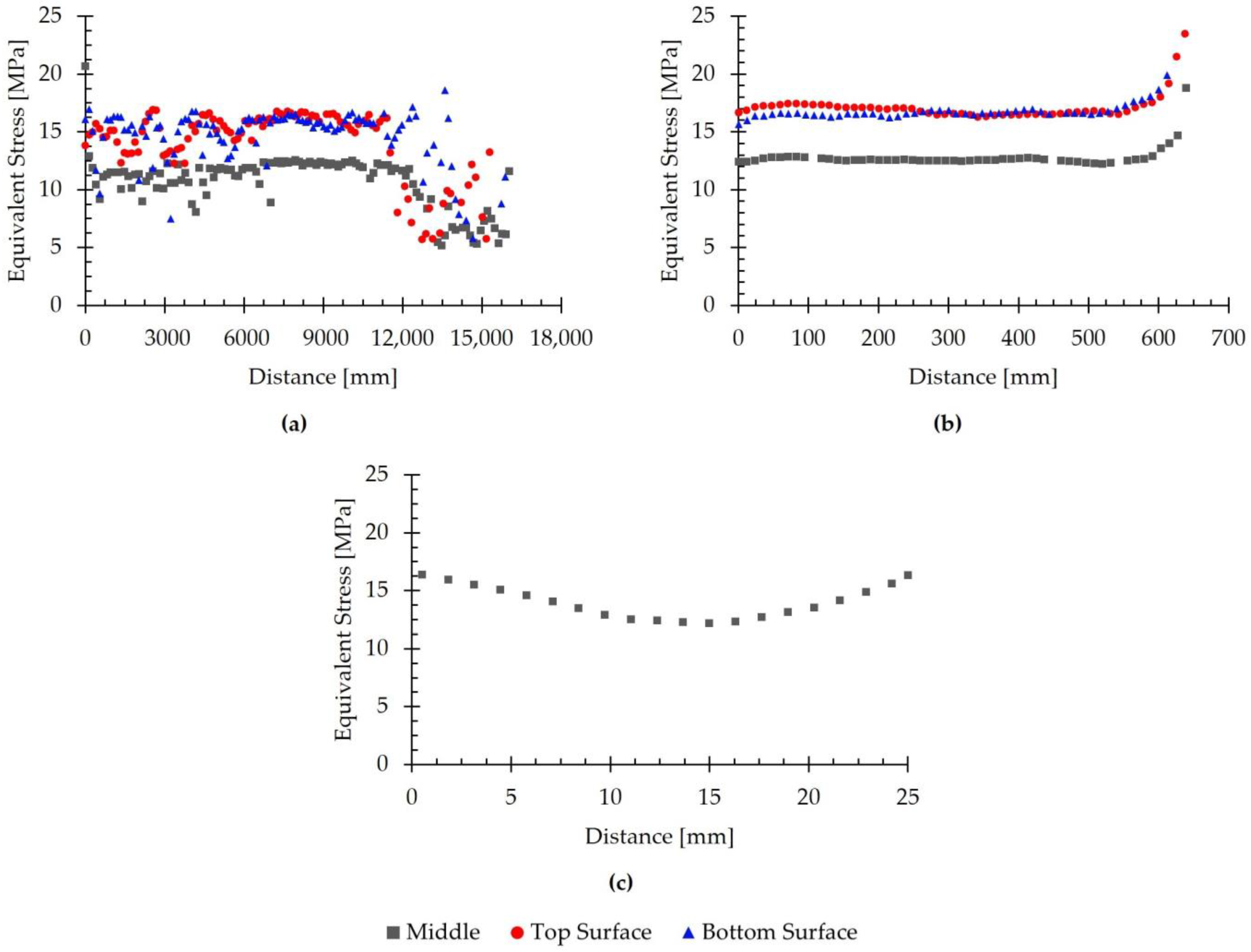
- The simulated equivalent stress exhibited a distribution similar to that of the equivalent plastic strain, with higher values on the free surfaces of the material and lower values in the interior.
- Temperature, plastic deformation, and equivalent stress differences were observed at the edges of the rolled product. These differences could lead to anomalous behaviors in these regions of the material, and their existence will be confirmed in future work through experimental studies.
Author Contributions
Funding
Institutional Review Board Statement
Informed Consent Statement
Data Availability Statement
Acknowledgments
Conflicts of Interest
References
- Hanoglu, U.; Šarler, B. Multi-Pass Hot-Rolling Simulation Using a Meshless Method. Comput. Struct. 2018, 194, 1–14. [Google Scholar] [CrossRef]
- Panjkovic, V. Friction and the Hot Rolling of Steel; CRC Press: Boca Raton, FL, USA, 2014. [Google Scholar]
- Lenards, J.G.; Pietrzyk, M.; Ceser, L. Mathematical and Physical Simulation of the Properties of Hot Rolled Products; Elsevier: Oxford, UK, 1999. [Google Scholar]
- Zienkiewicz, O.C.; Taylor, R. The Finite Element Method. Solid Mechanics; Butterworth-Heinermann: Woburn, UK, 2000; Volume 2. [Google Scholar]
- Hsiang, S.-H.; Lin, S.-L. Application of 3D FEM-Slab Method to Shape Rolling. Int. J. Mech. Sci. 2001, 43, 1155–1177. [Google Scholar] [CrossRef]
- Montmitonnet, P.; Gratacos, P.; Ducloux, R. Application of Anisotropic Viscoplastic Behaviour in 3D Finite-Element Simulations of Hot Rolling. J. Mater. Process Technol. 1996, 58, 201–211. [Google Scholar] [CrossRef]
- Kim, H.J.; Kim, T.H.; Hwang, S.M. A New Free Surface Scheme for Analysis of Plastic Deformation in Shape Rolling. J. Mater. Process Technol. 2000, 104, 81–93. [Google Scholar] [CrossRef]
- Milenin, A.A.; Dyja, H.; Mróz, S. Simulation of Metal Forming during Multi-Pass Rolling of Shape Bars. J. Mater. Process Technol. 2004, 153–154, 108–114. [Google Scholar] [CrossRef]
- Aretz, H.; Luce, R.; Wolske, M.; Kopp, R.; Goerdeler, M.; Marx, V.; Pomana, G.; Gottstein, G. Integration of Physically Based Models into FEM and Application in Simulation of Metal Forming Processes. Model. Simul. Mater. Sci. Eng. 2020, 8, 881–891. [Google Scholar] [CrossRef]
- Liu, G.R. Meshfree Methods: Moving Beyond the Finite Element Method; CRC Press: Boca Raton, FL, USA, 2010. [Google Scholar]
- Chenot, J.L.; Bellet, M. Numerical Modelling of Material Deformation Processes; Hartley, P., Pillinger, I., Sturgess, C., Eds.; Springer: Berlin/Heidelberg, Germany, 1992. [Google Scholar]
- Glowacki, M. The Mathematical Modelling of Thermo-Mechanical Processing of Steel during Multi-Pass Shape Rolling. J. Mater. Process Technol. 2005, 168, 336–343. [Google Scholar] [CrossRef]
- Ojeda-López, A.; Botana-Galvín, M.; Collado-García, I.; González-Rovira, L.; Botana, F.J. Finite Element Simulation of Hot Rolling for Large-Scale AISI 430 Ferritic Stainless-Steel Slabs Using Industrial Rolling Schedules-Part 1: Set-Up, Optimization, and Validation of Numerical Model. Materials 2025, 18, 383. [Google Scholar] [CrossRef]
- Zhang, H.; Wang, B.; Lin, L.; Feng, P.; Zhou, J.; Shen, J. Numerical Analysis and Experimental Trial of Axial Feed Skew Rolling for Forming Bars. Arch. Civ. Mech. Eng. 2022, 22, 17. [Google Scholar] [CrossRef]
- Wang, F.; Ning, L.; Zhu, Q.; Lin, J.; Dean, T.A. An Investigation of Descaling Spray on Microstructural Evolution in Hot Rolling. Int. J. Adv. Manuf. Technol. 2008, 38, 38–47. [Google Scholar] [CrossRef]
- Phaniraj, M.P.; Behera, B.B.; Lahiri, A.K. Thermo-Mechanical Modeling of Two Phase Rolling and Microstructure Evolution in the Hot Strip Mill: Part I. Prediction of Rolling Loads and Finish Rolling Temperature. J. Mater. Process Technol. 2005, 170, 323–335. [Google Scholar] [CrossRef]
- Faini, F.; Attanasio, A.; Ceretti, E. Experimental and FE Analysis of Void Closure in Hot Rolling of Stainless Steel. J. Mater. Process Technol. 2018, 259, 235–242. [Google Scholar] [CrossRef]
- Rout, M.; Pal, S.K.; Singh, S.B. Finite Element Simulation of a Cross Rolling Process. J. Manuf. Process 2016, 24, 283–292. [Google Scholar] [CrossRef]
- Fletcher, J.D.; Beynon, J.H. Heat Transfer Conditions in Roll Gap in Hot Strip Rolling. Ironmak. Steelmak. 1996, 23, 52–57. [Google Scholar]
- Pourabdollah, P.; Serajzadeh, S. An Upper-Bound Finite Element Solution for Rolling of Stainless Steel 304L under Warm and Hot Deformation Conditions. Multidiscip. Model. Mater. Struct. 2016, 12, 514–533. [Google Scholar] [CrossRef]
- Kohring, F.C. Waterwall Water-Cooling Systems. Iron Steel Eng. 1985, 62, 30–36. [Google Scholar]
- Zhou, L.H.; Bi, H.Y.; Sui, F.L.; Du, W.; Fang, X.S. Influence of Finish Rolling Temperature on Microstructure and Properties of Hot-Rolled SUS436L Stainless Steel. J. Mater. Eng. Perform. 2023, 32, 8441–8451. [Google Scholar] [CrossRef]
- Mukhopadhyay, A.; Howard, I.C.; Sellars, C.M. Development and Validation of a Finite Element Model for Hot Rolling Using ABAQUS/STANDARD. Mater. Sci. Technol. 2004, 20, 1123–1133. [Google Scholar] [CrossRef]
- Sadiq, T.O.; Fadara, T.G.; Aiyedun, P.O.; Idris, J. Numerical Estimation of Rolling Load and Torque for Hot Flat Rolling of Hcss316 at Low Strain Rates Based on Mean Temperature. Int. J. Eng. Res. Afr. 2016, 26, 11–29. [Google Scholar] [CrossRef]
- Mancini, S.; Langellotto, L.; Di Nunzio, P.E.; Zitelli, C.; Di Schino, A. Defect Reduction and Quality Optimization by Modeling Plastic Deformation and Metallurgical Evolution in Ferritic Stainless Steels. Metals 2020, 10, 186. [Google Scholar] [CrossRef]
- Pourabdollah, P.; Serajzadeh, S. A Study on Deformation Behavior of 304L Stainless Steel during and after Plate Rolling at Elevated Temperatures. J. Mater. Eng. Perform. 2017, 26, 885–893. [Google Scholar] [CrossRef]
- Soulami, A.; Burkes, D.E.; Joshi, V.V.; Lavender, C.A.; Paxton, D. Finite-Element Model to Predict Roll-Separation Force and Defects during Rolling of U-10Mo Alloys. J. Nucl. Mater. 2017, 494, 182–191. [Google Scholar] [CrossRef]
- Wang, J.; Guo, L.; Wang, C.; Zhao, Y.; Qi, W.; Yun, X. Prediction of Dynamically Recrystallized Microstructure of AZ31 Magnesium Alloys in Hot Rolling Using an Expanded Dislocation Density Model. J. Mater. Eng. Perform. 2023, 32, 2607–2615. [Google Scholar] [CrossRef]
- Chen, W.C.; Samarasekera, I.V.; Kumar, A.; Hawbolt, E.B. Mathematical Modeling of Heat Flow and Deformation during Rough Rolling. Ironmak. Steelmak. 1993, 20, 113–125. [Google Scholar]
- McLaren, A.J.; Sellars, C.M. Modelling Distribution of Microstructure during Hot Rolling of Stainless Steel. Inst. Mater. 1992, 8, 1090–1094. [Google Scholar] [CrossRef]
- Zhang, X.J.; Hodgson, P.D.; Thomson, P.F. The Effect of Through-Thickness Strain Distribution on the Static Recrystallization of Hot Rolled Austenitic Stainless Steel Strip. J. Mater. Process Technol. 1996, 60, 615–619. [Google Scholar] [CrossRef]
- Xiangyu, G.; Wenquan, N.; Wenle, P.; Zhiquan, H.; Tao, W.; Lifeng, M. Deformation Behavior and Bonding Properties of Cu/Al Laminated Composite Plate by Corrugated Cold Roll Bonding. J. Mater. Res. Technol. 2023, 22, 3207–3217. [Google Scholar] [CrossRef]
- Jiang, L.-Y.; Chen, Y.-F.; Liang, J.-L.; Li, Z.-L.; Wang, T.; Ma, L.-F. Modeling of Layer Thickness and Strain for the Two-Layered Metal Clad Plate Rolling with the Different Roll Diameters. J. Mater. Res. Technol. 2024, 28, 3849–3864. [Google Scholar] [CrossRef]
- Sun, P.; Yang, H.; Huang, R.; Zhang, Y.; Zheng, S.; Li, M.; Koppala, S. The Effect of Rolling Temperature on the Microstructure and Properties of Multi Pass Rolled 7A04 Aluminum Alloy. J. Mater. Res. Technol. 2023, 25, 3200–3211. [Google Scholar] [CrossRef]


| Pass | Initial Thickness [mm] | Reduction Ratio [%] | Work-Roll Gap [mm] | Edge-Roll Gap [mm] | Linear Velocity [m·min−1] |
|---|---|---|---|---|---|
| 1 | 200.0 | 12.8 | 175.2 | 1269.0 | 156 |
| 2 | 174.5 | 16.6 | 147.9 | N/A | 180 |
| 3 | 145.6 | 20.2 | 116.2 | 1253.0 | 196 |
| 4 | 116.2 | 24.8 | 87.0 | N/A | 214 |
| 5 | 87.4 | 29.3 | 60.7 | 1253.0 | 270 |
| 6 | 61.8 | 33.0 | 39.9 | N/A | 279 |
| 7 | 41.4 | 34.8 | 24.9 | 1268.0 | 245 |
| Temperature [°C] | Thermal Expansion Coefficient [°C−1] | Thermal Conductivity [W·m−1·K−1] | Specific Heat Capacity [J·g−1·K−1] | Density [kg·m−3] |
|---|---|---|---|---|
| 800 | 13.05·10−6 | 24.83 | 0.73 | 7704 |
| 900 | 13.69·10−6 | 26.62 | 0.70 | 7480 |
| 1000 | 14.24·10−6 | 27.84 | 0.69 | 7440 |
| 1100 | 14.55·10−6 | 28.74 | 0.69 | 7400 |
| 1200 | 13.97·10−6 | 28.91 | 0.69 | 7360 |
| 1250 | N/D | 30.88 | 0.70 | 7310 |
| Part | Diameter [mm] | Length [mm] | Width [mm] | Thickness [mm] | Element Type | Element Size [mm] |
|---|---|---|---|---|---|---|
| Slab | N/A | 2000 | 640 | 200 | Hexahedral | 40 |
| Work roll | 940 | 800 | N/A | N/A | Tetrahedral | 50 |
| Edge roll | 910 | 500 | N/A | N/A | Tetrahedral | 50 |
| Roll of the roller conveyor | 400 | 800 | N/A | N/A | Tetrahedral | 50 |
| Pusher | N/A | 800 | 400 | 100 | Tetrahedral | 50 |
| Pass Number | Experimental [mm] | Simulated [mm] |
|---|---|---|
| 1 | 174.5 ± 2.1 | 175.1 ± 0.2 |
| 2 | 145.6 ± 3.4 | 147.9 ± 0.3 |
| 3 | 116.2 ± 4.1 | 116.2 ± 0.6 |
| 4 | 87.4 ± 3.2 | 86.9 ± 1.3 |
| 5 | 61.8 ± 1.8 | 60.8 ± 0.3 |
| 6 | 41.4 ± 1.9 | 39.9 ± 0.1 |
| 7 | 27.0 ± 2.1 | 25.1 ± 0.2 |
| Pass Number | Experimental [tf] | Simulated [tf] |
|---|---|---|
| 1 | 557 ± 51 | 538 ± 14 |
| 2 | 567 ± 52 | 611 ± 9 |
| 3 | 691 ± 72 | 788 ± 18 |
| 4 | 802 ± 75 | 804 ± 5 |
| 5 | 975 ± 89 | 880 ± 9 |
| 6 | 1128 ± 109 | 834 ± 4 |
| 7 | 1371 ± 101 | 768 ± 12 |
| Stage/Pass Number | Experimental [°C] | Simulated [°C] |
|---|---|---|
| Preheating | N/A | 1162 ± 1 |
| Descaling | N/A | 1062 ± 38 |
| Pass 1 | N/A | 1053 ± 41 |
| Pass 2 | N/A | 1045 ± 43 |
| Pass 3 | N/A | 1034 ± 42 |
| Pass 4 | N/A | 1029 ± 40 |
| Pass 5 | N/A | 1028 ± 35 |
| Pass 6 | N/A | 1035 ± 29 |
| Pass 7 | 1048 ± 11 | 1065 ± 19 |
Disclaimer/Publisher’s Note: The statements, opinions and data contained in all publications are solely those of the individual author(s) and contributor(s) and not of MDPI and/or the editor(s). MDPI and/or the editor(s) disclaim responsibility for any injury to people or property resulting from any ideas, methods, instructions or products referred to in the content. |
© 2025 by the authors. Licensee MDPI, Basel, Switzerland. This article is an open access article distributed under the terms and conditions of the Creative Commons Attribution (CC BY) license (https://creativecommons.org/licenses/by/4.0/).
Share and Cite
Ojeda-López, A.; Botana-Galvín, M.; Almagro Bello, J.F.; González-Rovira, L.; Botana, F.J. Finite Element Simulation of Hot Rolling for Large-Scale AISI 430 Ferritic Stainless-Steel Slabs Using Industrial Rolling Schedules—Part 2: Simulation of the Roughing Stage and Comparison with Experimental Results. Materials 2025, 18, 1298. https://doi.org/10.3390/ma18061298
Ojeda-López A, Botana-Galvín M, Almagro Bello JF, González-Rovira L, Botana FJ. Finite Element Simulation of Hot Rolling for Large-Scale AISI 430 Ferritic Stainless-Steel Slabs Using Industrial Rolling Schedules—Part 2: Simulation of the Roughing Stage and Comparison with Experimental Results. Materials. 2025; 18(6):1298. https://doi.org/10.3390/ma18061298
Chicago/Turabian StyleOjeda-López, Adrián, Marta Botana-Galvín, Juan F. Almagro Bello, Leandro González-Rovira, and Francisco Javier Botana. 2025. "Finite Element Simulation of Hot Rolling for Large-Scale AISI 430 Ferritic Stainless-Steel Slabs Using Industrial Rolling Schedules—Part 2: Simulation of the Roughing Stage and Comparison with Experimental Results" Materials 18, no. 6: 1298. https://doi.org/10.3390/ma18061298
APA StyleOjeda-López, A., Botana-Galvín, M., Almagro Bello, J. F., González-Rovira, L., & Botana, F. J. (2025). Finite Element Simulation of Hot Rolling for Large-Scale AISI 430 Ferritic Stainless-Steel Slabs Using Industrial Rolling Schedules—Part 2: Simulation of the Roughing Stage and Comparison with Experimental Results. Materials, 18(6), 1298. https://doi.org/10.3390/ma18061298