
Research on Fatigue Life Prediction Method of Spot-Welded Joints Based on Machine Learning


Abstract
1. Introduction
2. Fatigue Testing of Q&P980 Steel Spot-Welded Joint
2.1. Fatigue Test Scheme
2.1.1. Preparation of Fatigue Specimens
2.1.2. Design of Fatigue Experiments
2.2. Fatigue Test Results
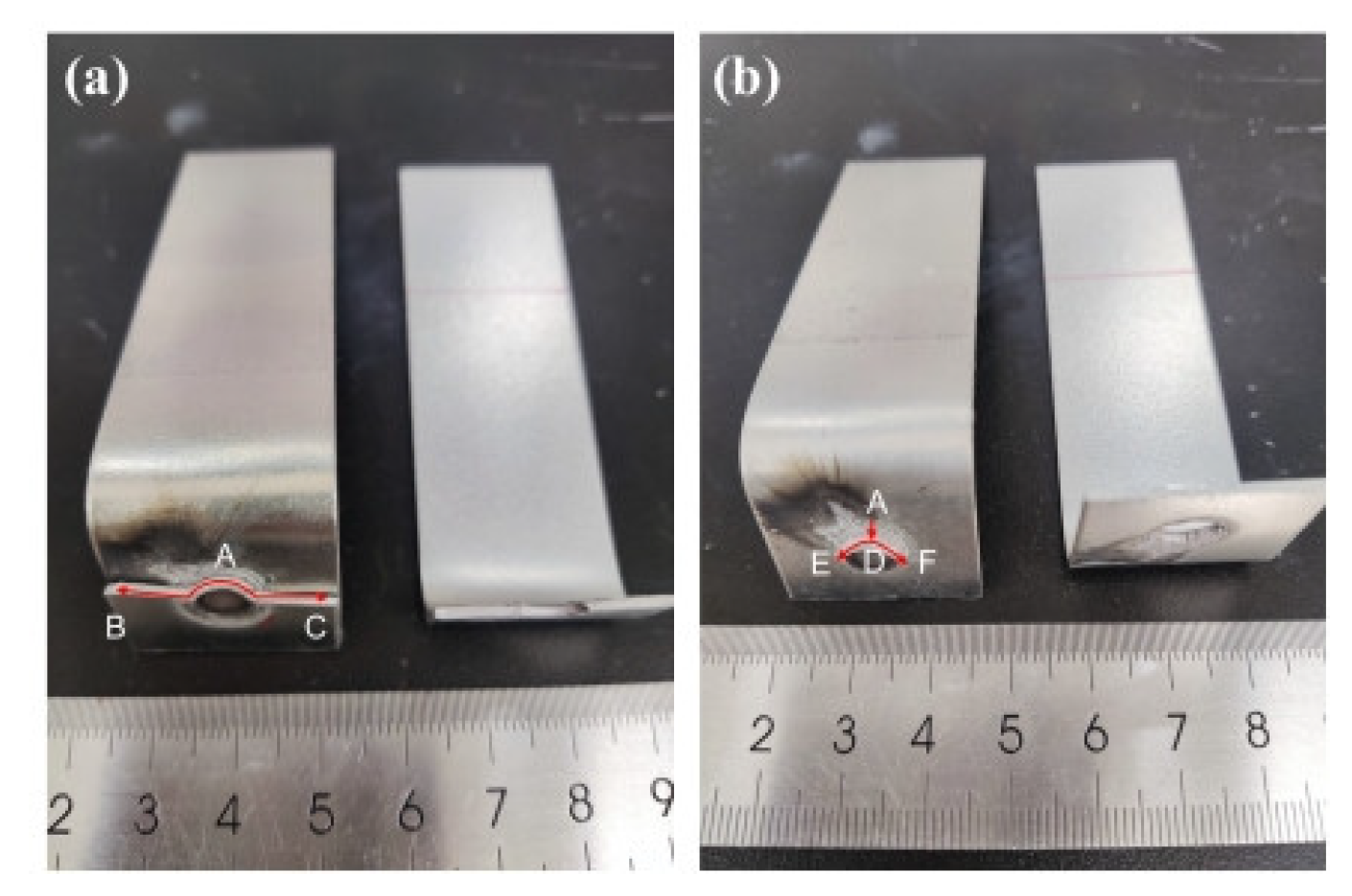
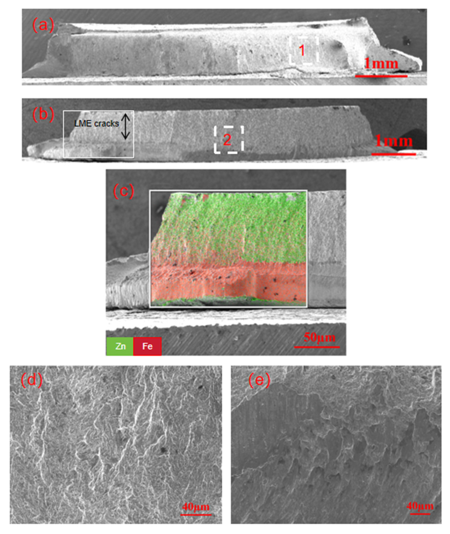
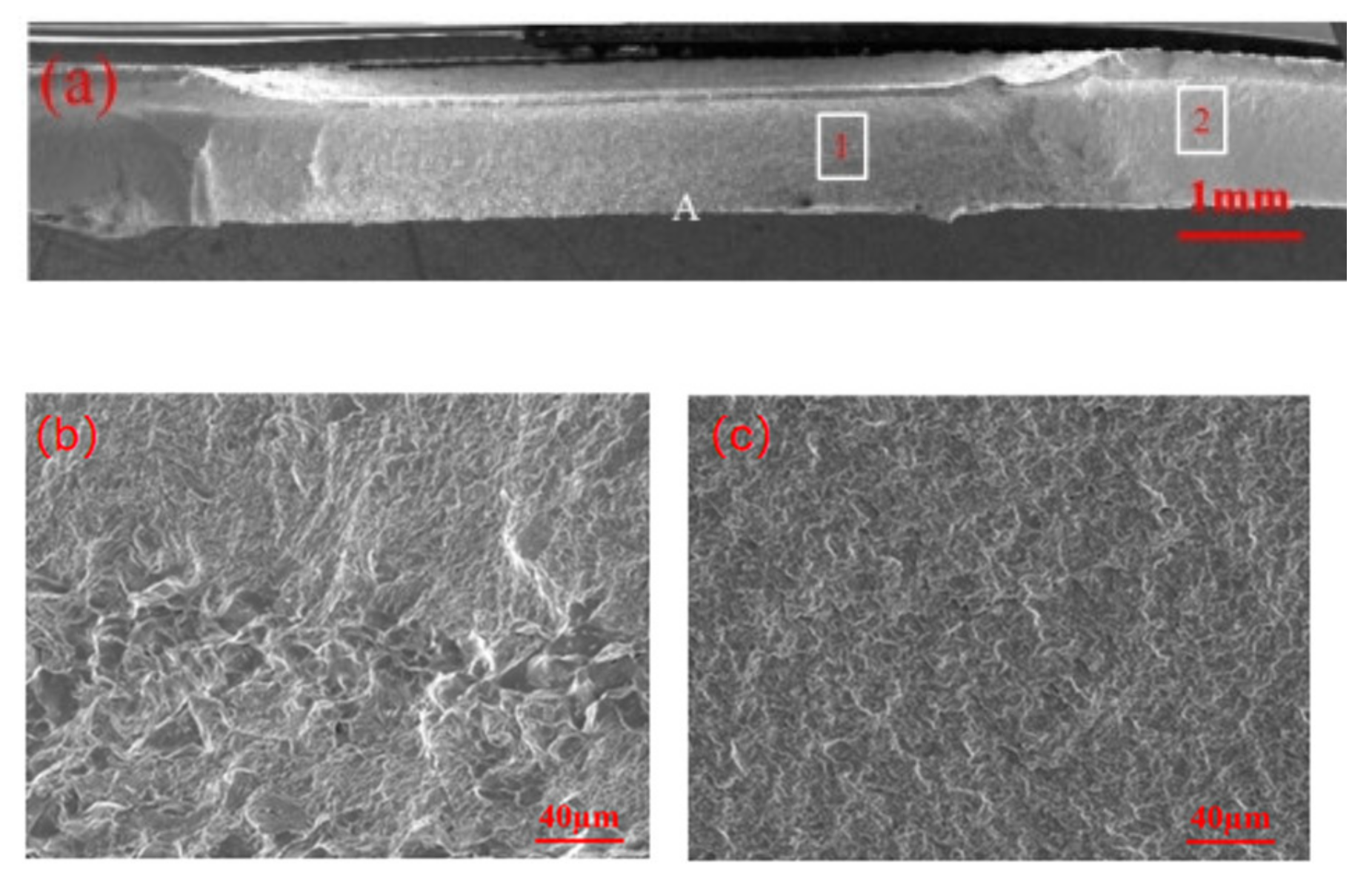
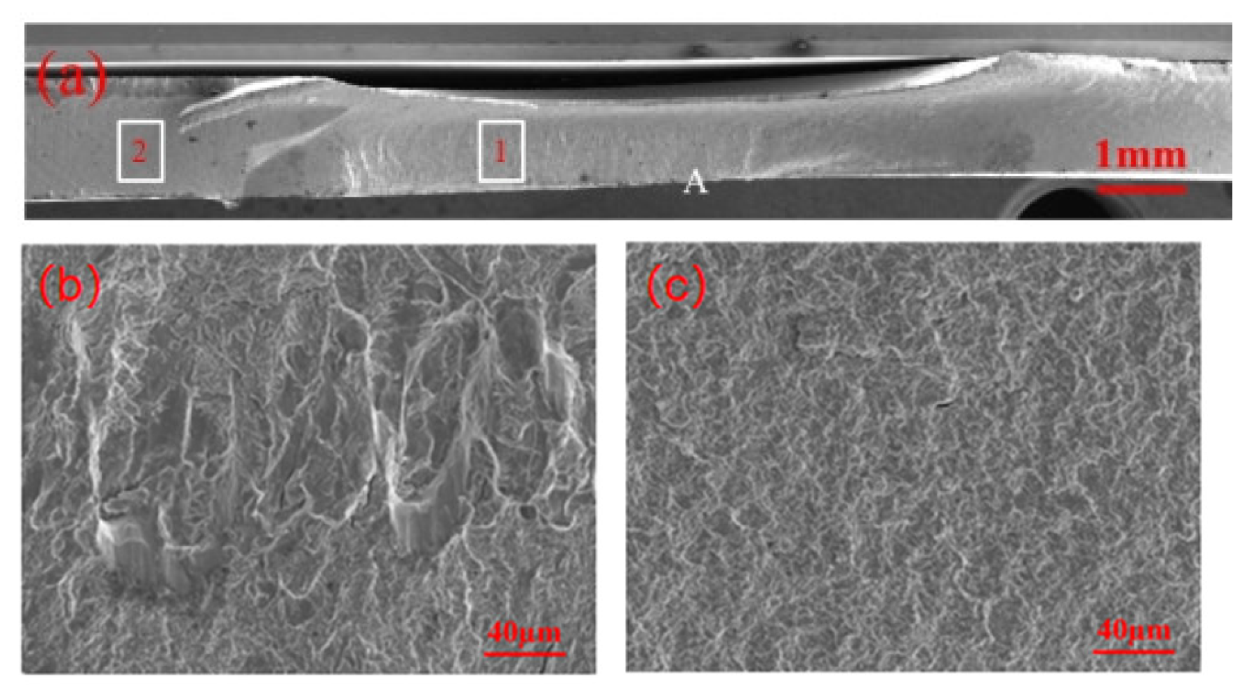
2.3. Fatigue Fracture Analysis
2.3.1. Fatigue Fracture of CP Specimens
2.3.2. Summary of Fatigue Fracture Analysis
3. Fatigue Data Analysis and Preprocessing
3.1. Data Collection
3.2. Data Pre-Processing
3.2.1. Data Normalization
3.2.2. Dataset Division
4. Fatigue Life Prediction Methods for Spot-Welded Joints
4.1. Theoretical Empirical Formulas
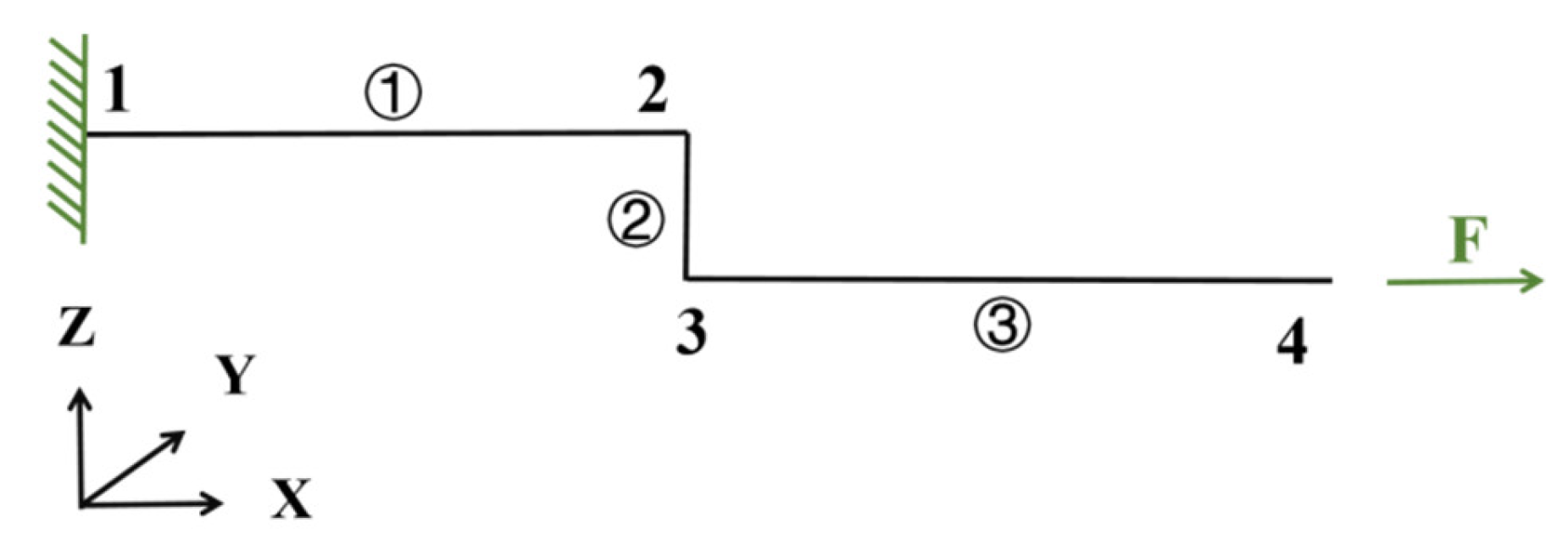
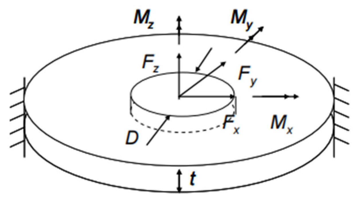
4.1.1. Rupp Structural Stress Method
4.1.2. Rupp-Modified Structural Stress Method
4.1.3. Empirical Formulas for Fitting Curves
4.2. Machine Learning Algorithms
4.2.1. Artificial Neural Network Algorithm
4.2.2. Gaussian Process Regression Algorithm
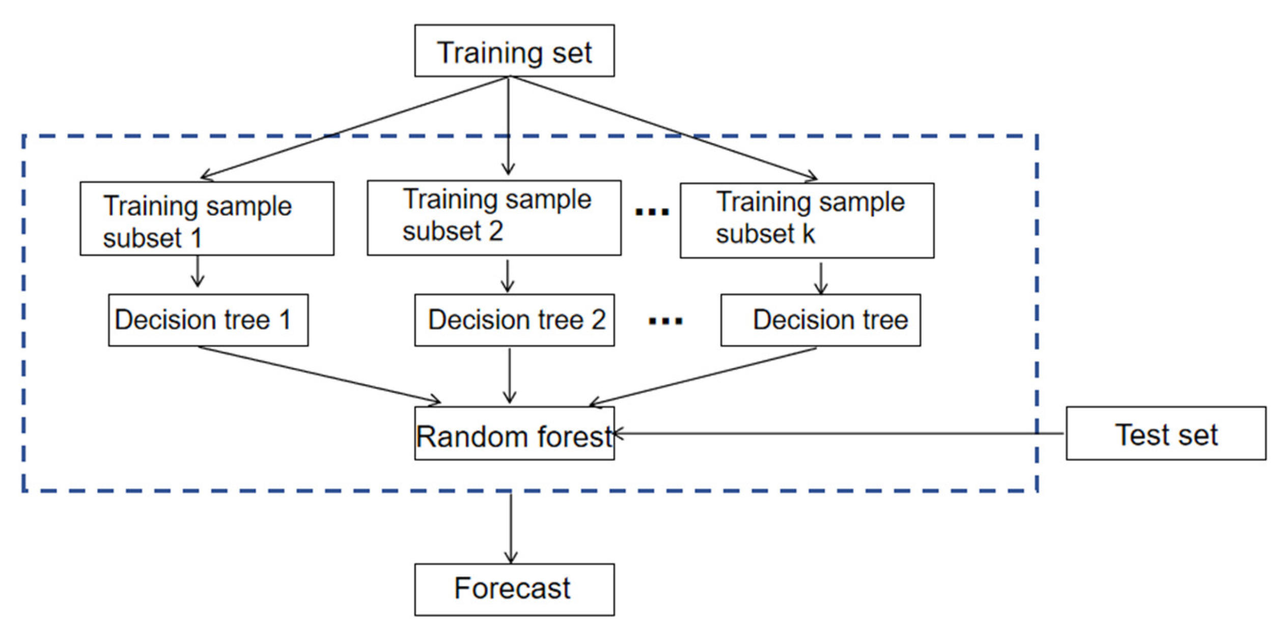
4.2.3. Random Forest Algorithm
4.3. Model Assessment Metrics and Feature Sensitivity Analysis
4.3.1. Model Evaluation Indicators
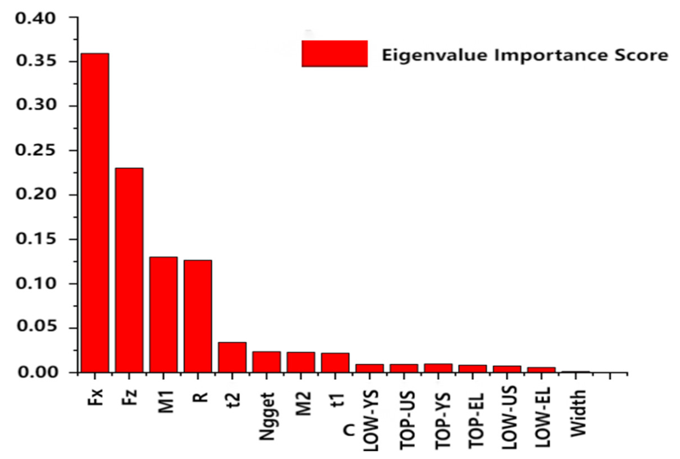
4.3.2. Characterization Sensitivity Analysis
4.4. Analysis of Fatigue Life Prediction Results
4.4.1. Theoretical Empirical Formula Fitting
4.4.2. Analysis of Training Results for the Training Set
4.4.3. Result Discussion
5. Summary
Author Contributions
Funding
Institutional Review Board Statement
Informed Consent Statement
Data Availability Statement
Conflicts of Interest
References
- Kong, F.P.; Zou, S.J. Fatigue life prediction and maintenance strategies in ship structural design. Ship Mater. Mark. 2024, 32, 36–38. [Google Scholar] [CrossRef]
- Zou, J.; Xiang, H.; Zhan, Z.; Zhuo, W.; Huang, L.; Ji, Y.; Liu, Q. Research on the influence of liquid metal embrittlement cracks on the strength and fatigue life of spot-welded joints of galvanized Q&P980 steel. Materials 2024, 17, 6149. [Google Scholar] [PubMed]
- Rupp, A.; Störzel, K.; Grubisic, V. Computer Aided Dimensioning of Spot-Welded Automotive Structures; SAE Technical Paper; SAE: Warrendale, PA, USA, 1995. [Google Scholar]
- Du, W.C. Microstructure, Mechanical Properties, and Liquid Metal Embrittlement of PHS1500 Galvanized Steel Spot Welded Joints. Master’s Dissertation, Jiangsu University of Science and Technology, Zhenjiang, China, 2021. [Google Scholar]
- Liu, Z.; Zhao, Y.; Wang, X. Fatigue life prediction of welded joints using random forest algorithm. J. Mater. Sci. Technol. 2020, 39, 1021–1029. [Google Scholar]
- Wu, G.; Li, D.; Su, X. Fatigue life prediction of spot welded joints based on artificial neural network. Int. J. Fatigue 2019, 135, 105478. [Google Scholar]
- Xu, M.; Qi, H.Y.; Li, S.L.; Shi, D.Q.; Yang, X.G. Machine-Learning-Based Fatigue Life Prediction Method for Welded Joints. Aeroengine 2025, 51, 96–102. [Google Scholar] [CrossRef]
- Pape, F.; Maiss, O.; Denkena, B.; Poll, G. Enhancement of roller bearing fatigue life by innovative production processes. Ind. Lubr. Tribol. 2019, 71, 1003–1006. [Google Scholar] [CrossRef]
- Zhan, L.; Qin, X.G. Fatigue life prediction of stainless steel car body side wall resistance spot welded joints. J. Jiamusi Univ. (Nat. Sci. Ed.) 2017, 35, 799–802. [Google Scholar]
- Han, X.H.; Liu, S.L.; Zhao, Y.Q. Optimization of fatigue performance of high-stress spot welded joints in car bodies based on nugget diameter. China Railw. Sci. 2013, 34, 84–88. [Google Scholar]
- Long, H.Q. Characteristics of Resistance Spot Welding and Fatigue Crack Propagation of DP590/DC01 Dissimilar Thickness Steel Plates. Ph.D. Dissertation, Chongqing University, Chongqing, China, 2017. [Google Scholar]
- Qian, T. Research on Fatigue Life Simulation Prediction Method of High-Strength Steel Weld Points Based on Mean Stress Intensity Factor. Master’s Dissertation, Hunan University, Changsha, China, 2015. [Google Scholar]
- Wang, R. Deformation of Dissimilar Resistance Spot Welded Joints of Low Carbon Steel and Austenitic Stainless Steel and Its Influence on Mechanical Properties. Master’s Dissertation, Beijing Jiaotong University, Beijing, China, 2022. [Google Scholar]
- Zhang, Z.X. Fatigue Performance of Weld Points of DP980-GMW2 and Q&P980-GMW2 Steel Plates. Master’s Thesis, Liaoning University of Science and Technology, Anshan, China, 2016. [Google Scholar]
- Bonnen, J.J.; Agrawal, H.; Amaya, M.A.; Iyengar, R.M.; Kang, H.T.; Khosrovaneh, A.K.; Link, T.M.; Shih, H.C.; Walp, M.; Yan, B. Fatigue of advanced high strength steel spot-welds. Int. J. Fatigue 2006, 28, 726–744. [Google Scholar]
- Wu, G.; Li, D.; Su, X.; Peng, Y.; Shi, Y.; Huang, L.; Huang, S.; Tang, W. Experiment and modeling on fatigue of the DP780GI spot welded joint. Mater. Sci. Eng. A 2017, 103, 73–85. [Google Scholar] [CrossRef]
- Long, X.; Khanna, S.K. Fatigue properties and failure characterization of spot welded high strength steel sheet. Int. J. Fatigue 2007, 29, 879–886. [Google Scholar] [CrossRef]
- Hu, J.H.; Song, K.; Xiong, L.M. Fatigue life study of weld point defects considering the modified mean equivalent stress intensity factor. China Mech. Eng. 2020, 31, 740–745. [Google Scholar]
- Tang, J.Z.; Zou, D.Q.; Jiang, H.M.; Chen, X.P.; Li, S.H. Experimental study on resistance spot welding process and fatigue performance of Q&P steel lap joints. Hot Work. Technol. 2014, 43, 39–42+6. [Google Scholar]
- Huang, L.; Shi, Y.; Guo, H.; Su, X. Fatigue behavior and life prediction of self-piercing riveted joint. Int. J. Fatigue 2016, 88, 96–110. [Google Scholar] [CrossRef]
- Yang, Y.N.; Wang, R.J.; Yan, K. Prediction of fatigue life of spot welded specimens using structural stress method. Weld. Mach. 2016, 46, 50–53. [Google Scholar]
- Mi, X.X.; Tang, A.T.; Zhu, Y.C.; Kang, L.; Pan, F.S. Advances in the application of machine learning techniques in materials science. Mater. Rep. 2021, 35, 15115–15124. [Google Scholar]
- Wang, H.W.; Ye, B.; Feng, J.; Zhong, X.Y. Review on the application of machine learning in steel materials research. China Mater. Prog. 2023, 42, 806–813. [Google Scholar]
- Cheng, M.; Jiao, L.; Yan, P.; Feng, L.; Qiu, T.; Wang, X.; Zhang, B. Prediction of surface residual stress in end milling with Gaussian process regression. J. Manuf. Sci. Eng. 2021, 178, 109333. [Google Scholar] [CrossRef]


| Overlap Style | Load Frequency/Hz | Load Amplitude/N | Specimen Number | Galvanized Specimen | Non-Galvanized Specimen | ||
|---|---|---|---|---|---|---|---|
| Fatigue Life/cyc | Average Lifespan/cyc | Fatigue Life/cyc | Average Lifespan/cyc | ||||
| TS | 30 | 1800 | 1 | 21,053 | 20,892 | 50,637 | 41,403 |
| 2 | 20,438 | 40,997 | |||||
| 3 | 21,185 | 32,575 | |||||
| CP | 10 | 135 | 1 | 33,858 | 29,486 | 24,895 | 26,916 |
| 2 | 25,503 | 23,149 | |||||
| 3 | 29,096 | 32,705 | |||||
| Feature | Label | Range | |
|---|---|---|---|
| Material Properties | tensile strength | US1, US2 | 306–1355 (Mpa) |
| yield strength | YS1, YS2 | 170–1156 (Mpa) | |
| elongation | EL1, EL2 | 5.1–35 (%) | |
| Plate Size | plate thickness | t1, t2 | 0.8–4 (mm) |
| plate width | Width | 35–50 (mm) | |
| Joint Characterization | nucleus diameter | Nugget | 3.9–13.4 (mm) |
| Loading method | stress ratio | R | −1~0.3 |
| Joint force (calculated value) | X-direction force | Fx | 0–23,837 (N) |
| Z-direction force | Fz | 7.81–1851 (N) | |
| Y-direction moment1 | M1 | 493–25,418 (N·mm) | |
| Y-direction moment2 | M2 | 493–33,541 (N·mm) | |
| fatigue life | fatigue life | Nf | 268–107 (cyc) |
| Arithmetic | Evaluation Indicators | ||
|---|---|---|---|
| R2 | RMSE | MAPE | |
| RF | 0.98 | 0.01 | 0.013 |
| GPR | 0.96 | 0.024 | 0.017 |
| ANN | 0.93 | 0.026 | 0.024 |
| Methodologies | Evaluation Indicators | ||
|---|---|---|---|
| R2 | RMSE | MAPE | |
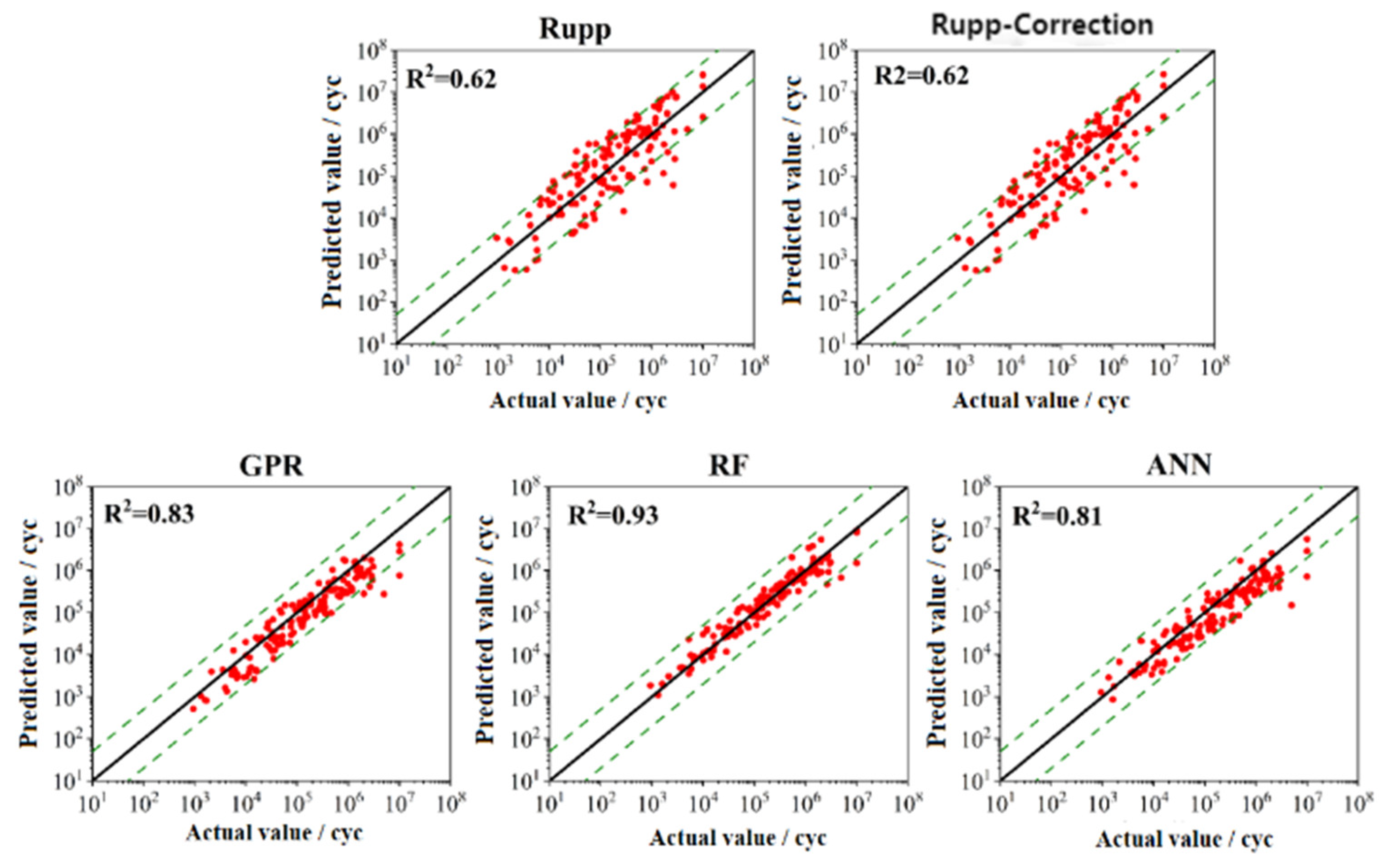
| Rupp | 0.62 | 0.306 | 0.096 |
| Rupp-Amendment | 0.62 | 0.305 | 0.095 |
| RF | 0.93 | 0.056 | 0.033 |
| GPR | 0.83 | 0.139 | 0.061 |
| ANN | 0.81 | 0.152 | 0.06 |
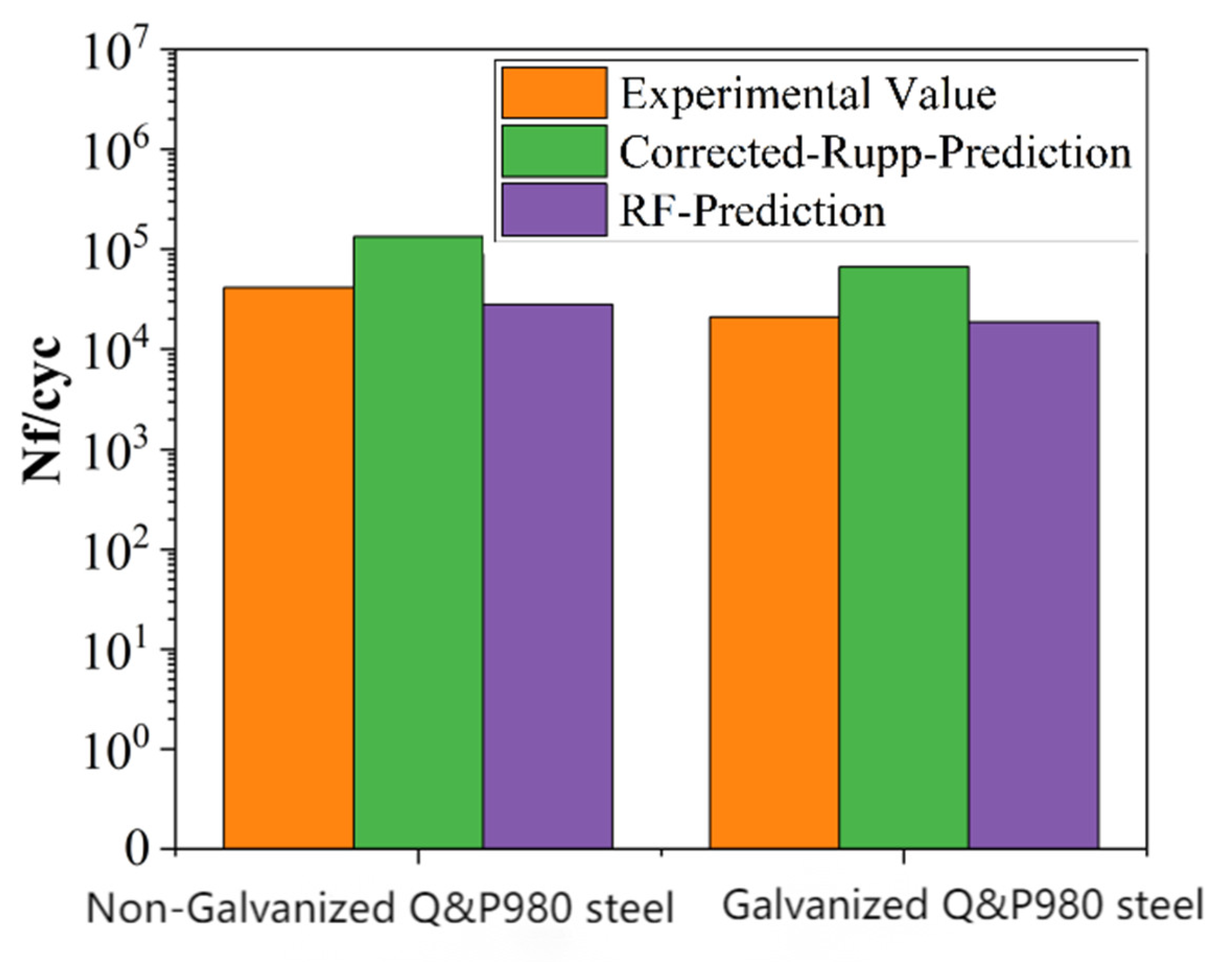
| Specimen Type | Test Result (cyc) | Rupp-Amendment Prediction (cyc) | RF Prediction (cyc) |
|---|---|---|---|
| Galvanized | 20,892 | 66,688 | 18,689 |
| Non-Galvanized | 41,403 | 133,377 | 28,237 |
Disclaimer/Publisher’s Note: The statements, opinions and data contained in all publications are solely those of the individual author(s) and contributor(s) and not of MDPI and/or the editor(s). MDPI and/or the editor(s) disclaim responsibility for any injury to people or property resulting from any ideas, methods, instructions or products referred to in the content. |
© 2025 by the authors. Licensee MDPI, Basel, Switzerland. This article is an open access article distributed under the terms and conditions of the Creative Commons Attribution (CC BY) license (https://creativecommons.org/licenses/by/4.0/).
Share and Cite
Li, S.; Zhan, Z.; Zou, J.; Wang, Z. Research on Fatigue Life Prediction Method of Spot-Welded Joints Based on Machine Learning. Materials 2025, 18, 3542. https://doi.org/10.3390/ma18153542
Li S, Zhan Z, Zou J, Wang Z. Research on Fatigue Life Prediction Method of Spot-Welded Joints Based on Machine Learning. Materials. 2025; 18(15):3542. https://doi.org/10.3390/ma18153542
Chicago/Turabian StyleLi, Shanshan, Zhenfei Zhan, Jie Zou, and Zihan Wang. 2025. "Research on Fatigue Life Prediction Method of Spot-Welded Joints Based on Machine Learning" Materials 18, no. 15: 3542. https://doi.org/10.3390/ma18153542
APA StyleLi, S., Zhan, Z., Zou, J., & Wang, Z. (2025). Research on Fatigue Life Prediction Method of Spot-Welded Joints Based on Machine Learning. Materials, 18(15), 3542. https://doi.org/10.3390/ma18153542