Figure 1.
Geometry of specimens for tensile tests (unit: mm): (a) smooth specimens of the weld seam; (b) smooth specimens of base material; (c) shear specimen; (d) notched specimen with a notch radius of R2: (e) notched specimen with a notch radius of R5; (f) notched specimen with a notch radius of R8.
Figure 2.
Fractured samples in tensile test ( s−1): (a) Usibor1500P; (b) weld seam; (c) Dustibor500.
Figure 2.
Fractured samples in tensile test ( s−1): (a) Usibor1500P; (b) weld seam; (c) Dustibor500.
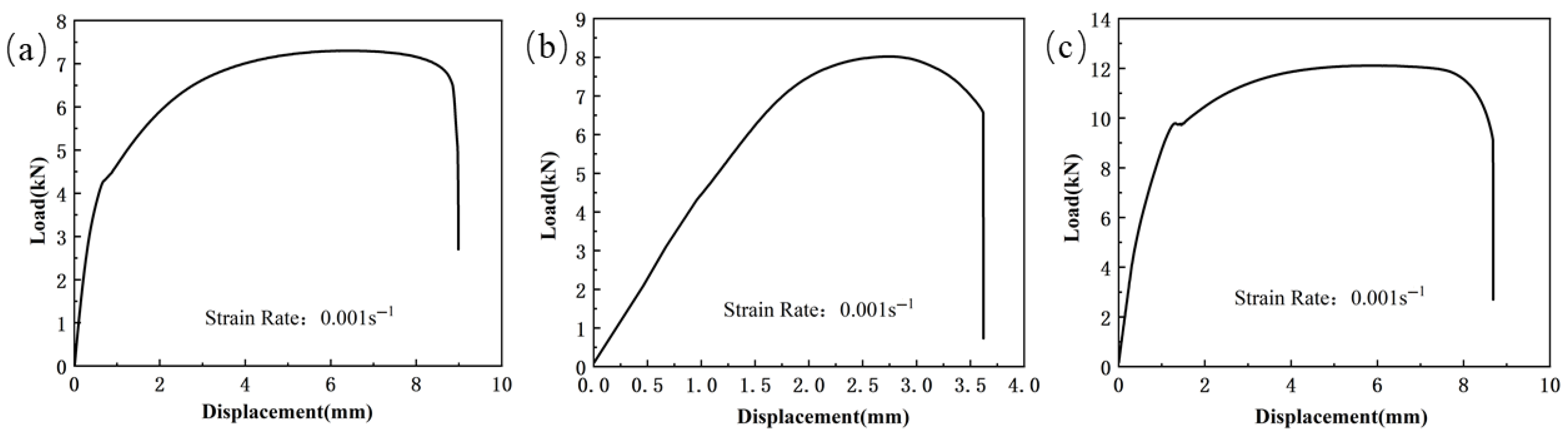
Figure 3.
The load–displacement curve of the shear specimen tensile test for TWBs. ( s−1): (a) Usibor1500P; (b) Weld seam; (c) Dustibor500.
Figure 3.
The load–displacement curve of the shear specimen tensile test for TWBs. ( s−1): (a) Usibor1500P; (b) Weld seam; (c) Dustibor500.
Figure 4.
The load–displacement curve of the smooth specimen tensile test for TWBs ( s−1): (a) Usibor1500P; (b) weld seam; (c)
Dustibor500.
Figure 4.
The load–displacement curve of the smooth specimen tensile test for TWBs ( s−1): (a) Usibor1500P; (b) weld seam; (c)
Dustibor500.
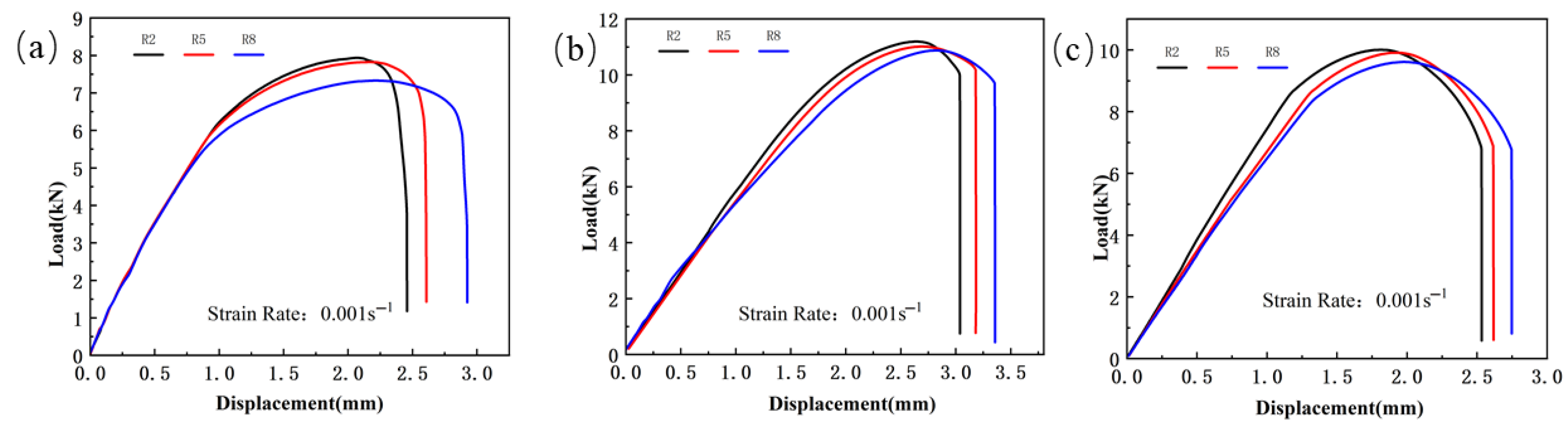
Figure 5.
The load–displacement curve of the notched specimen tensile test for TWBs ( s−1): (a) Usibor1500P; (b) weld seam; (c) Dustibor500.
Figure 5.
The load–displacement curve of the notched specimen tensile test for TWBs ( s−1): (a) Usibor1500P; (b) weld seam; (c) Dustibor500.
Figure 6.
The mesh divisions of various tensile specimens: (a) welded smooth specimen; (b) base material smooth specimen; (c) shear specimen; (d) R2 notched specimens; (e) R5 notched specimen; (f) R8 notched specimen.
Figure 6.
The mesh divisions of various tensile specimens: (a) welded smooth specimen; (b) base material smooth specimen; (c) shear specimen; (d) R2 notched specimens; (e) R5 notched specimen; (f) R8 notched specimen.
Figure 7.
True stress–strain curve during the tensile test of the smooth specimen (20 °C, s−1): (a) Usibor1500P; (b) weld seam; (c) Dustibor500.
Figure 7.
True stress–strain curve during the tensile test of the smooth specimen (20 °C, s−1): (a) Usibor1500P; (b) weld seam; (c) Dustibor500.
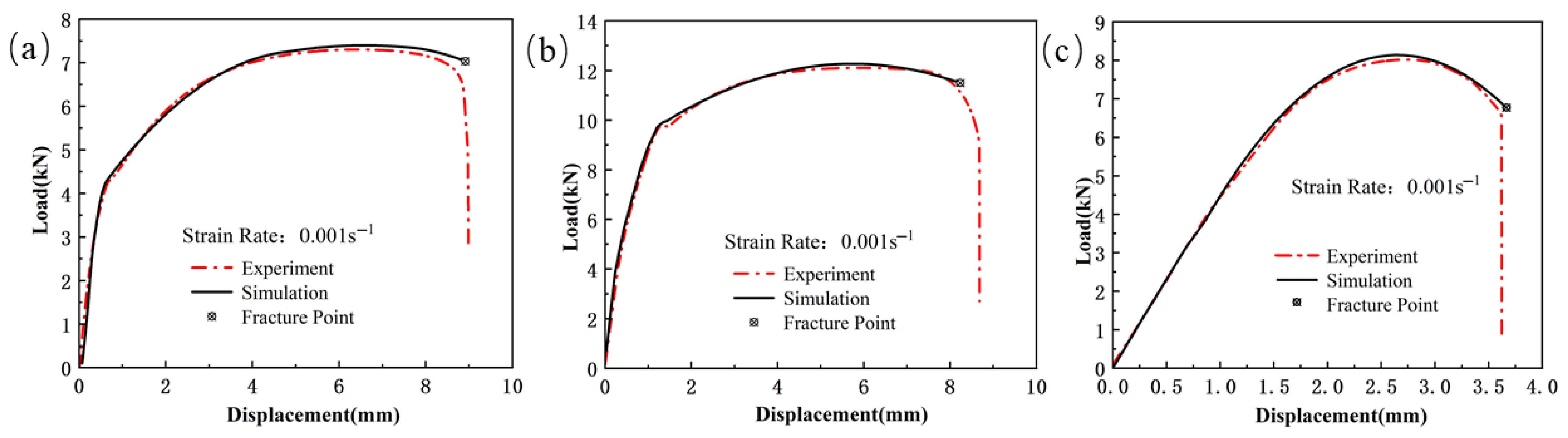
Figure 8.
Comparison of the load–displacement curves between the simulation and the experiment for the shear specimen. ( s−1): (a) Usibor1500P; (b) weld seam; (c) Dustibor500.
Figure 8.
Comparison of the load–displacement curves between the simulation and the experiment for the shear specimen. ( s−1): (a) Usibor1500P; (b) weld seam; (c) Dustibor500.
Figure 9.
Comparison of the load–displacement curves between the simulation and the experiment for the smooth specimen. ( s−1): (a) Usibor1500P; (b) weld seam; (c) Dustibor500.
Figure 9.
Comparison of the load–displacement curves between the simulation and the experiment for the smooth specimen. ( s−1): (a) Usibor1500P; (b) weld seam; (c) Dustibor500.
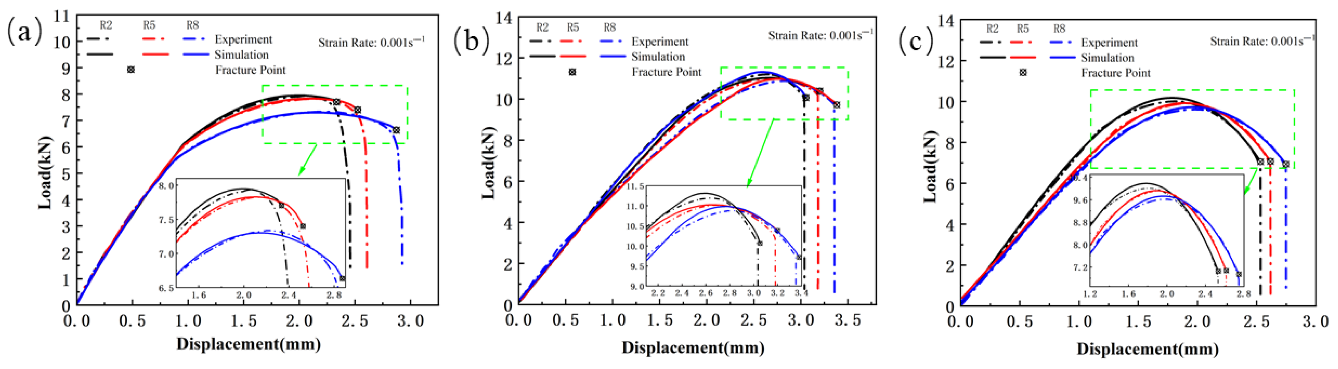
Figure 10.
Comparison of the load–displacement curves between the simulation and the experiment for the notched specimen. ( s−1): (a) Usibor1500P; (b) weld seam; (c) Dustibor500.
Figure 10.
Comparison of the load–displacement curves between the simulation and the experiment for the notched specimen. ( s−1): (a) Usibor1500P; (b) weld seam; (c) Dustibor500.
Figure 11.
Schematic diagram of the specimen’s minimum cross-section.
Figure 11.
Schematic diagram of the specimen’s minimum cross-section.
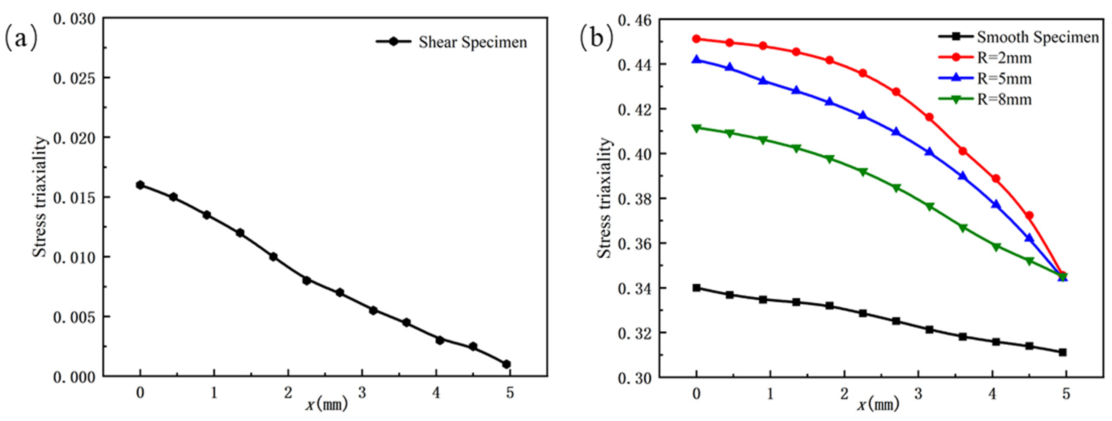
Figure 12.
The distribution of stress triaxiality at the minimum cross-section for each type of specimen: (a) shear specimen; (b) smooth specimen and notched specimens.
Figure 12.
The distribution of stress triaxiality at the minimum cross-section for each type of specimen: (a) shear specimen; (b) smooth specimen and notched specimens.
Figure 13.
The relationship curve between stress triaxiality and PEEQ for each type of specimen ( s−1): (a) Usibor1500P; (b) weld seam; (c) Dustibor500.
Figure 13.
The relationship curve between stress triaxiality and PEEQ for each type of specimen ( s−1): (a) Usibor1500P; (b) weld seam; (c) Dustibor500.
Figure 14.
Distribution of PEEQ and stress triaxiality at the moment of specimen fracture: (a) shear; (b) smooth; (c) R2 notch; (d) R5 notch; (e) R8 notch.
Figure 14.
Distribution of PEEQ and stress triaxiality at the moment of specimen fracture: (a) shear; (b) smooth; (c) R2 notch; (d) R5 notch; (e) R8 notch.
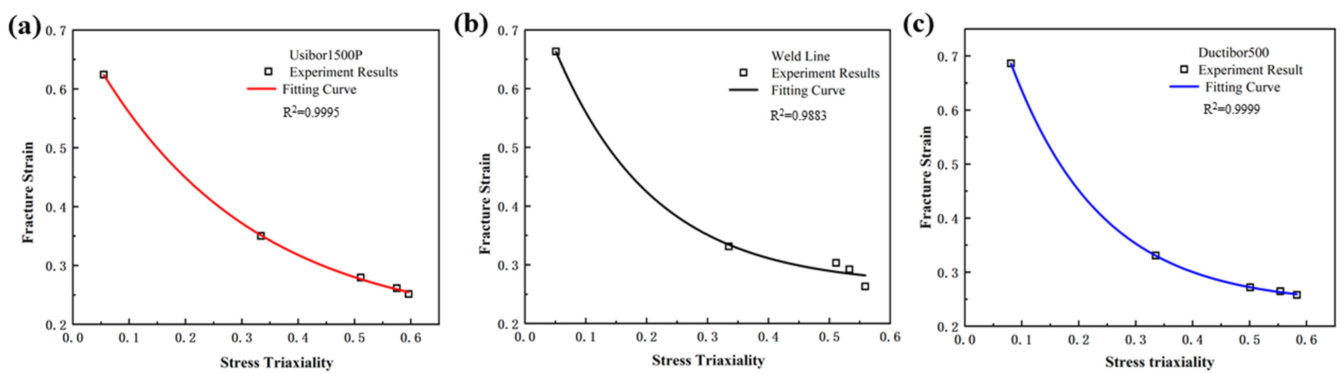
Figure 15.
The Fitting Relationship Curve between Stress Triaxiality and Fracture Strain: (a) Usibor1500P; (b) Weld seam; (c) Dustibor500.
Figure 15.
The Fitting Relationship Curve between Stress Triaxiality and Fracture Strain: (a) Usibor1500P; (b) Weld seam; (c) Dustibor500.
Figure 16.
Tensile test curves of smooth samples under different strain rates at room temperature: (a) Usibor1500P; (b) Weld seam; (c) Dustibor500.
Figure 16.
Tensile test curves of smooth samples under different strain rates at room temperature: (a) Usibor1500P; (b) Weld seam; (c) Dustibor500.
Figure 17.
Strain rate and fracture strain relationship curve: (a) Usibor1500P; (b) Weld seam; (c) Dustibor500.
Figure 17.
Strain rate and fracture strain relationship curve: (a) Usibor1500P; (b) Weld seam; (c) Dustibor500.
Figure 18.
True stress–strain curves of smooth samples under static tensile conditions at different temperatures: (a) Usibor1500P; (b) weld seam; (c) Dustibor500.
Figure 18.
True stress–strain curves of smooth samples under static tensile conditions at different temperatures: (a) Usibor1500P; (b) weld seam; (c) Dustibor500.
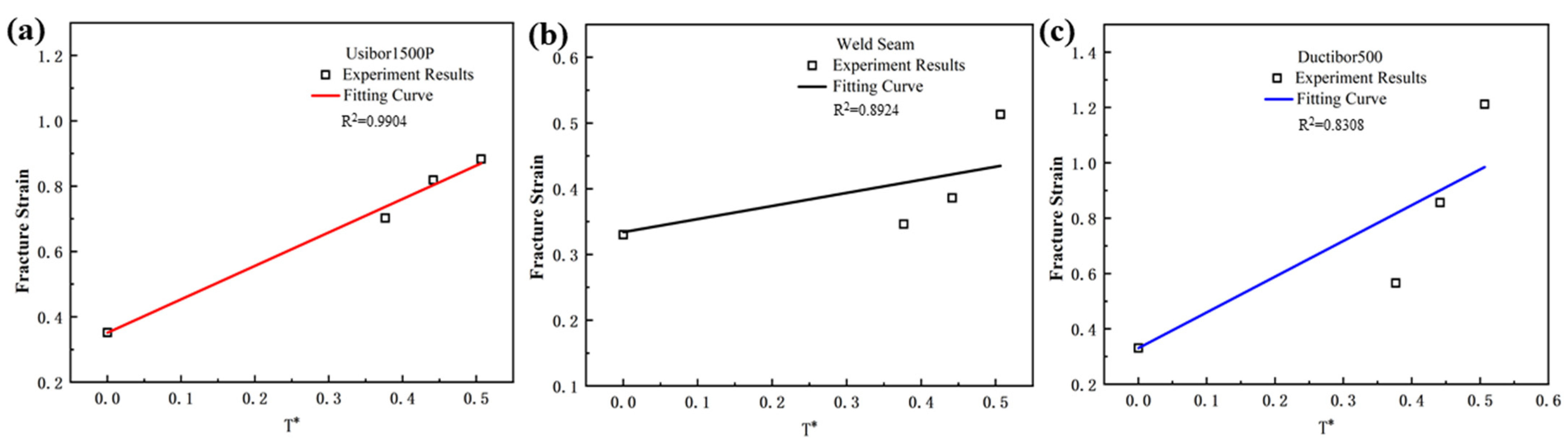
Figure 19.
The relationship curve between temperature and fracture strain: (a) Usibor1500P; (b) weld seam; (c) Dustibor500.
Figure 19.
The relationship curve between temperature and fracture strain: (a) Usibor1500P; (b) weld seam; (c) Dustibor500.
Figure 20.
SEM fracture topography weld seam×1000 ( s−1). Following features are marked: D—Dimple, R—River pattern, I—Inclusion, P—Porosity defect.
Figure 20.
SEM fracture topography weld seam×1000 ( s−1). Following features are marked: D—Dimple, R—River pattern, I—Inclusion, P—Porosity defect.
Figure 21.
Comparison between the numerical simulation and experimental results of tensile testing for welded specimens: (a) smooth specimen; (b) R2 notched specimen; (c) R5 notched specimen; (d) R8 notched specimen.
Figure 21.
Comparison between the numerical simulation and experimental results of tensile testing for welded specimens: (a) smooth specimen; (b) R2 notched specimen; (c) R5 notched specimen; (d) R8 notched specimen.
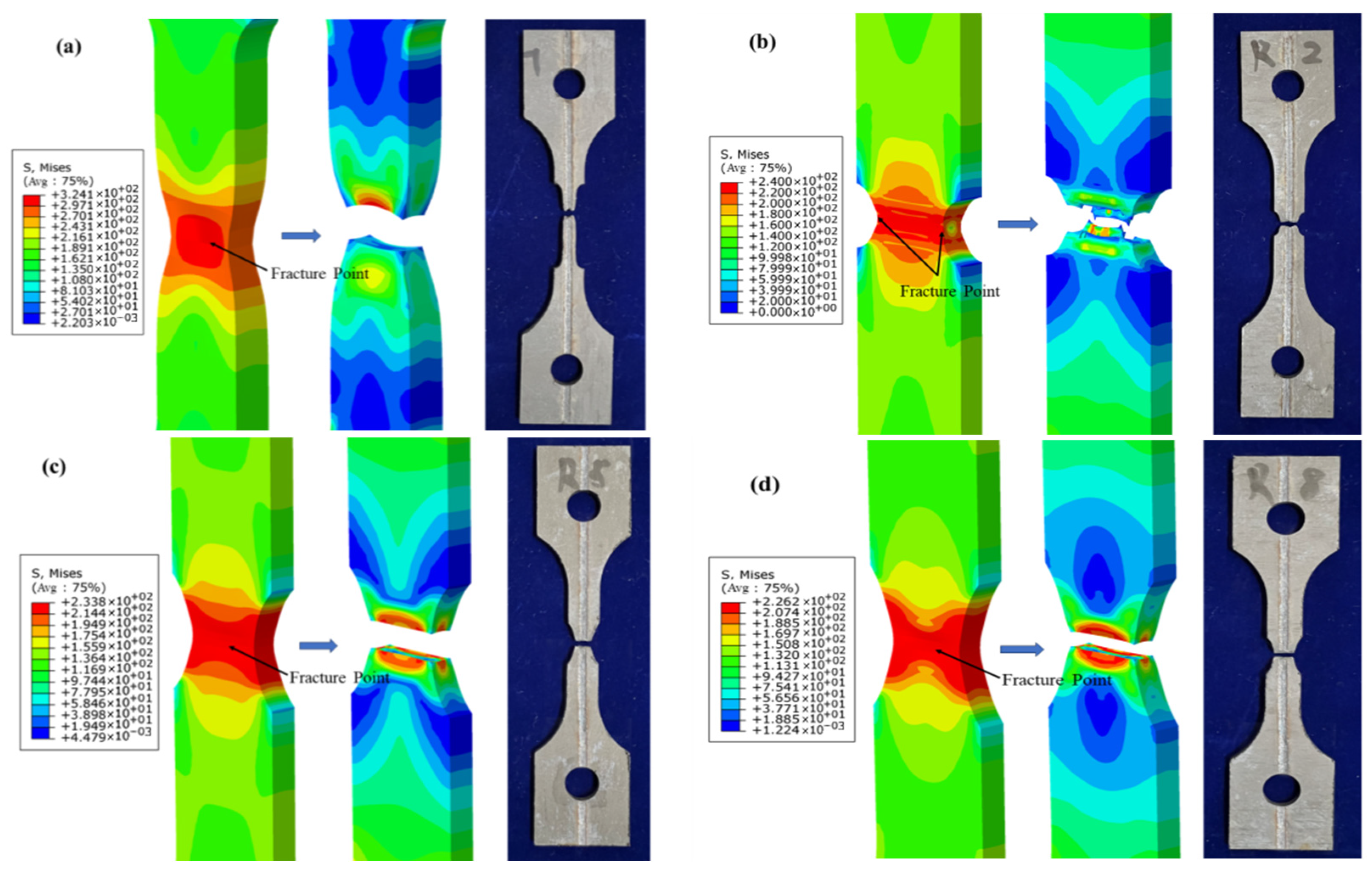
Figure 22.
Simulation results of the PEEQ at the fracture initiation point of tensile testing for welded specimens: (a) smooth specimen; (b) R2 notched specimen; (c) R5 notched specimen; (d) R8 notched specimen.
Figure 22.
Simulation results of the PEEQ at the fracture initiation point of tensile testing for welded specimens: (a) smooth specimen; (b) R2 notched specimen; (c) R5 notched specimen; (d) R8 notched specimen.
Figure 23.
Comparison of Load–Displacement Curves Between High-Strength Steel Usibor1500P Tensile Test and J–C Simulation; (a) Smooth specimen; (b) Notched Specimens.
Figure 23.
Comparison of Load–Displacement Curves Between High-Strength Steel Usibor1500P Tensile Test and J–C Simulation; (a) Smooth specimen; (b) Notched Specimens.
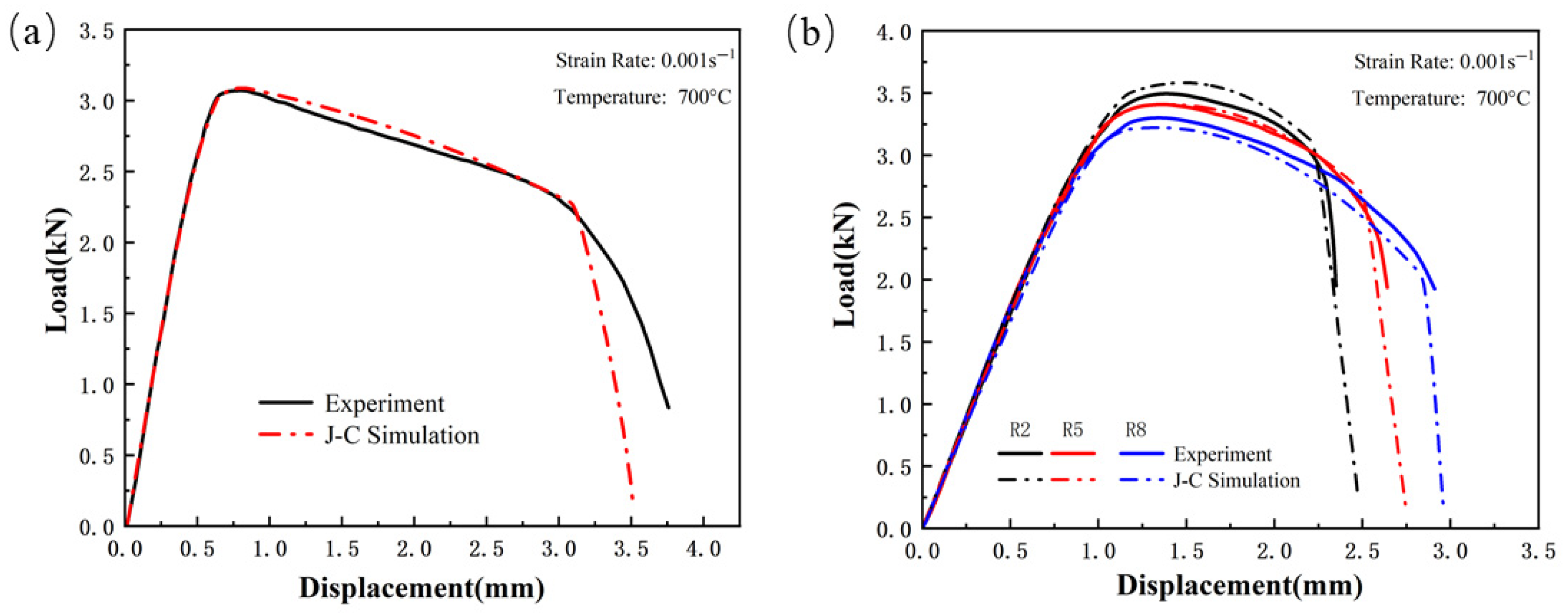
Figure 24.
Comparison of Load–Displacement Curves Between Weld Seam Tensile Test and J–C Simulation: (a) Smooth specimen; (b) Notched Specimens.
Figure 24.
Comparison of Load–Displacement Curves Between Weld Seam Tensile Test and J–C Simulation: (a) Smooth specimen; (b) Notched Specimens.
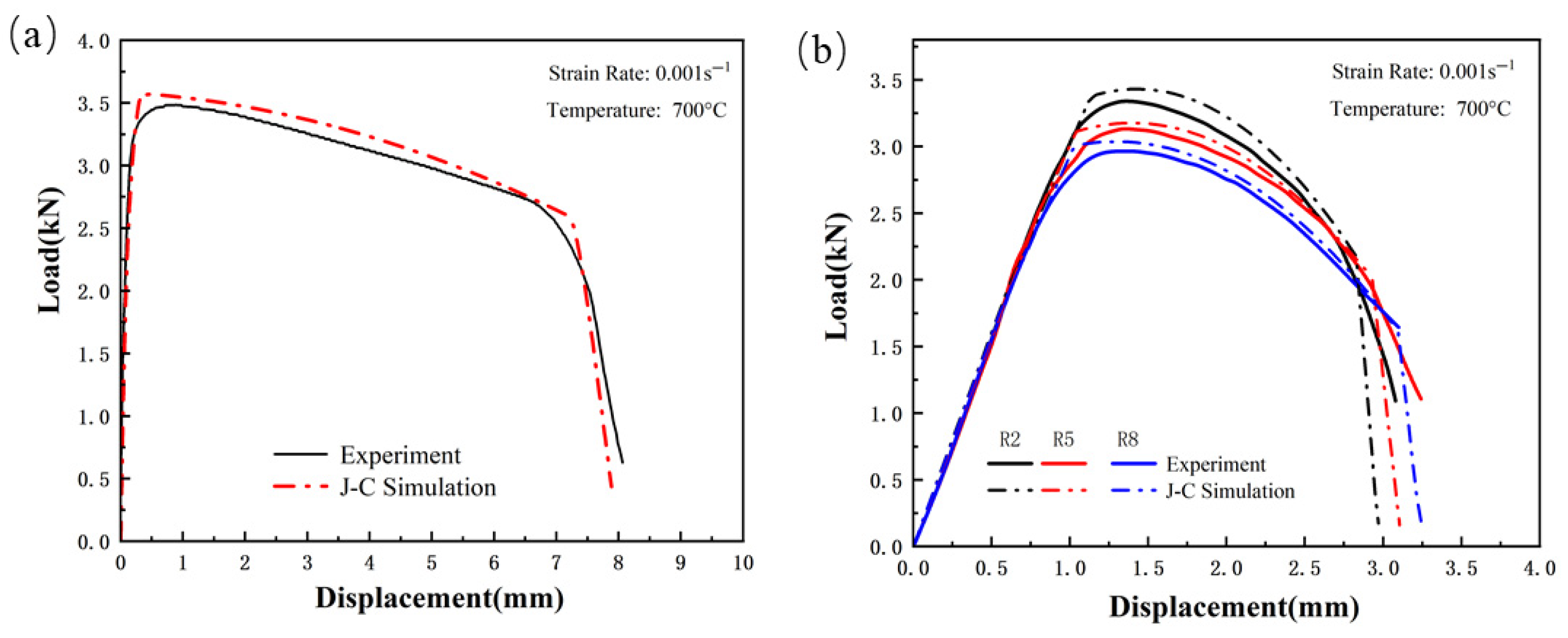
Figure 25.
Comparison of Load–Displacement Curves Between High-Strength Steel Ductibor500 Tensile Test and J–C Simulation; (a) Smooth specimen; (b) Notched Specimens.
Figure 25.
Comparison of Load–Displacement Curves Between High-Strength Steel Ductibor500 Tensile Test and J–C Simulation; (a) Smooth specimen; (b) Notched Specimens.
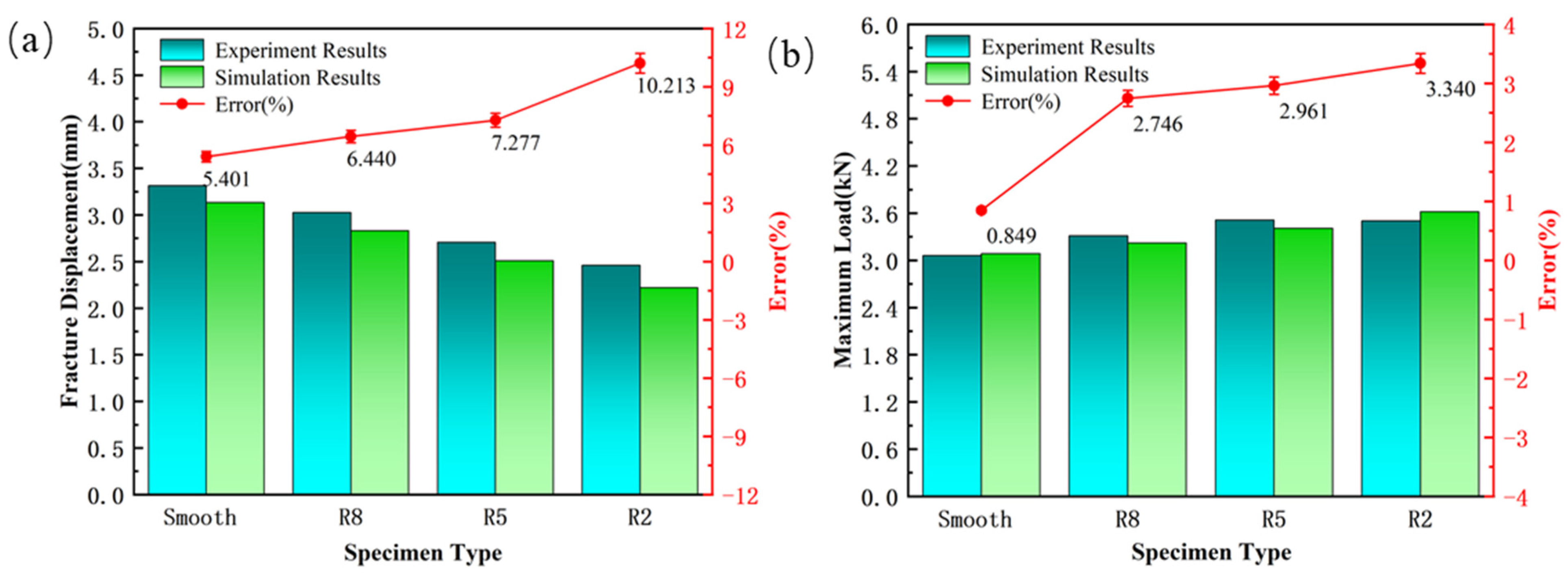
Figure 26.
Comparison of J–C Model Predicted Fracture Displacement and Maximum Load with Experimental Results and Corresponding Error Curves: (a) Fracture Displacement; (b) Maximum Load.
Figure 26.
Comparison of J–C Model Predicted Fracture Displacement and Maximum Load with Experimental Results and Corresponding Error Curves: (a) Fracture Displacement; (b) Maximum Load.
Figure 27.
Fracture Strain and Displacement vs. Stress Triaxiality Relationship Curve at Final Fracture of the First Failure Element.
Figure 27.
Fracture Strain and Displacement vs. Stress Triaxiality Relationship Curve at Final Fracture of the First Failure Element.
Figure 28.
Geometry and measurements of the hot Nakajima-type bulging test specimen.
Figure 28.
Geometry and measurements of the hot Nakajima-type bulging test specimen.
Figure 29.
Finite element model for hot Nakajima-type bulging tests of TWBs.
Figure 29.
Finite element model for hot Nakajima-type bulging tests of TWBs.
Figure 30.
FLD of Experimental Data and Simulation Results.
Figure 30.
FLD of Experimental Data and Simulation Results.
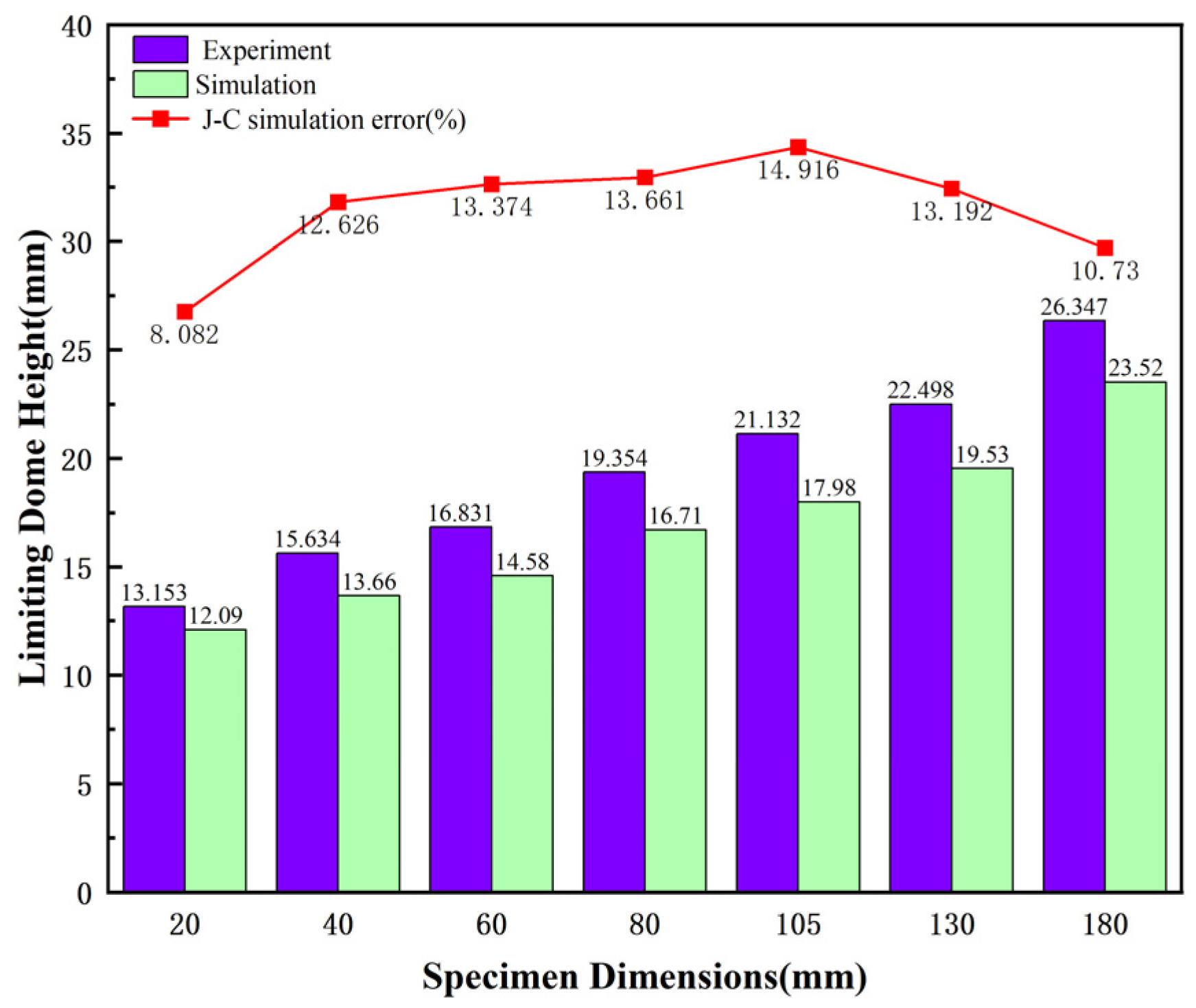
Figure 31.
Comparison of the limiting dome height at the point of specimen failure.
Figure 31.
Comparison of the limiting dome height at the point of specimen failure.
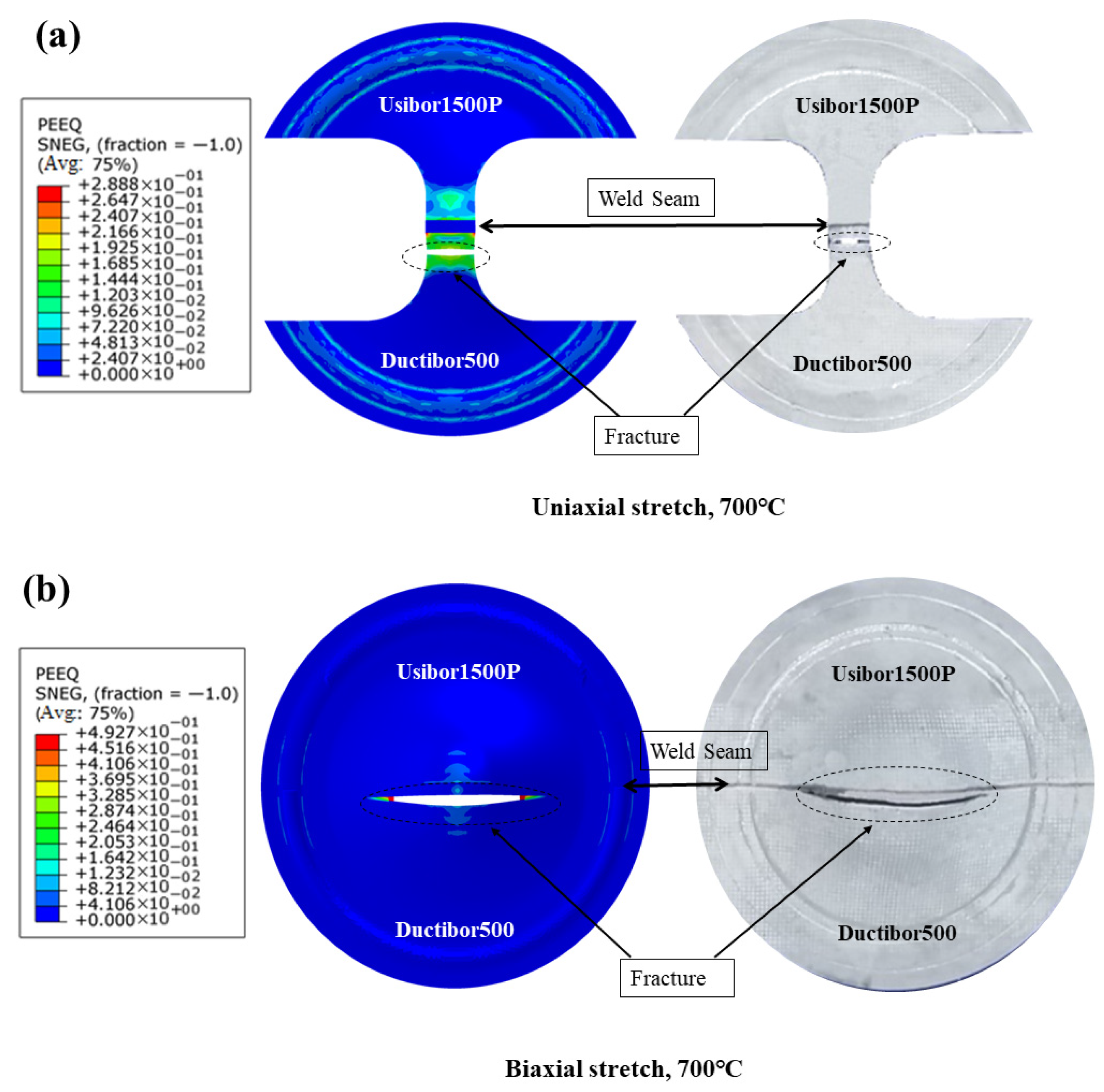
Figure 32.
Comparison of fractured specimens from simulation and experimental tests: (a) uniaxial tension state; (b) biaxial tension state.
Figure 32.
Comparison of fractured specimens from simulation and experimental tests: (a) uniaxial tension state; (b) biaxial tension state.
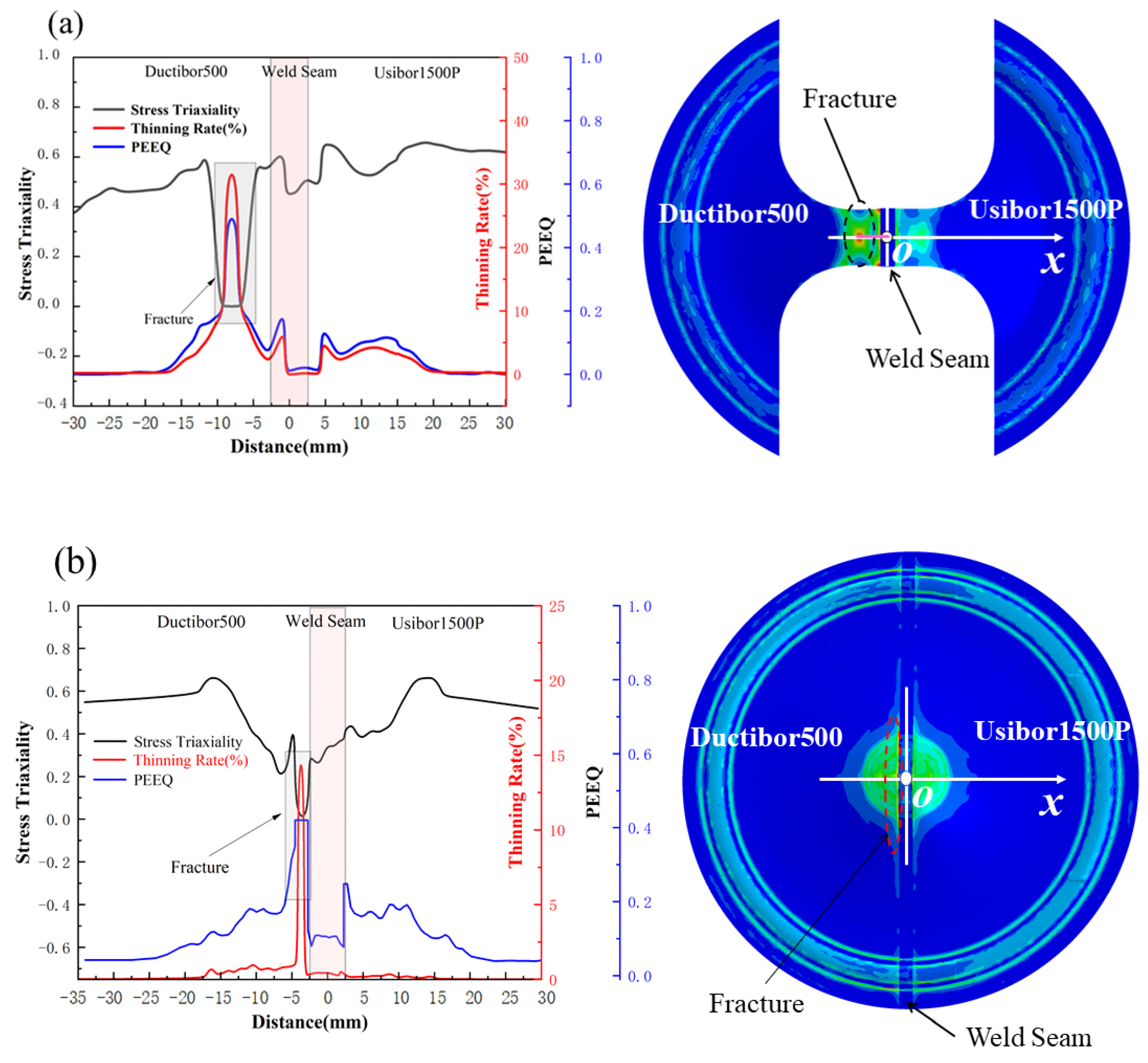
Figure 33.
Distribution of stress triaxiality, PEEQ, and thinning rate along the x-axis direction at the point of fracture of the specimen: (a) uniaxial tension state; (b) biaxial tension state.
Figure 33.
Distribution of stress triaxiality, PEEQ, and thinning rate along the x-axis direction at the point of fracture of the specimen: (a) uniaxial tension state; (b) biaxial tension state.
Table 1.
Experimental plan for determining the J–C damage model parameters.
Table 1.
Experimental plan for determining the J–C damage model parameters.
| Experimental Design | Temperature (°C) | Strain Rate | Model Parameters |
|---|
| Shear Specimens | Room Temperature | 0.001 s−1 | |
| Smooth Specimens | Room Temperature | 0.001 s−1 | D1, D2, D3 |
| Notched Specimens | Room Temperature | 0.001 s−1 | |
| Smooth Specimens | Room Temperature | 0.01 s−1, 0.05 s−1, 0.1 s−1 | D4 |
| Smooth Specimens | 600 °C, 700 °C, 800 °C | 0.001 s−1 | D5 |
Table 2.
Chemical composition of Usibor1500P (wt%).
Table 2.
Chemical composition of Usibor1500P (wt%).
| C | Si | Mn | Cr | Mo | P | S | Ti | Al | B |
|---|
| 0.20–0.25 | 0.15–0.35 | 1.10–1.40 | 0.15–0.30 | ≤0.35 | ≤0.025 | ≤0.008 | 0.020–0.050 | 0.020–0.060 | 0.002–0.004 |
Table 3.
Chemical composition of Ductibor500 (wt%).
Table 3.
Chemical composition of Ductibor500 (wt%).
| C | Si | Mn | P | S | Ti | Nb | Al | B |
|---|
| ≤0.10 | ≤0.50 | ≤1.90 | ≤0.030 | ≤0.025 | ≤0.150 | ≤0.090 | >0.015 | ≤0.001 |
Table 4.
Stress triaxiality and fracture strain of each specimen.
Table 4.
Stress triaxiality and fracture strain of each specimen.
| Specimen Type | Temperature (°C) | Strain Rate (s−1) | Usibor1500P | Weld Seam | Ductibor500 |
|---|
| | | | | |
|---|
| Shear | 20 | 0.001 | 0.055 | 0.624 | 0.051 | 0.663 | 0.081 | 0.6860 |
| Smooth | 20 | 0.001 | 0.334 | 0.3502 | 0.335 | 0.331 | 0.335 | 0.3305 |
| R2 | 20 | 0.001 | 0.596 | 0.2512 | 0.559 | 0.263 | 0.583 | 0.2578 |
| R5 | 20 | 0.001 | 0.575 | 0.2613 | 0.533 | 0.292 | 0.554 | 0.2646 |
| R8 | 20 | 0.001 | 0.511 | 0.2793 | 0.511 | 0.303 | 0.501 | 0.2717 |
Table 5.
J–C damage model parameters (D1, D2 and D3) of different regions.
Table 5.
J–C damage model parameters (D1, D2 and D3) of different regions.
| Region | D1 | D2 | D3 |
|---|
| Usibor1500P | 0.1926 | 0.5253 | −3.5847 |
| Weld Seam | 0.264 | 0.545 | −6.1223 |
| Ductibor500 | 0.24 | 0.7415 | −6.2775 |
Table 6.
Stress triaxiality and fracture strain of smooth samples under different strain rate conditions.
Table 6.
Stress triaxiality and fracture strain of smooth samples under different strain rate conditions.
| Specimen Type | Temperature (°C) | Strain Rate (s−1) | Usibor1500P | Weld Seam | Ductibor500 |
|---|
| | | | | |
|---|
| Smooth | 20 | 0.001 | 0.334 | 0.3502 | 0.335 | 0.331 | 0.335 | 0.3305 |
| Smooth | 20 | 0.01 | 0.334 | 0.2987 | 0.335 | 0.218 | 0.335 | 0.234 |
| Smooth | 20 | 0.05 | 0.334 | 0.2678 | 0.335 | 0.193 | 0.335 | 0.2033 |
| Smooth | 20 | 0.1 | 0.334 | 0.2475 | 0.335 | 0.181 | 0.335 | 0.188 |
Table 7.
J–C damage model parameters (D1, D2, D3 and D4) of different regions.
Table 7.
J–C damage model parameters (D1, D2, D3 and D4) of different regions.
| Region | D1 | D2 | D3 | D4 |
|---|
| Usibor1500P | 0.1926 | 0.5253 | −3.5847 | −0.063 |
| Weld Seam | 0.264 | 0.545 | −6.1223 | −0.109 |
| Ductibor500 | 0.24 | 0.7415 | −6.2775 | −0.0996 |
Table 8.
Stress triaxiality and fracture strain of smooth samples under different temperature conditions.
Table 8.
Stress triaxiality and fracture strain of smooth samples under different temperature conditions.
| Specimen Type | Temperature (°C) | Strain Rate (s−1) | Usibor1500P | Weld Seam | Ductibor500 |
|---|
| | | | | |
|---|
| Smooth | 600 | 0.001 | 0.334 | 0.7018 | 0.335 | 0.346 | 0.335 | 0.5649 |
| Smooth | 700 | 0.001 | 0.334 | 0.8182 | 0.335 | 0.386 | 0.335 | 0.8560 |
| Smooth | 800 | 0.001 | 0.334 | 0.8828 | 0.335 | 0.513 | 0.335 | 1.2110 |
Table 9.
J–C damage model parameters of different regions.
Table 9.
J–C damage model parameters of different regions.
| Region | D1 | D2 | D3 | D4 | D5 |
|---|
| Usibor1500P | 0.1926 | 0.5253 | −3.5847 | −0.063 | 2.914 |
| Weld Seam | 0.264 | 0.545 | −6.1223 | −0.109 | 0.596 |
| Ductibor500 | 0.24 | 0.7415 | −6.2775 | −0.0996 | 3.907 |
Table 10.
Thermophysical properties at various temperatures [
38,
39,
40].
Table 10.
Thermophysical properties at various temperatures [
38,
39,
40].
| Temperature (°C) | 20 | 200 | 400 | 600 | 800 |
|---|
| Ductibor500 | | | | | |
| Specific heat (J/kg/°C) | 506 | 515 | 523 | 534 | 546 |
| Conductivity (W/m/°C) | 50 | 48 | 46 | 44 | 42 |
| Expansion coefficient (μm/m/°C) | 12.5 | 13.0 | 14.5 | 15.0 | 16.5 |
| weld seam | | | | | |
| Specific heat (J/kg/°C) | 460 | 500 | 550 | 600 | 650 |
| Conductivity (W/m/°C) | 35 | 30 | 25 | 20 | 15 |
| Expansion coefficient (μm/m/°C) | 12.0 | 12.5 | 13.0 | 13.5 | 14.0 |
| Usibor1500P | | | | | |
| Specific heat (J/kg/°C) | 481 | 493 | 502 | 511 | 522 |
| Conductivity (W/m/°C) | 45 | 43 | 41 | 39 | 37 |
| Expansion coefficient (μm/m/°C) | 11.4 | 12.6 | 13.0 | 14.5 | 15.5 |


