

Use of BOIvy Optimization Algorithm-Based Machine Learning Models in Predicting the Compressive Strength of Bentonite Plastic Concrete


Abstract
1. Introduction
2. Methodologies
2.1. SVR
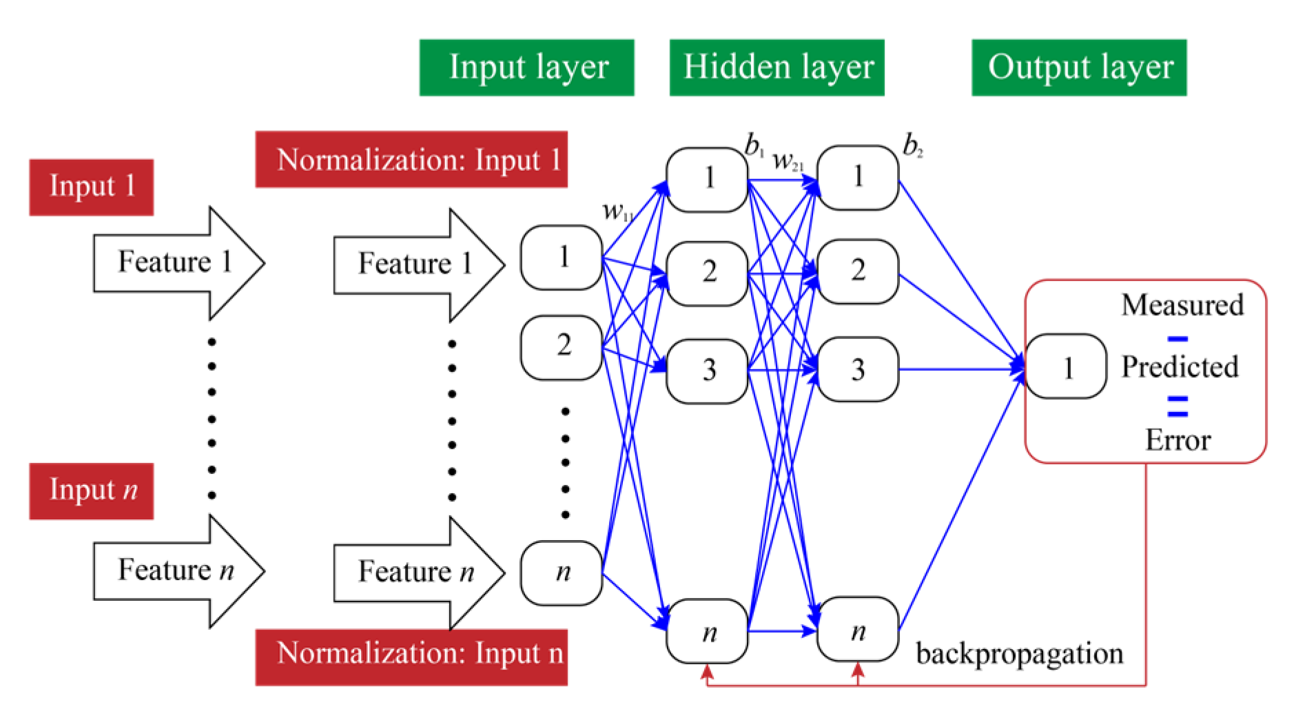
2.2. ANN
2.3. RF
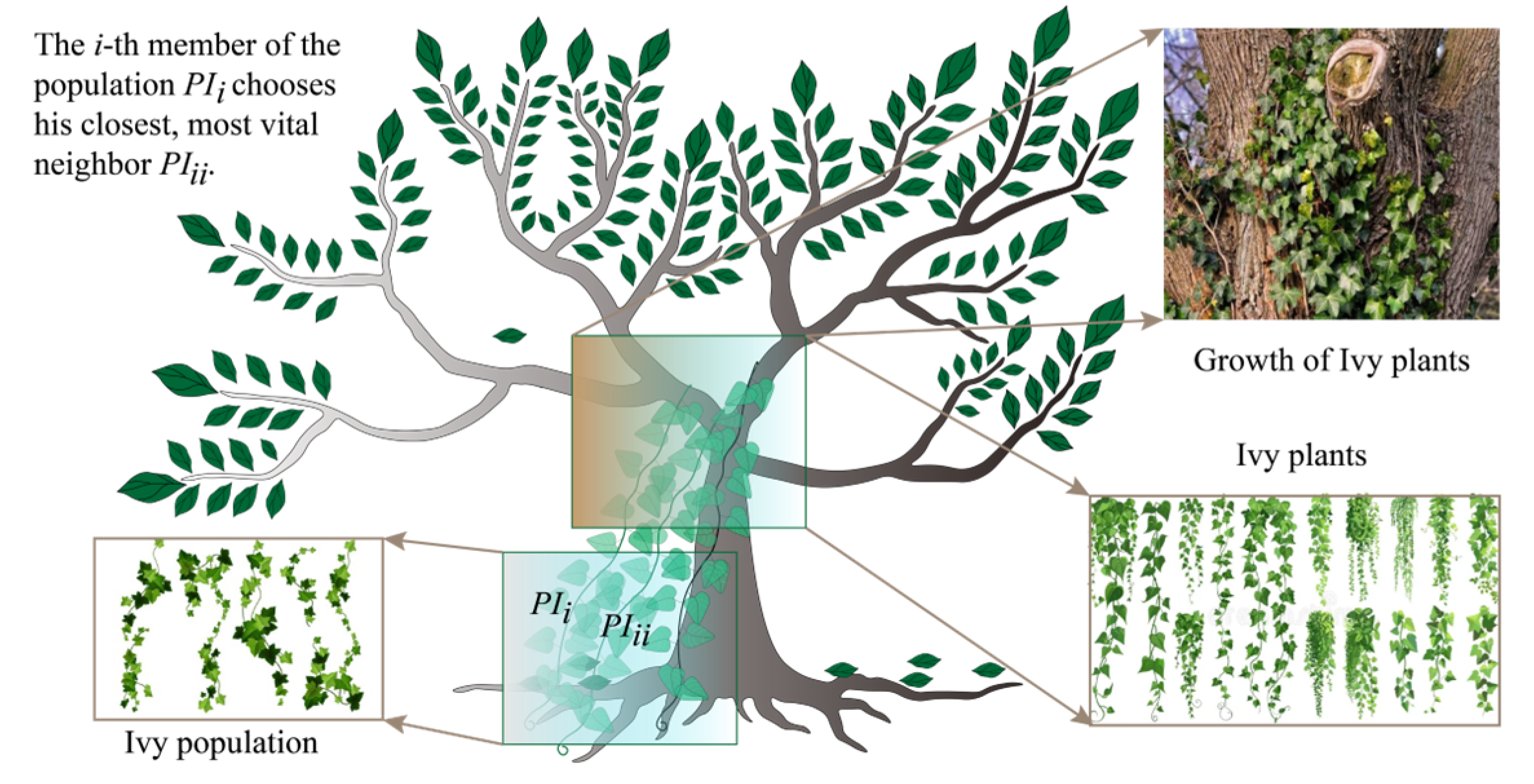
2.4. Ivy Algorithm with Bayesian Optimization
- (1)
- Population initialization
- (2)
- Population growth
- (3)
- Growth with sunlight
- (4)
- Spreading and evolution
| Algorithm 1 Pseudo-code of BO-enhanced Ivy initialization. |
| Input Initialize dataset D = {} for t in range (1, T + 1): if t == 1: x_t = RandomSample () else: Fit GP model on D Define acquisition function (expected improvement) x_t = argmax_x AcquisitionFunction(x) y_t = EvaluateObjectiveFunction (x_t) D = D ∪ {(x_t, y_t)} TopCandidates = SelectTopK (D, k) InitializeIvyPopulation (TopCandidates) RunIvyOptimization() End |
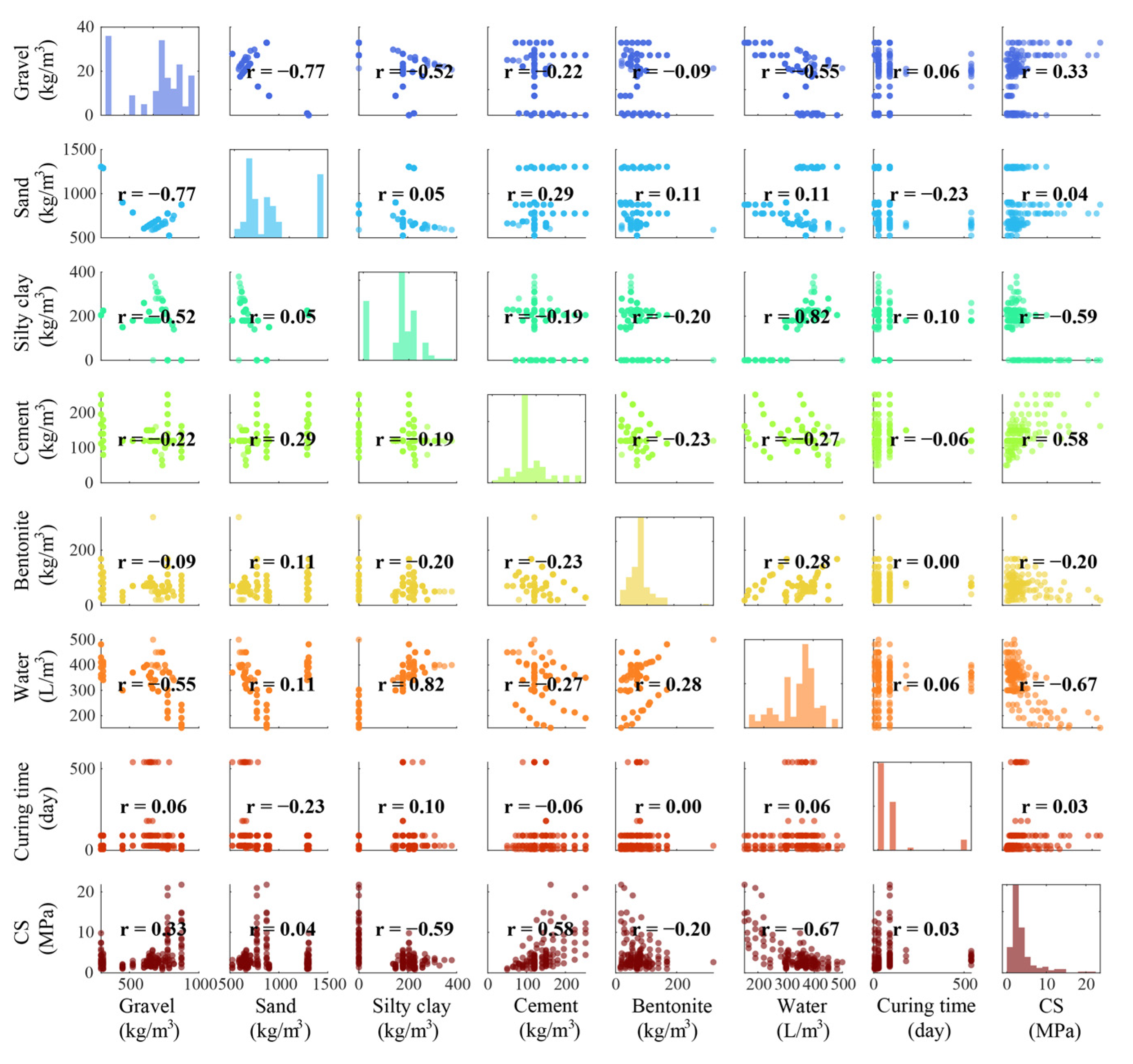
3. Database
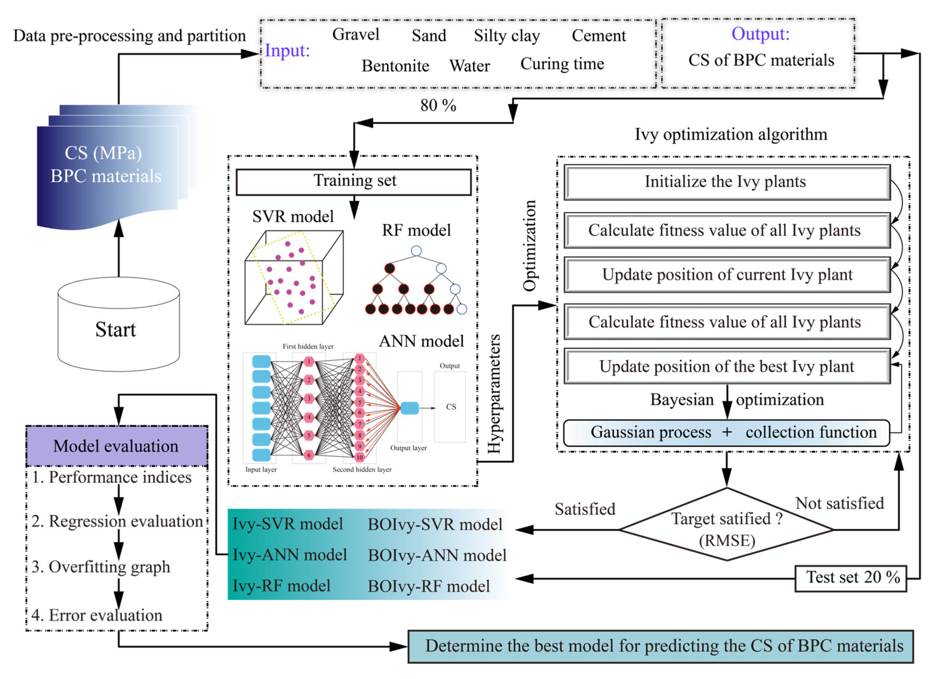
4. Development of Prediction Models
- (1)
- Data preparation
- (2)
- Hyperparameter optimization
- (3)
- Model evaluation
5. Results and Discussion
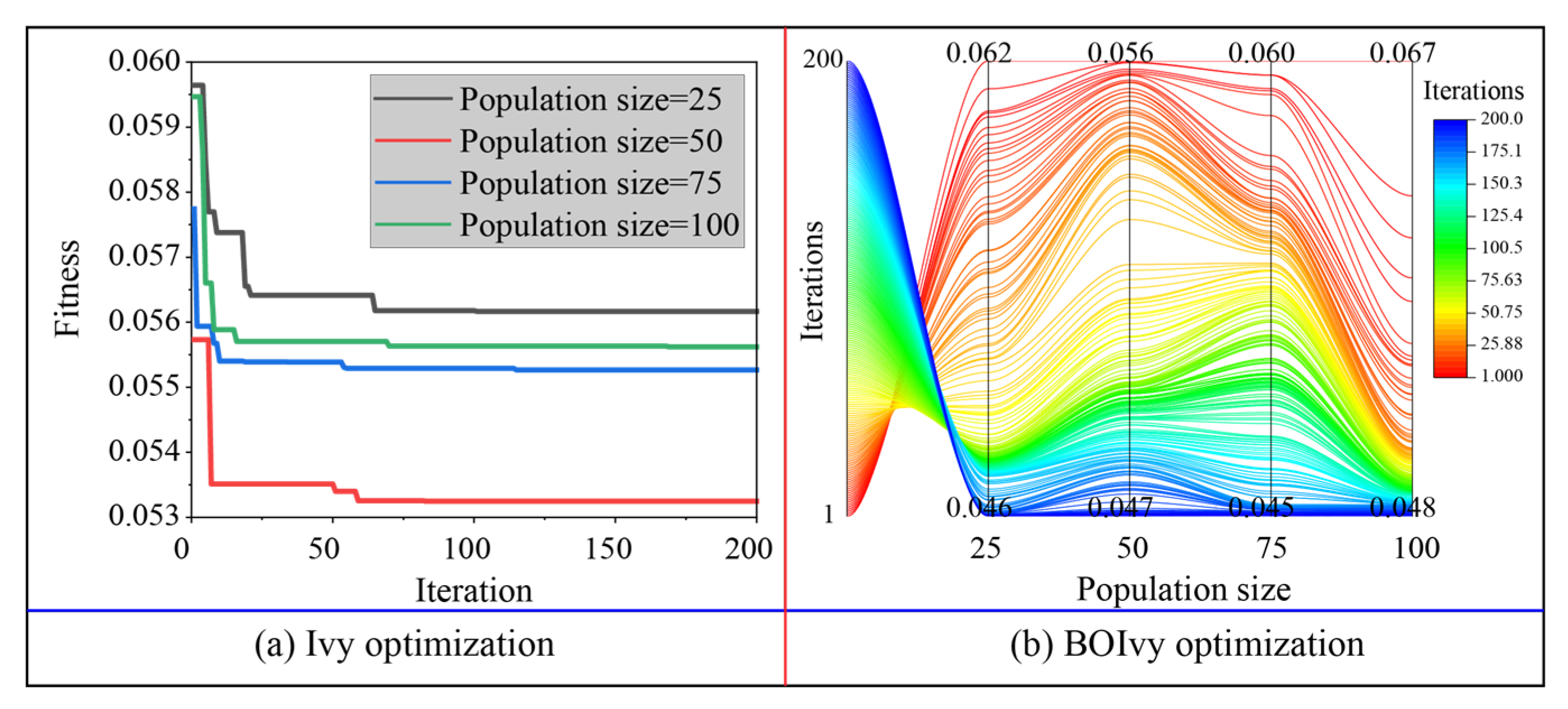
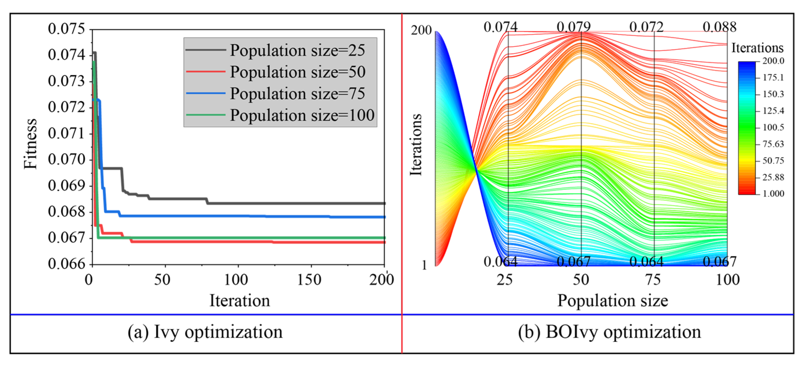
5.1. Model Optimization
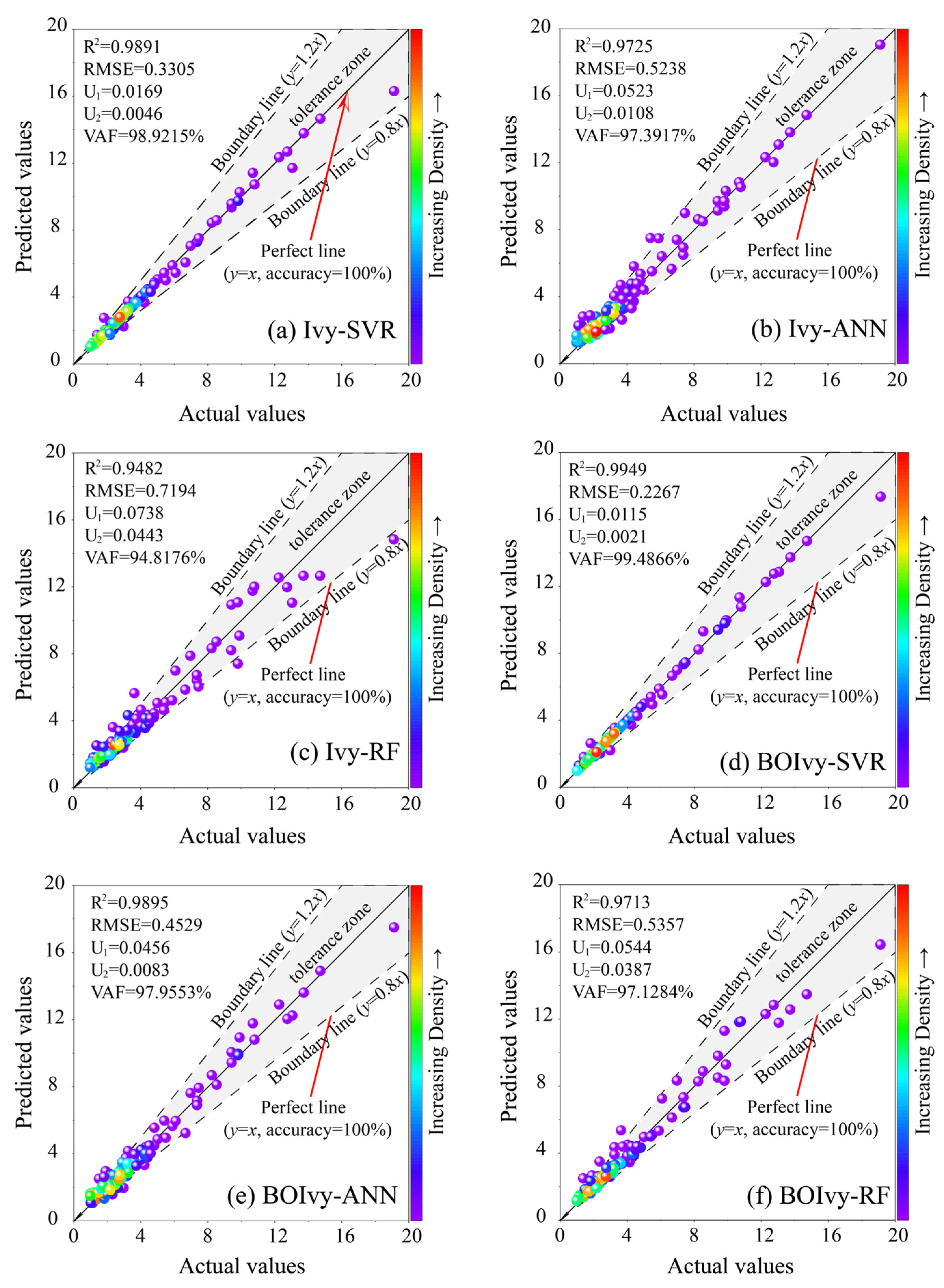
5.2. Model Performance Evaluation
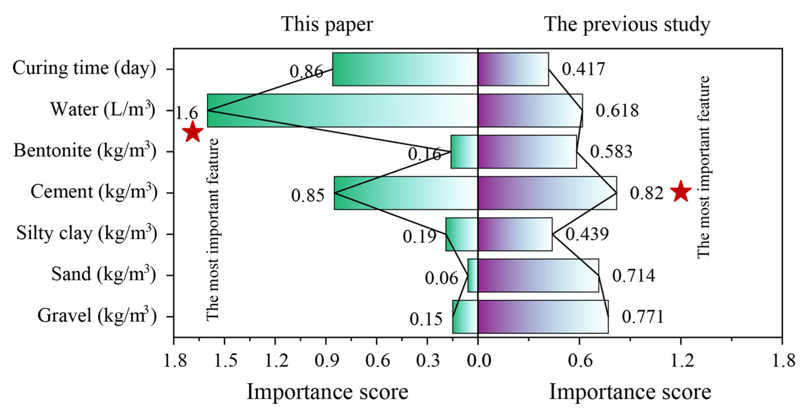
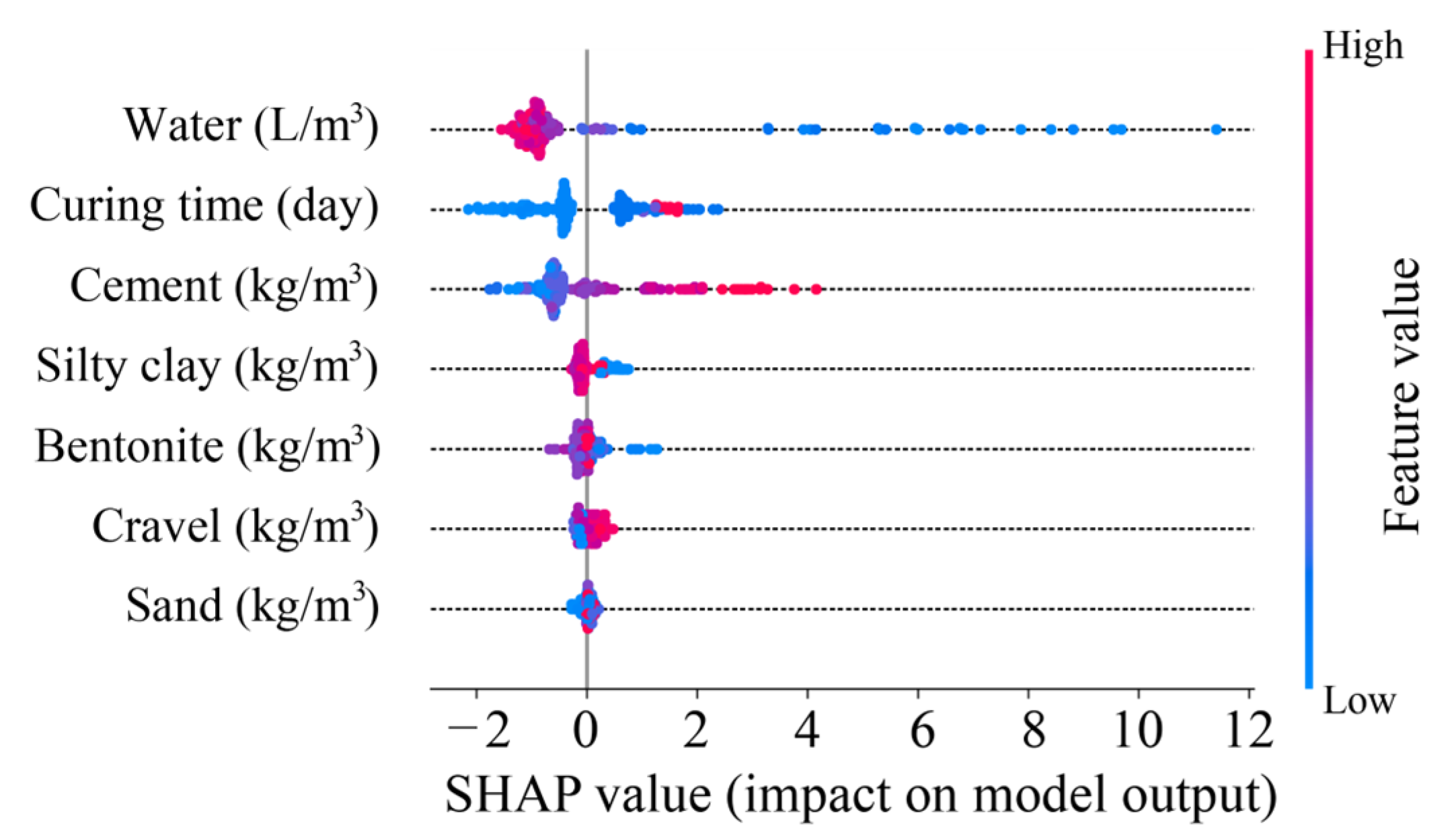
5.3. Model Interpretability
6. Conclusions
- (1)
- The results of model optimization indicated that BO significantly improved the optimization ability of the original Ivy algorithm, though the performance improvement for the RF model was relatively limited.
- (2)
- The results of the model evaluation demonstrated that the BOIvy-ANN model outperformed the other models in predicting the CS of BPC materials, achieving the optimal indices with the test set (R2: 0.9855, RMSE: 0.5998, U1: 0.0441, U2: 0.0077, and VAF: 98.5778%) and the lowest fitting evaluation indices (R2: −0.006, RMSE: −0.1469, U1: 0.0015, U2: 6 × 10⁻⁴, and VAF: −0.6225)
- (3)
- The results of the model explanation illustrated that water was the most important feature in predicting CS and had a negative contribution. Additionally, curing time and cement also played significant roles in CS prediction.
Author Contributions
Funding
Institutional Review Board Statement
Informed Consent Statement
Data Availability Statement
Acknowledgments
Conflicts of Interest
References
- Shepherd, D.A.; Kotan, E.; Dehn, F. Plastic concrete for cut-off walls: A review. Constr. Build. Mater. 2020, 255, 119248. [Google Scholar] [CrossRef]
- Abbaslou, H.; Ghanizadeh, A.R.; Amlashi, A.T. The compatibility of bentonite/sepiolite plastic concrete cut-off wall material. Constr. Build. Mater. 2016, 124, 1165–1173. [Google Scholar] [CrossRef]
- Mousavi, S.S.; Bhojaraju, C.; Ouellet-Plamondon, C. Clay as a sustainable binder for concrete—A review. Constr. Mater. 2021, 1, 134–168. [Google Scholar] [CrossRef]
- Saikia, N.; De Brito, J. Use of plastic waste as aggregate in cement mortar and concrete preparation: A review. Constr. Build. Mater. 2012, 34, 385–401. [Google Scholar] [CrossRef]
- Koch, D. Bentonites as a basic material for technical base liners and site encapsulation cut-off walls. Appl. Clay Sci. 2002, 21, 1–11. [Google Scholar] [CrossRef]
- Dhar, A.K.; Himu, H.A.; Bhattacharjee, M.; Mostufa, M.G.; Parvin, F. Insights on applications of bentonite clays for the removal of dyes and heavy metals from wastewater: A review. Environ. Sci. Pollut. Res. 2023, 30, 5440–5474. [Google Scholar] [CrossRef]
- Thapa, I.; Kumar, N.; Ghani, S.; Kumar, S.; Gupta, M. Applications of bentonite in plastic concrete: A comprehensive study on enhancing workability and predicting compressive strength using hybridized AI models. Asian J. Civ. Eng. 2024, 25, 3113–3128. [Google Scholar] [CrossRef]
- Mahboubi, A.; Ajorloo, A. Experimental study of the mechanical behavior of plastic concrete in triaxial compression. Cem. Concr. Res. 2005, 35, 412–419. [Google Scholar] [CrossRef]
- Kazemian, S.; Ghareh, S.; Torkanloo, L. To investigation of plastic concrete bentonite changes on it’s physical properties. Procedia Eng. 2016, 145, 1080–1087. [Google Scholar] [CrossRef]
- Iravanian, A.; Bilsel, H. Tensile strength properties of sand-bentonite mixtures enhanced with cement. Procedia Eng. 2016, 143, 111–118. [Google Scholar] [CrossRef]
- Shepherd, D.A.; Dehn, F. Experimental study into the mechanical properties of plastic concrete: Compressive strength development over time, tensile strength and elastic modulus. Case Stud. Constr. Mater. 2023, 19, e02521. [Google Scholar] [CrossRef]
- Kazemian, S.; Ghareh, S. Effects of Cement, Different Bentonite, and Aggregates on Plastic Concrete in Besh-Ghardash Dam, Iran. J. Test. Eval. 2017, 45, 242–248. [Google Scholar] [CrossRef]
- Haq, I.U.; Elahi, A.; Nawaz, A.; Shah, S.A.Q.; Ali, K. Mechanical and durability performance of concrete mixtures incorporating bentonite, silica fume, and polypropylene fibers. Constr. Build. Mater. 2022, 345, 128223. [Google Scholar] [CrossRef]
- Tang, B.; Cui, W.; Zhang, B.Z.; Jiang, Z.A. The macroscopic mechanical characteristics and microscopic evolution mechanism of plastic concrete. Constr. Build. Mater. 2023, 391, 131898. [Google Scholar] [CrossRef]
- Iravanian, A.; Bilsel, H. Strength characterization of sand-bentonite mixtures and the effect of cement additives. Mar. Georesources Geotechnol. 2016, 34, 210–218. [Google Scholar] [CrossRef]
- Basha, A.; Mansour, W. Variation of the hydraulic conductivity and the mechanical characteristics of plastic concrete with time. Int. J. Concr. Struct. Mater. 2023, 17, 27. [Google Scholar] [CrossRef]
- Iftikhar, B.; Alih, S.C.; Vafaei, M.; Javed, M.F.; Rehman, M.F.; Abdullaev, S.S.; Tamam, N.; Khan, M.I.; Hassan, A.M. Predicting compressive strength of eco-friendly plastic sand paver blocks using gene expression and artificial intelligence programming. Sci. Rep. 2023, 13, 12149. [Google Scholar] [CrossRef]
- Alaneme, G.U.; Mbadike, E.M. Optimisation of strength development of bentonite and palm bunch ash concrete using fuzzy logic. Int. J. Sustain. Eng. 2021, 14, 835–851. [Google Scholar] [CrossRef]
- Zhou, C.; Rui, Y.; Qiu, J.; Wang, Z.; Zhou, T.; Long, X.; Shan, K. The role of fracture in dynamic tensile responses of fractured rock mass: Insight from a particle-based model. Int. J. Coal Sci. Technol. 2025, 12, 39. [Google Scholar] [CrossRef]
- Li, C.; Zhou, J.; Tao, M.; Du, K.; Wang, S.; Armaghani, D.J.; Mohamad, E.T. Developing hybrid ELM-ALO, ELM-LSO and ELM-SOA models for predicting advance rate of TBM. Transp. Geotech. 2022, 36, 100819. [Google Scholar] [CrossRef]
- Li, C.; Zhou, J.; Dias, D.; Gui, Y. A kernel extreme learning machine-grey wolf optimizer (KELM-GWO) model to predict uniaxial compressive strength of rock. Appl. Sci. 2022, 12, 8468. [Google Scholar] [CrossRef]
- Tapeh, A.T.G.; Naser, M.Z. Artificial intelligence, machine learning, and deep learning in structural engineering: A scientometrics review of trends and best practices. Arch. Comput. Methods Eng. 2023, 30, 115–159. [Google Scholar] [CrossRef]
- Paudel, S.; Pudasaini, A.; Shrestha, R.K.; Kharel, E. Compressive strength of concrete material using machine learning techniques. Clean. Eng. Technol. 2023, 15, 100661. [Google Scholar] [CrossRef]
- Ziolkowski, P.; Niedostatkiewicz, M. Machine learning techniques in concrete mix design. Materials 2019, 12, 1256. [Google Scholar] [CrossRef]
- Zhou, J.; Li, E.; Wei, H.; Li, C.; Qiao, Q.; Armaghani, D.J. Random forests and cubist algorithms for predicting shear strengths of rockfill materials. Appl. Sci. 2019, 9, 1621. [Google Scholar] [CrossRef]
- Inqiad, W.B.; Javed, M.F.; Onyelowe, K.; Siddique, M.S.; Asif, U.; Alkhattabi, L.; Aslam, F. Soft computing models for prediction of bentonite plastic concrete strength. Sci. Rep. 2024, 14, 18145. [Google Scholar] [CrossRef]
- Ghanizadeh, A.R.; Abbaslou, H.; Amlashi, A.T.; Alidoust, P. Modeling of bentonite/sepiolite plastic concrete compressive strength using artificial neural network and support vector machine. Front. Struct. Civ. Eng. 2019, 13, 215–239. [Google Scholar] [CrossRef]
- Khan, M.; Ali, M.; Najeh, T.; Gamil, Y. Computational prediction of workability and mechanical properties of bentonite plastic concrete using multi-expression programming. Sci. Rep. 2024, 14, 6105. [Google Scholar] [CrossRef]
- Alishvandi, A.; Karimi, J.; Damari, S.; Moayedi Far, A.; Setodeh Pour, M.; Ahmadi, M. Estimating the compressive strength of plastic concrete samples using machine learning algorithms. Asian J. Civ. Eng. 2024, 25, 1503–1516. [Google Scholar] [CrossRef]
- Kumar, P.; Shekhar Kamal, S.; Kumar, A.; Kumar, N.; Kumar, S. Compressive strength of bentonite concrete using state-of-the-art optimised XGBoost models. Nondestruct. Test. Eval. 2024, 1–24. [Google Scholar] [CrossRef]
- Li, C.; Zhou, J.; Armaghani, D.J.; Li, X. Stability analysis of underground mine hard rock pillars via combination of finite difference methods, neural networks, and Monte Carlo simulation techniques. Undergr. Space 2021, 6, 379–395. [Google Scholar] [CrossRef]
- Li, C.; Zhang, J.; Mei, X.; Zhou, J. Supervised intelligent prediction of shear strength of rockfill materials based on data driven and a case study. Transp. Geotech. 2024, 45, 101229. [Google Scholar] [CrossRef]
- Barreñada, L.; Dhiman, P.; Timmerman, D.; Boulesteix, A.L.; Van Calster, B. Understanding overfitting in random forest for probability estimation: A visualization and simulation study. Diagn. Progn. Res. 2024, 8, 14. [Google Scholar] [CrossRef] [PubMed]
- Shahriari, B.; Swersky, K.; Wang, Z.; Adams, R.P.; De Freitas, N. Taking the human out of the loop: A review of Bayesian optimization. Proc. IEEE 2015, 104, 148–175. [Google Scholar] [CrossRef]
- Wang, X.; Jin, Y.; Schmitt, S.; Olhofer, M. Recent advances in Bayesian optimization. ACM Comput. Surv. 2023, 55, 1–36. [Google Scholar] [CrossRef]
- Soares, R.C.; Silva, J.C.; de Lucena Junior, J.A.; Lima Filho, A.C.; de Souza Ramos, J.G.G.; Brito, A.V. Integration of Bayesian optimization into hyperparameter tuning of the particle swarm optimization algorithm to enhance neural networks in bearing failure classification. Measurement 2025, 242, 115829. [Google Scholar] [CrossRef]
- Amlashi, A.T.; Abdollahi, S.M.; Goodarzi, S.; Ghanizadeh, A.R. Soft computing based formulations for slump, compressive strength, and elastic modulus of bentonite plastic concrete. J. Clean. Prod. 2019, 230, 1197–1216. [Google Scholar] [CrossRef]
- Awad, M.; Khanna, R.; Awad, M.; Khanna, R. Support vector regression. In Efficient Learning Machines Theories, Concepts, and Applications for Engineers and System Designers; Apress: Berkeley, CA, USA, 2015; pp. 67–80. [Google Scholar]
- Liu, Q.; Chen, C.; Zhang, Y.; Hu, Z. Feature selection for support vector machines with RBF kernel. Artif. Intell. Rev. 2011, 36, 99–115. [Google Scholar] [CrossRef]
- Yong, W.; Zhang, W.; Nguyen, H.; Bui, X.N.; Choi, Y.; Nguyen-Thoi, T.; Zhou, J.; Tran, T.T. Analysis and prediction of diaphragm wall deflection induced by deep braced excavations using finite element method and artificial neural network optimized by metaheuristic algorithms. Reliab. Eng. Syst. Saf. 2022, 221, 108335. [Google Scholar] [CrossRef]
- Bourquin, J.; Schmidli, H.; van Hoogevest, P.; Leuenberger, H. Basic concepts of artificial neural networks (ANN) modeling in the application to pharmaceutical development. Pharm. Dev. Technol. 1997, 2, 95–109. [Google Scholar] [CrossRef]
- Dai, Y.; Khandelwal, M.; Qiu, Y.; Zhou, J.; Monjezi, M.; Yang, P. A hybrid metaheuristic approach using random forest and particle swarm optimization to study and evaluate backbreak in open-pit blasting. Neural Comput. Appl. 2022, 34, 6273–6288. [Google Scholar] [CrossRef]
- Ghasemi, M.; Zare, M.; Trojovský, P.; Rao, R.V.; Trojovská, E.; Kandasamy, V. Optimization based on the smart behavior of plants with its engineering applications: Ivy algorithm. Knowl.-Based Syst. 2024, 295, 111850. [Google Scholar] [CrossRef]
- Pelikan, M.; Pelikan, M. Bayesian optimization algorithm. In Hierarchical Bayesian Optimization Algorithm: Toward a New Generation of Evolutionary Algorithms; Springer: Berlin/Heidelberg, Germany, 2005; pp. 31–48. [Google Scholar]
- Maatouk, H.; Bay, X. Gaussian process emulators for computer experiments with inequality constraints. Math. Geosci. 2017, 49, 557–582. [Google Scholar] [CrossRef]
- Zhan, D.; Xing, H. Expected improvement for expensive optimization: A review. J. Glob. Optim. 2020, 78, 507–544. [Google Scholar] [CrossRef]
- Kannangara, K.P.M.; Zhou, W.; Ding, Z.; Hong, Z. Investigation of feature contribution to shield tunneling-induced settlement using Shapley additive explanations method. J. Rock Mech. Geotech. Eng. 2022, 14, 1052–1063. [Google Scholar] [CrossRef]
- Zhou, S.; Zhang, Z.X.; Luo, X.; Huang, Y.; Yu, Z.; Yang, X. Predicting dynamic compressive strength of frozen-thawed rocks by characteristic impedance and data-driven methods. J. Rock Mech. Geotech. Eng. 2024, 16, 2591–2606. [Google Scholar] [CrossRef]
- Naser, M.Z.; Alavi, A.H. Error metrics and performance fitness indicators for artificial intelligence and machine learning in engineering and sciences. Archit. Struct. Constr. 2023, 3, 499–517. [Google Scholar] [CrossRef]
- Li, J.; Li, C.; Zhang, S. Application of Six Metaheuristic Optimization Algorithms and Random Forest in the uniaxial compressive strength of rock prediction. Appl. Soft Comput. 2022, 131, 109729. [Google Scholar] [CrossRef]
- Nie, F.; Chow, C.L.; Lau, D. Molecular dynamics study on the cohesive fracture properties of functionalized styrene-butadiene rubber modified asphalt. Resour. Conserv. Recycl. 2024, 208, 107715. [Google Scholar] [CrossRef]
- Qiu, J.; Huang, R.; Wang, H.; Wang, F.; Zhou, C. Rate-dependent tensile behaviors of jointed rock masses considering geological conditions using a combined BPM-DFN model: Strength, fragmentation and failure modes. Soil Dyn. Earthq. Eng. 2025, 195, 109393. [Google Scholar] [CrossRef]
- Nie, F.; Bie, Z.; Lin, H. Investigating the advanced thermomechanical properties of coiled carbon nanotube modified asphalt. Constr. Build. Mater. 2024, 441, 137512. [Google Scholar] [CrossRef]
- Li, C.; Mei, X.; Zhang, J. Application of supervised random forest paradigms based on optimization and post-hoc explanation in underground stope stability prediction. Appl. Soft Comput. 2024, 154, 111388. [Google Scholar] [CrossRef]
- Dai, L.; Feng, D.; Pan, Y.; Wang, A.; Ma, Y.; Xiao, Y.; Zhang, J. Quantitative principles of dynamic interaction between rock support and surrounding rock in rockburst roadways. Int. J. Min. Sci. Technol. 2025, 5, 41–55. [Google Scholar] [CrossRef]
- Tao, M.; Zhao, Q.; Zhao, R.; Muhammad Burhan, M. A New Method of Rockburst Prediction for Categories with Sparse Data Using Improved XGBoost Algorithm. Nat. Resour. Res. 2025, 34, 599–618. [Google Scholar] [CrossRef]


| Features | Unit | Statistical Indices | |||
|---|---|---|---|---|---|
| Mean | St. D | Max | Min | ||
| Gravel | kg/m3 | 616.46 | 191.41 | 875.00 | 295.00 |
| Sand | kg/m3 | 840.05 | 255.94 | 1305.00 | 524.00 |
| Silty clay | kg/m3 | 160.18 | 92.76 | 380.00 | 0.00 |
| Cement | kg/m3 | 134.54 | 39.75 | 252.00 | 50.00 |
| Bentonite | kg/m3 | 72.43 | 38.72 | 320.00 | 16.00 |
| Water | L/m3 | 336.71 | 77.25 | 500.00 | 152.10 |
| Curing time | day | 83.54 | 131.79 | 540.00 | 7.00 |
| CS | MPa | 3.98 | 3.62 | 21.78 | 0.80 |
| Models | Parameters | Range |
| SVR | C and g | [0.25–128] and [0.25–16] |
| ANN | Nh and Nn | [1, 2] and [1–10] |
| RF | Nt and Minleafsize | [1–100] and [1–10] |
| Algorithms | Parameters | Range |
| Ivy | Population sizes and iterations | [25, 50, 75, 100] and 200 |
| BOIvy | Population sizes and iterations | [25, 50, 75, 100] and 200 |
| Models | Population Sizes | |||
|---|---|---|---|---|
| 25 | 50 | 75 | 100 | |
| SVR | 0.0562 | 0.0532 | 0.0553 | 0.0556 |
| ANN | 0.0600 | 0.0589 | 0.0595 | 0.0608 |
| RF | 0.0683 | 0.0669 | 0.0678 | 0.0670 |
| Models | Population Sizes | |||
|---|---|---|---|---|
| 25 | 50 | 75 | 100 | |
| SVR | 0.0462 | 0.0467 | 0.0453 | 0.0476 |
| ANN | 0.0510 | 0.0488 | 0.0495 | 0.0515 |
| RF | 0.0643 | 0.0669 | 0.0638 | 0.0669 |
| Models | Optimal Hyperparameters | |
|---|---|---|
| Ivy | BOIvy | |
| SVR | C: 35.93; g: 0.57 | C: 65.13; g: 0.96 |
| ANN | Nh: 2; Nn: 4, 3 | Nh: 2; Nn: 4, 5 |
| RF | Nt: 25; Minleafsize: 2 | Nt: 35; Minleafsize: 1 |
| Models | Statistical Indices | ||||
|---|---|---|---|---|---|
| R2 | RMSE | U1 | U2 | VAF (%) | |
| Ivy-SVR | 0.9891 | 0.3305 | 0.0169 | 0.0046 | 98.9215 |
| Ivy-ANN | 0.9725 | 0.5238 | 0.0523 | 0.0108 | 97.3917 |
| Ivy-RF | 0.9482 | 0.7194 | 0.0738 | 0.0443 | 94.8176 |
| BOIvy-SVR | 0.9949 | 0.2267 | 0.0115 | 0.0021 | 99.4866 |
| BOIvy-ANN | 0.9895 | 0.4529 | 0.0456 | 0.0083 | 97.9553 |
| BOIvy-RF | 0.9713 | 0.5357 | 0.0544 | 0.0387 | 97.1284 |
| Models | Statistical Indices | ||||
|---|---|---|---|---|---|
| R2 | RMSE | U1 | U2 | VAF (%) | |
| Ivy-SVR | 0.9682 | 0.8896 | 0.0684 | 0.0202 | 96.9198 |
| Ivy-ANN | 0.9231 | 1.3822 | 0.0947 | 0.0310 | 93.2350 |
| Ivy-RF | 0.8382 | 2.0055 | 0.3266 | 0.0683 | 84.1061 |
| BOIvy-SVR | 0.9756 | 0.7781 | 0.0582 | 0.0138 | 97.5657 |
| BOIvy-ANN | 0.9855 | 0.5998 | 0.0441 | 0.0077 | 98.5778 |
| BOIvy-RF | 0.8530 | 1.9115 | 0.3102 | 0.0373 | 85.5632 |
| Models | Statistical Indices | ||||
|---|---|---|---|---|---|
| Mean | St. D | Max | Min | Total | |
| Ivy-SVR | 0.4618 | 0.7718 | 3.8676 | 0.0031 | 15.7003 |
| Ivy-ANN | 0.7579 | 1.1733 | 4.7594 | 0.0038 | 25.7690 |
| Ivy-RF | 1.1281 | 1.6830 | 7.8208 | 0.0580 | 38.3588 |
| BOIvy-SVR | 0.4664 | 0.6321 | 2.8729 | 0.0047 | 15.8589 |
| BOIvy-ANN | 0.4313 | 0.4229 | 2.0187 | 0.0109 | 14.6676 |
| BOIvy-RF | 1.0947 | 1.5905 | 7.6847 | 0.0797 | 37.2226 |
Disclaimer/Publisher’s Note: The statements, opinions and data contained in all publications are solely those of the individual author(s) and contributor(s) and not of MDPI and/or the editor(s). MDPI and/or the editor(s) disclaim responsibility for any injury to people or property resulting from any ideas, methods, instructions or products referred to in the content. |
© 2025 by the authors. Licensee MDPI, Basel, Switzerland. This article is an open access article distributed under the terms and conditions of the Creative Commons Attribution (CC BY) license (https://creativecommons.org/licenses/by/4.0/).
Share and Cite
Huang, S.; Li, C.; Zhou, J.; Mei, X.; Zhang, J. Use of BOIvy Optimization Algorithm-Based Machine Learning Models in Predicting the Compressive Strength of Bentonite Plastic Concrete. Materials 2025, 18, 3123. https://doi.org/10.3390/ma18133123
Huang S, Li C, Zhou J, Mei X, Zhang J. Use of BOIvy Optimization Algorithm-Based Machine Learning Models in Predicting the Compressive Strength of Bentonite Plastic Concrete. Materials. 2025; 18(13):3123. https://doi.org/10.3390/ma18133123
Chicago/Turabian StyleHuang, Shuai, Chuanqi Li, Jian Zhou, Xiancheng Mei, and Jiamin Zhang. 2025. "Use of BOIvy Optimization Algorithm-Based Machine Learning Models in Predicting the Compressive Strength of Bentonite Plastic Concrete" Materials 18, no. 13: 3123. https://doi.org/10.3390/ma18133123
APA StyleHuang, S., Li, C., Zhou, J., Mei, X., & Zhang, J. (2025). Use of BOIvy Optimization Algorithm-Based Machine Learning Models in Predicting the Compressive Strength of Bentonite Plastic Concrete. Materials, 18(13), 3123. https://doi.org/10.3390/ma18133123