
Data-Mining-Aided-Material Design of Doped LaMnO3 Perovskites with Higher Curie Temperature


Abstract

1. Introduction
2. Methods
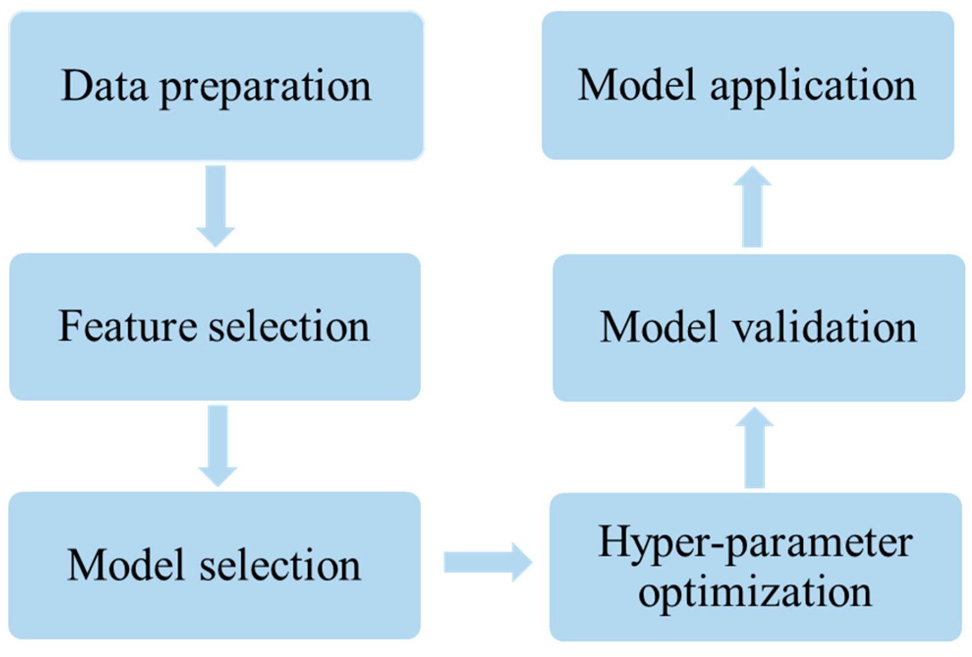
2.1. The Flowchart of Materials Data Mining
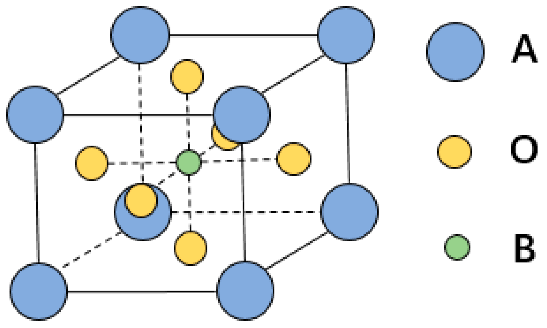
2.2. Data Preparation
2.3. Machine Learning Methods
2.3.1. Gradient Boosting Regression (GBR)
2.3.2. Decision Tree Regression (DTR)
2.3.3. Random Forest Regression (RFR)
2.3.4. Support Vector Regression (SVR)
2.4. Computational Software
3. Results and Discussion
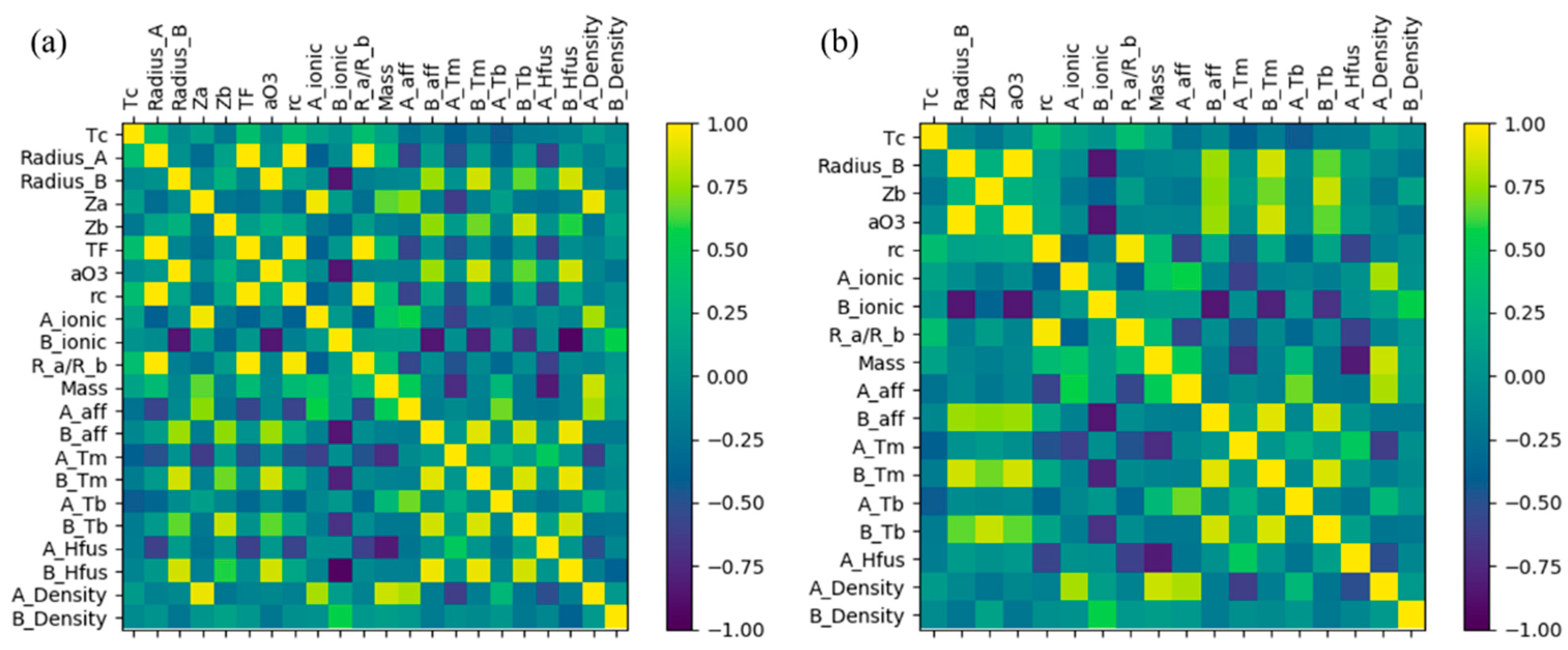
3.1. Feature Selection
3.2. Model Selection
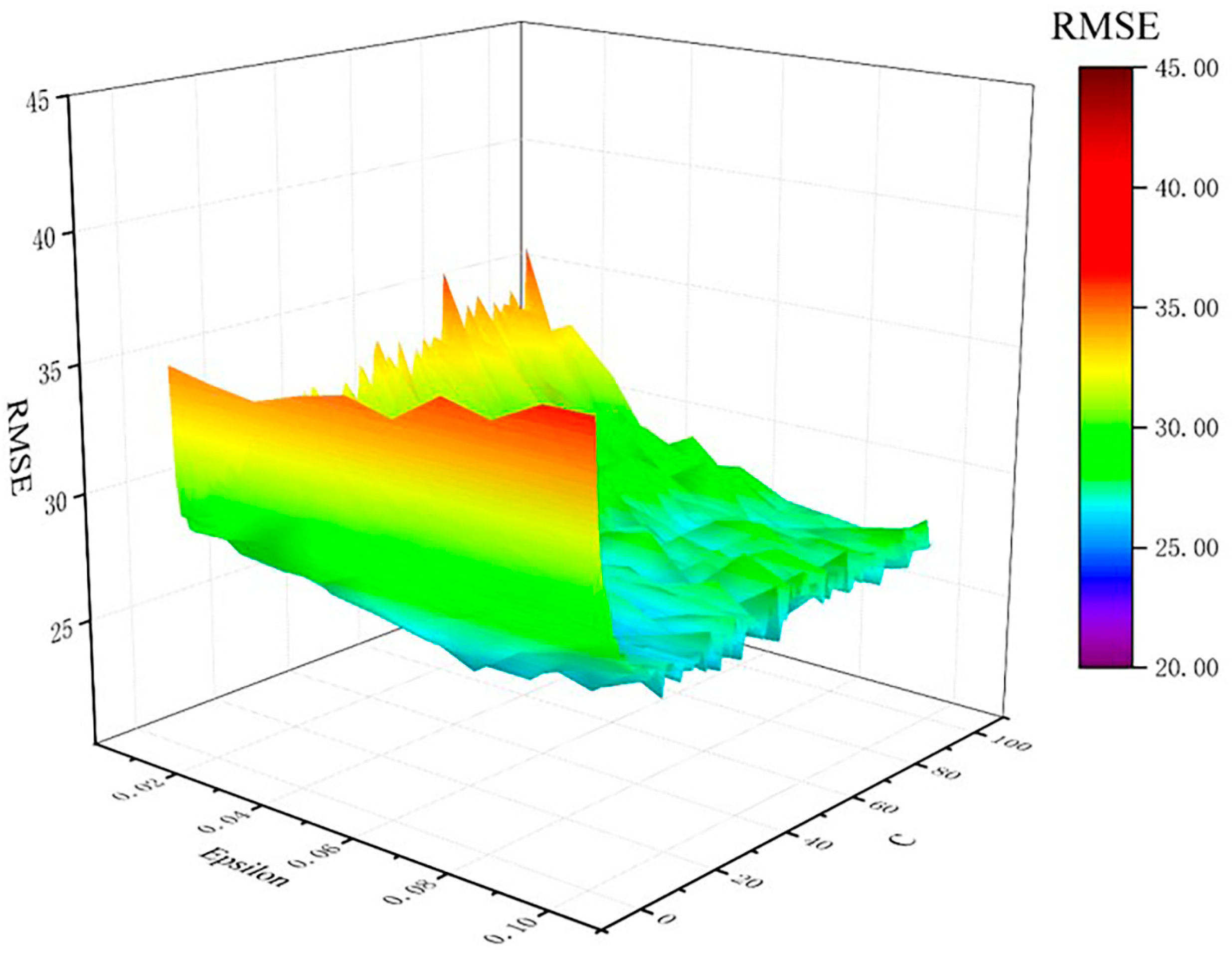
3.3. Hyper-Parameter Optimization
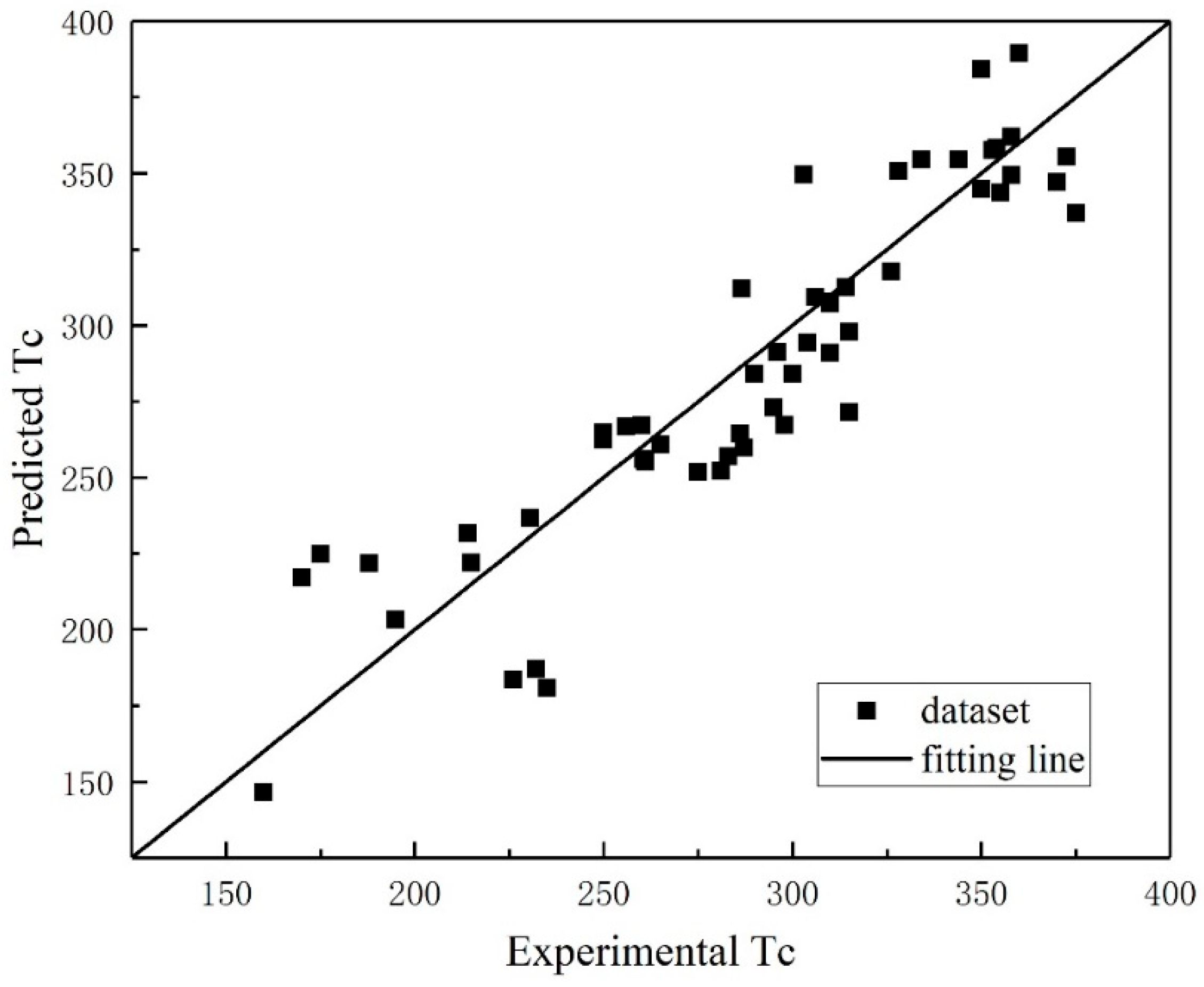
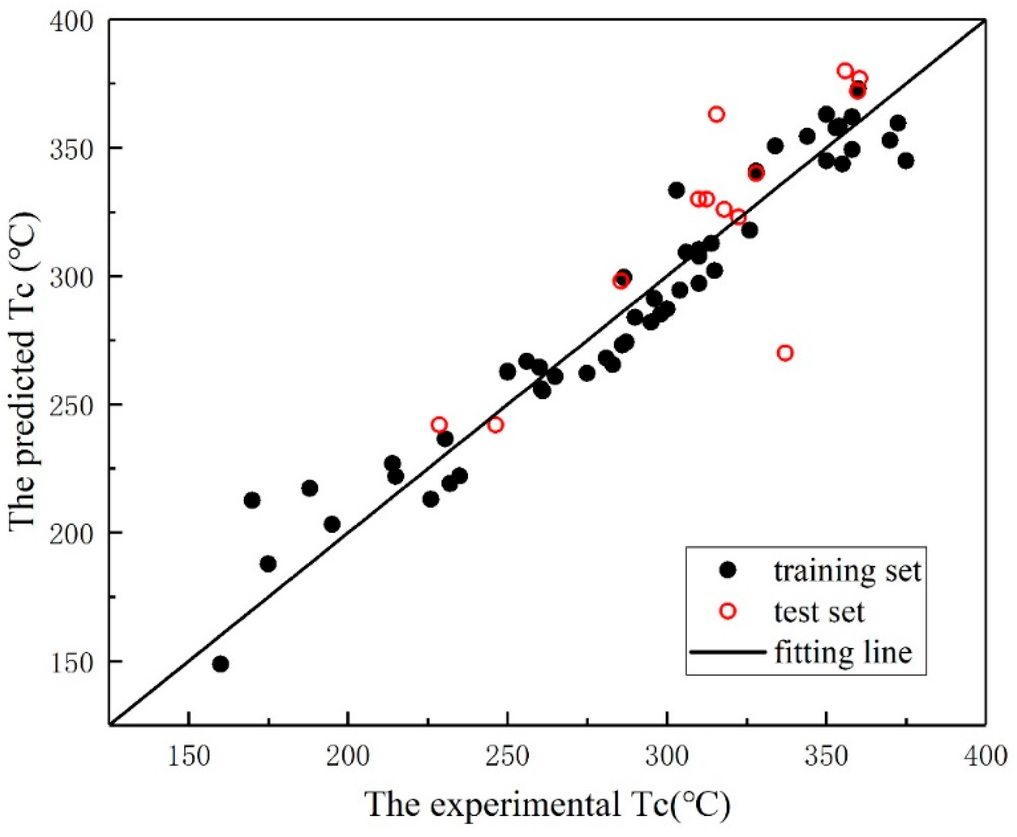
3.4. Model Validation
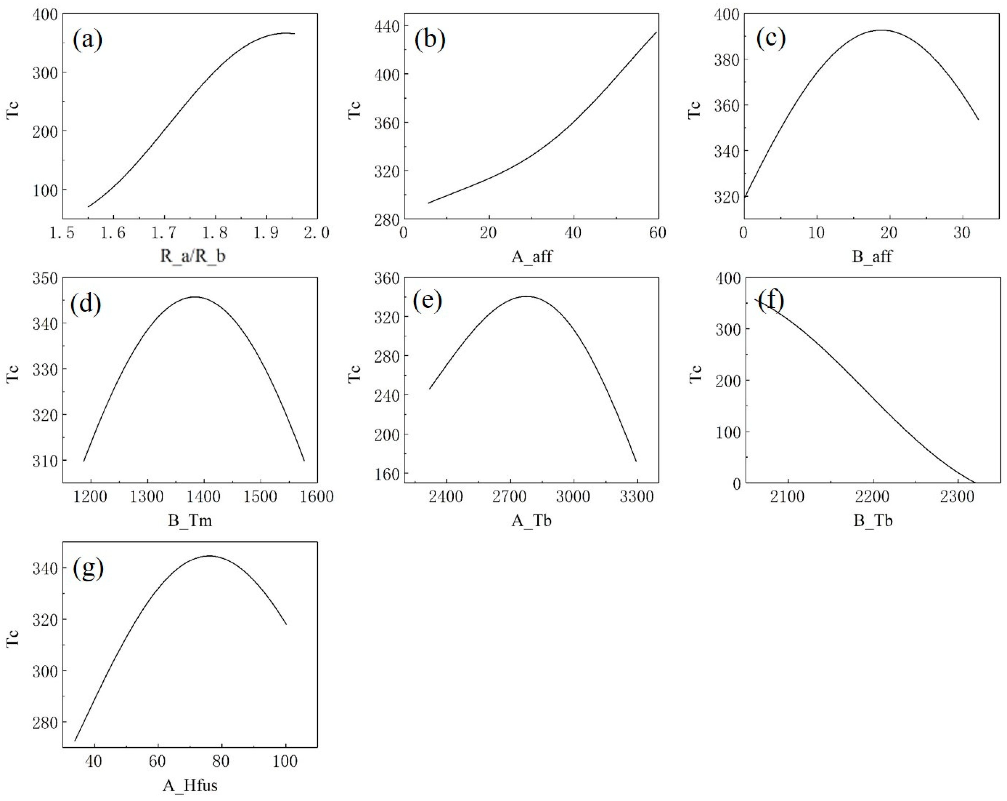
3.5. Sensitivity Analysis
3.6. Model Application
3.6.1. High-Throughput Screening of New Lanthanum Manganite Perovskites
- (1)
- The A site is doped with no more than two different doping ions, while the B site is doped with no more than one doping ion.
- (2)
- The A site compositional configuration follows a ternary doping scheme:
- Primary occupant: La with stoichiometric ratios spanning 0.5–1.0 in 0.02 increments.
- Secondary dopant: Sr, Ag, Ca, Pb, or Ba allocated within the 0.0–0.5 range (0.02 step resolution).
- Tertiary constituent: Nd, Ba, Ag, Ca, or Dy occupying residual stoichiometric fractions.
- (3)
- The B-site doping architecture adopts a two-component system:
- Primary constituent: Mn with stoichiometric fractions ranging 0.9–1.0 in 0.02 incremental steps.
- Secondary dopant: Fe or Cr occupying the complementary stoichiometric proportion.
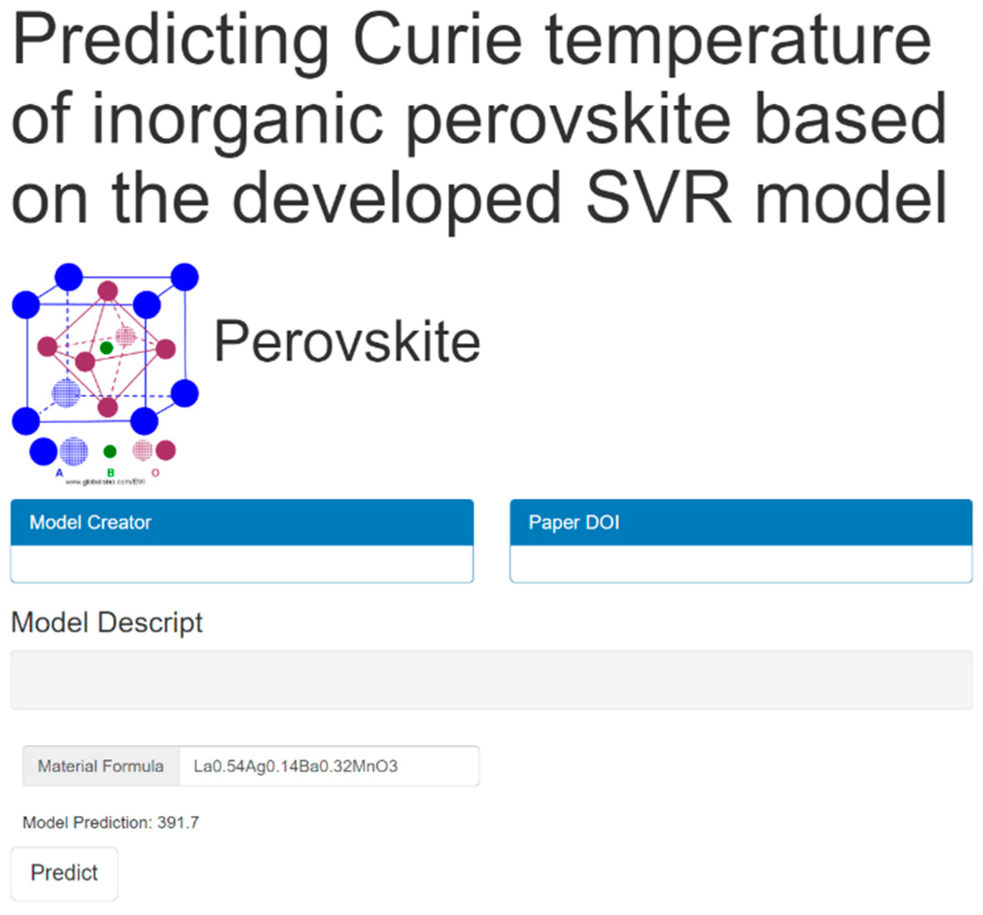
3.6.2. Online Web Server Accessible in Public
4. Conclusions
Supplementary Materials
Author Contributions
Funding
Institutional Review Board Statement
Informed Consent Statement
Data Availability Statement
Conflicts of Interest
References
- Yan, R.; Zou, Y.; Du, C.; Yu, H.; Jiang, J.; Cao, J.; Yu, G.; Dong, W.; Peng, H.; Yang, Y.; et al. Research progress of polarized perovskite type ferroelectric materials for photocatalytic hydrogen production. J. Energy Chem. 2025, 107, 87–102. [Google Scholar] [CrossRef]
- Li, Q.; Zheng, Y.; Wang, H.; Liu, X.; Lin, M.; Sui, X.; Leng, X.; Liu, D.; Wei, Z.; Song, M.; et al. Graphene-polymer reinforcement of perovskite lattices for durable solar cells. Science 2025, 387, 1069–1077. [Google Scholar] [CrossRef]
- Xu, H.; Guo, W.; Liu, Y.; Ma, Y.; Fan, Q.; Tang, L.; Li, W.; Ni, H.; Luo, J.; Sun, Z. Customizing Room-Temperature Perovskite Ferroelectrics toward the Multichannel Domain Manipulation. Angew. Chem. Int. Ed. 2025, e202501238. [Google Scholar] [CrossRef]
- Liu, Z.; Zhang, S.; Wang, X.; Ye, X.; Qin, S.; Shen, X.; Lu, D.; Dai, J.; Cao, Y.; Chen, K.; et al. Realization of a Half Metal with a Record-High Curie Temperature in Perovskite Oxides. Adv. Mater. 2022, 34, e2200626. [Google Scholar] [CrossRef] [PubMed]
- Yao, Y.; Jiang, H.; Peng, Y.; Zhang, X.; Chen, S.; Liu, X.; Luo, J. High-Curie Temperature Multilayered Hybrid Double Perovskite Photoferroelectrics Induced by Aromatic Cation Alloying. J. Am. Chem. Soc 2021, 143, 15900–15906. [Google Scholar] [CrossRef]
- Sun, K.; Liu, S.; Gao, Y.; Du, H.; Cheng, D.; Wang, Z. Output power prediction of stratospheric airship solar array based on surrogate model under global wind field. Chin. J. Aeronaut. 2025, 38, 103244. [Google Scholar] [CrossRef]
- Li, K.; Zhu, Y.; Chang, X.; Zhou, M.; Yu, X.; Zhao, X.; Wang, T.; Cai, Z.; Zhu, X.; Wang, H.; et al. Self-Induced Bi-interfacial Modification via Fluoropyridinic Acid For High-Performance Inverted Perovskite Solar Cells. Adv. Energy Mater. 2024, 15, 613. [Google Scholar] [CrossRef]
- Yang, Y.; Xiang, H.; Zhao, H.; Stroppa, A.; Zhang, J.; Cao, S.; Íñiguez, J.; Bellaiche, L.; Ren, W. Improper ferroelectricity at antiferromagnetic domain walls of perovskite oxides. Phys. Rev. B 2017, 96, 104431. [Google Scholar] [CrossRef]
- Abassi, M.; Dhahri, N.; Dhahri, J.; Hlil, E.K. Structural and large magnetocaloric properties of La0.67-xYxBa0.23Ca0.1MnO3 perovskites (0< = × < = 0.15). Physica B Condens. Matter 2014, 449, 138–143. [Google Scholar] [CrossRef]
- Anwar, M.S.; Ahmed, F.; Koo, B.H. Structural distortion effect on the magnetization and magnetocaloric effect in Pr modified La0.65Sr0.35MnO3 manganite. J. Alloys Compd. 2014, 617, 893–898. [Google Scholar] [CrossRef]
- Anwar, M.S.; Ahmed, F.; Koo, B.H. Influence of Ce addition on the structural, magnetic, and magnetocaloric properties in La0.7-xCexSr0.3MnO3 (0 < = × < = 0.3) ceramic compound. Ceram. Int. 2015, 41, 5821–5829. [Google Scholar] [CrossRef]
- Arayedh, B.; Kallel, S.; Kallel, N.; Peña, O. Influence of non-magnetic and magnetic ions on the MagnetoCaloric properties of La0.7Sr0.3Mn0.9M0.1O3 doped in the Mn sites by M = Cr, Sn, Ti. J. Magn. Magn. Mater. 2014, 361, 68–73. [Google Scholar] [CrossRef]
- Chau, N.; Nhat, H.N.; Luong, N.H.; Minh, D.L.; Tho, N.D.; Chau, N.N. Structure, magnetic, magnetocaloric and magnetoresistance properties of La1-xPbxMnO3 perovskite. Physica B Condens. Matter 2003, 327, 270–278. [Google Scholar] [CrossRef]
- Debnath, J.C.; Zeng, R.; Kim, J.H.; Dou, S.X. Large magnetic entropy change near room temperature in La0.7(Ca0.27Ag0.03)MnO3 perovskite. J. Alloys Compd. 2011, 509, 3699–3704. [Google Scholar] [CrossRef]
- Dhahri, J.; Dhahri, A.; Oummezzine, M.; Hlil, E.K. Effect of substitution of Fe for Mn on the structural, magnetic properties and magnetocaloric effect of LaNdSrCaMnO3. J. Magn. Magn. Mater. 2015, 378, 353–357. [Google Scholar] [CrossRef]
- Ghodhbane, S.; Tka, E.; Dhahri, J.; Hlil, E.K. A large magnetic entropy change near room temperature in La0.8Ba0.1Ca0.1Mn0.97Fe0.03O3 perovskite. J. Alloys Compd. 2014, 600, 172–177. [Google Scholar] [CrossRef]
- Kallel, N.; Kallel, S.; Hagaza, A.; Oumezzine, M. Magnetocaloric properties in the Cr-doped La0.7Sr0.3MnO3 manganites. Physica B Condens. Matter 2009, 404, 285–288. [Google Scholar] [CrossRef]
- Koubaa, M.; Koubaa, W.C.-R.; Cheikhrouhou, A. Magnetocaloric effect and magnetic properties of La0.75Ba0.1M0.15MnO3 (M = Na, Ag and K) perovskite manganites. J. Alloys Compd. 2009, 479, 65–70. [Google Scholar] [CrossRef]
- Koubaa, W.C.-R.; Koubaa, M.; Cheikhrouhou, A. Structural, magnetotransport, and magnetocaloric properties of La0.7Sr0.3-xAgxMnO3 perovskite manganites. J. Alloys Compd. 2008, 453, 42–48. [Google Scholar] [CrossRef]
- Li, B.H.; Xian-Yu, W.X.; Wan, X.; Zhang, J.; Shen, B.G. Colossal magnetoresistance effects and magnetic properties of La0.7Sr0.3MxMn1−xO3(M = Cr,Fe). Acta Phys. Sin. 2000, 49, 1366–1370. [Google Scholar]
- Phan, M.H.; Tian, S.B.; Hoang, D.Q.; Yu, S.C.; Nguyen, C.; Ulyanov, A.N. Large magnetic-entropy change above 300 K in CMR materials. J. Magn. Magn. Mater. 2003, 258, 309–311. [Google Scholar] [CrossRef]
- Sankarrajan, S.; Sakthipandi, K.; Manivasakan, P.; Thyagarajan, K.; Rajendran, V. On-line phase transition in La1-xSrxMnO3 (0.28 < = x < = 0.36) perovskites through ultrasonic studies. Phase Transit. 2011, 84, 657–672. [Google Scholar] [CrossRef]
- Zhang, D.; Du, Y. Relation between structure and Curie-temperature of peroviskite with colossal magnetoresistance effect. J. Funct. Mater. 2002, 33, 495–496, 499. [Google Scholar]
- Zhao, J.; Li, L.; Wang, G. Magnetocaloric Properties in (La0.57Dy0.1)Sr0.33MnO3 Poly-crystalline Nanoparticles. Rare Met. Mater. Eng. 2009, 38, 1707–1710. [Google Scholar]
- James Speight, P.D. Lange’s Handbook of Chemistry, 16th ed.; McGraw-Hill Education: New York, NY, USA, 2005. [Google Scholar]
- Friedman, J.H. Greedy function approximation: A gradient boosting machine. Ann. Math. Stat. 2001, 29, 1189–1232. [Google Scholar] [CrossRef]
- Friedman, J.H. Stochastic gradient boosting. Comput. Stat. Data Anal. 2002, 38, 367–378. [Google Scholar] [CrossRef]
- Wu, T.; Wang, J. Global discovery of stable and non-toxic hybrid organic-inorganic perovskites for photovoltaic systems by combining machine learning method with first principle calculations. Nano Energy 2019, 66, 104070. [Google Scholar] [CrossRef]
- Witman, M.; Ling, S.; Grant, D.M.; Walker, G.S.; Agarwal, S.; Stavila, V.; Allendorf, M.D. Extracting an Empirical Intermetallic Hydride Design Principle from Limited Data via Interpretable Machine Learning. J. Phys. Chem. Lett. 2020, 11, 40–47. [Google Scholar] [CrossRef]
- Im, J.; Lee, S.; Ko, T.-W.; Kim, H.W.; Hyon, Y.; Chang, H. Identifying Pb-free perovskites for solar cells by machine learning. npj Comput. Mater. 2019, 5, 37. [Google Scholar] [CrossRef]
- Breiman, L. Classification and Regression Trees; Routledge: London, UK, 2017. [Google Scholar]
- Pilania, G.; Liu, X.-Y.; Wang, Z. Data-enabled structure–property mappings for lanthanide-activated inorganic scintillators. J. Mater. Sci. 2019, 54, 8361–8380. [Google Scholar] [CrossRef]
- Meredig, B.; Agrawal, A.; Kirklin, S.; Saal, J.E.; Doak, J.W.; Thompson, A.; Zhang, K.; Choudhary, A.; Wolverton, C. Combinatorial screening for new materials in unconstrained composition space with machine learning. Phys. Rev. B 2014, 89, 094104. [Google Scholar] [CrossRef]
- Zeng, Y.; Li, Q.; Bai, K. Prediction of interstitial diffusion activation energies of nitrogen, oxygen, boron and carbon in bcc, fcc, and hcp metals using machine learning. Comput. Mater. Sci. 2018, 144, 232–247. [Google Scholar] [CrossRef]
- Breiman, L. Random forests. Mach. Learn. 2001, 45, 5–32. [Google Scholar] [CrossRef]
- Stanev, V.; Oses, C.; Kusne, A.G.; Rodriguez, E.; Paglione, J.; Curtarolo, S.; Takeuchi, I. Machine learning modeling of superconducting critical temperature. npj Comput. Mater. 2018, 4, 29. [Google Scholar] [CrossRef]
- Harikrishna, S.; Weining, R.; Alessandro, T.; Haibo, M. Toward Predicting Efficiency of Organic Solar Cells via Machine Learning and Improved Descriptors. Adv. Energy Mater. 2018, 8, 1801032. [Google Scholar] [CrossRef]
- Zhu, Q.; Xu, P.; Ji, X.; Shao, M.; Duan, Z.; Lu, W. Discovery and verification of two-dimensional organic–inorganic hybrid perovskites via diagrammatic machine learning model. Mater. Des. 2024, 238, 112642. [Google Scholar] [CrossRef]
- Vapnik, V.N. The Nature of Statistical Learning Theory; Springer: New York, NY, USA, 2000. [Google Scholar]
- Möller, J.J.; Körner, W.; Krugel, G.; Urban, D.F.; Elsässer, C. Compositional optimization of hard-magnetic phases with machine-learning models. Acta Mater. 2018, 153, 53–61. [Google Scholar] [CrossRef]
- Balachandran, P.V.; Kowalski, B.; Sehirlioglu, A.; Lookman, T. Experimental search for high-temperature ferroelectric perovskites guided by two-step machine learning. Nat. Commun. 2018, 9, 1668. [Google Scholar] [CrossRef]
- Che, H.; Lu, T.; Cai, S.; Li, M.; Lu, W. Inverse Design of Low-Resistivity Ternary Gold Alloys via Interpretable Machine Learning and Proactive Search Progress. Materials 2024, 17, 3614. [Google Scholar] [CrossRef]
- Zhang, Q.; Chang, D.; Zhai, X.; Lu, W. OCPMDM: Online computation platform for materials data mining. Chemom. Intell. Lab. Syst. 2018, 177, 26–34. [Google Scholar] [CrossRef]
- Chang, D.; Xu, P.; Ji, X.; Li, M.; Lu, W. Application of Online Computational Platform of Materials Data Mining (OCPMDM) in Search for ABO3 Perovskites with Multi-Properties. Sci. Adv. Mater. 2023, 15, 1014–1025. [Google Scholar] [CrossRef]
- Tao, Q.; Xu, P.; Li, M.; Lu, W. Machine learning for perovskite materials design and discovery. npj. Comput. Mater. 2021, 7, 23. [Google Scholar] [CrossRef]
- Browning, N.J.; Ramakrishnan, R.; von Lilienfeld, O.A.; Roethlisberger, U. Genetic Optimization of Training Sets for Improved Machine Learning Models of Molecular Properties. J. Phys. Chem. Lett. 2017, 8, 1351–1359. [Google Scholar] [CrossRef]
- Wang, H. Forward Regression for Ultra-High Dimensional Variable Screening. J. Am. Stat. Assoc. 2009, 104, 1512–1524. [Google Scholar] [CrossRef]
- Ramprasad, R.; Batra, R.; Pilania, G.; Mannodi-Kanakkithodi, A.; Kim, C. Machine learning in materials informatics: Recent applications and prospects. npj Comput. Mater. 2017, 3, 54. [Google Scholar] [CrossRef]
- Butler, K.T.; Davies, D.W.; Cartwright, H.; Isayev, O.; Walsh, A. Machine learning for molecular and materials science. Nature 2018, 559, 547–555. [Google Scholar] [CrossRef]
- Taboada-Moreno, C.A.; Sánchez-De Jesús, F.; Pedro-García, F.; Cortés-Escobedo, C.A.; Betancourt-Cantera, J.A.; Ramírez-Cardona, M.; Bolarín-Miró, A.M. Large magnetocaloric effect near to room temperature in Sr doped La0.7Ca0.3MnO3. J. Magn. Magn. Mater. 2020, 496, 165887. [Google Scholar] [CrossRef]
- Shreekala, R.; Rajeswari, M.; Srivastava, R.C.; Ghosh, K.; Eom, C.B. Ferromagnetism at room temperature in La0.8Ca0.2MnO3 thin films. Appl. Phys. Lett. 1999, 74, 1886–1888. [Google Scholar] [CrossRef]
- Schiffer, P.; Ramirez, A.P.; Bao, W.; Cheong, S.W. Low Temperature Magnetoresistance and the Magnetic Phase Diagram of La1−xCaxMnO3. Phys. Rev. Lett. 1995, 75, 3336–3339. [Google Scholar] [CrossRef]
- Prellier, W.; Rajeswari, M.; Venkatesan, T.; Greene, R.L. Effects of annealing and strain on La1−xCaxMnO3 thin films: A phase diagram in the ferromagnetic region. Appl. Phys. Lett. 1999, 75, 1446–1448. [Google Scholar] [CrossRef]
- Fontcuberta, J.; Laukhin, V.; Obradors, X. Local disorder effects on the pressure dependence of the metal-insulator transition in manganese perovskites. Appl. Phys. Lett. 1998, 72, 2607–2609. [Google Scholar] [CrossRef]

| No. | Feature Name | Feature Description |
|---|---|---|
| 01 | Radius_A | atomic radius of the A position |
| 02 | Radius_B | atomic radius of the B position |
| 03 | Ea | electronegativity of the A position |
| 04 | Eb | electronegativity of the B position |
| 05 | TF | tolerance factor |
| 06 | αO3 | unit cell lattice edge |
| 07 | rc | critical radius |
| 08 | Za | ionization potential of the A position |
| 09 | Zb | ionization potential of the B position |
| 10 | R_a/R_b | ratio of the atomic radius of the A and B positions |
| 11 | Mass | molecular mass |
| 12 | A_aff | electron affinity of the A position |
| 13 | B_aff | electron affinity of the B position |
| 14 | A_Tm | melting point of the A position |
| 15 | B_Tm | melting point of the B position |
| 16 | A_Tb | normal boiling point of the A position |
| 17 | B_Tb | normal boiling point of the B position |
| 18 | A_Hfus | enthalpy of fusion at the melting point of the A position |
| 19 | B_Hfus | enthalpy of fusion at the melting point of the B position |
| 20 | D_A | density of the A position |
| 21 | D_B | density of the B position |
| Algorithm | RMSE (K) | R | The Number of Selected Features | The Selected Features |
|---|---|---|---|---|
| Genetic Algorithm | 38.72 | 0.7658 | 7 | Zb, aO3, A_ionic, R_a/R_b, A_aff, B_aff, A_Tb |
| Forward Regression | 26.51 | 0.8849 | 7 | R_a/R_b, A_aff, B_aff, B_Tm, A_Tb, B_Tb, A_Hfus |
| Backward Regression | 28.29 | 0.8632 | 4 | R_a/R_b, A_aff, A_Tb, B_Tb |
| Algorithm | R | RMSE (K) | MRE |
|---|---|---|---|
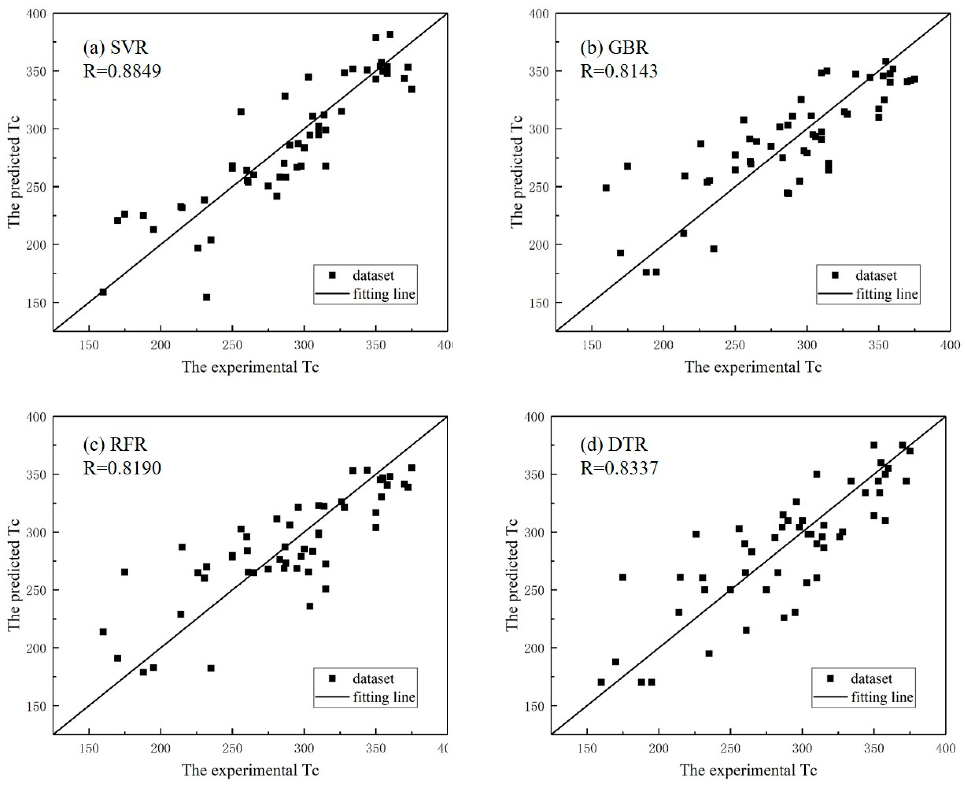
| SVR | 0.8849 | 26.50 | 0.0790 |
| GBR | 0.8143 | 32.19 | 0.1011 |
| RFR | 0.8190 | 31.82 | 0.0972 |
| DTR | 0.8337 | 31.29 | 0.0937 |
| Algorithm | R | RMSE (K) | MAE (K) | MRE |
|---|---|---|---|---|
| SVR | 0.9111 | 23.82 | 18.94 | 0.0720 |
| Algorithm | R | RMSE (K) | MAE (K) | MRE |
|---|---|---|---|---|
| SVR | 0.8385 | 26.36 | 19.67 | 0.0623 |
Disclaimer/Publisher’s Note: The statements, opinions and data contained in all publications are solely those of the individual author(s) and contributor(s) and not of MDPI and/or the editor(s). MDPI and/or the editor(s) disclaim responsibility for any injury to people or property resulting from any ideas, methods, instructions or products referred to in the content. |
© 2025 by the authors. Licensee MDPI, Basel, Switzerland. This article is an open access article distributed under the terms and conditions of the Creative Commons Attribution (CC BY) license (https://creativecommons.org/licenses/by/4.0/).
Share and Cite
Tian, L.; Wang, W.; Ji, X.; Xu, Z.; Zhou, W.; Lu, W. Data-Mining-Aided-Material Design of Doped LaMnO3 Perovskites with Higher Curie Temperature. Materials 2025, 18, 2437. https://doi.org/10.3390/ma18112437
Tian L, Wang W, Ji X, Xu Z, Zhou W, Lu W. Data-Mining-Aided-Material Design of Doped LaMnO3 Perovskites with Higher Curie Temperature. Materials. 2025; 18(11):2437. https://doi.org/10.3390/ma18112437
Chicago/Turabian StyleTian, Lumin, Wentan Wang, Xiaobo Ji, Zhibin Xu, Wenyan Zhou, and Wencong Lu. 2025. "Data-Mining-Aided-Material Design of Doped LaMnO3 Perovskites with Higher Curie Temperature" Materials 18, no. 11: 2437. https://doi.org/10.3390/ma18112437
APA StyleTian, L., Wang, W., Ji, X., Xu, Z., Zhou, W., & Lu, W. (2025). Data-Mining-Aided-Material Design of Doped LaMnO3 Perovskites with Higher Curie Temperature. Materials, 18(11), 2437. https://doi.org/10.3390/ma18112437