Abstract
This study addresses the challenge of optimizing seal structure design through a novel two-stage interpretable optimization framework. Focusing on O-ring waterproof performance under hyperelastic material behavior, this study proposes a double-layer optimization method integrating explainable machine learning with hierarchical clustering algorithms. The key innovation lies in employing modified hierarchical clustering to categorize design parameters into two interpretable groups: bolt preload and groove depth. This clustering enables dimensionality reduction while maintaining the physical interpretability of critical parameters. In the first layer, systematic parameter screening and optimization are applied to the preload variable to reduce the database, with six remaining data points that constitute one-seventh of the original data. The second layer subsequently refines configurations using E-TOPSIS (Entropy Weight—Technique for Order Preference by Similarity to Ideal Solution) optimization. All evaluations are performed through FEA (finite element analysis) considering nonlinear material responses. The optimal design is a groove depth of 0.8 mm and a preload of 80 N. The experimental validation demonstrates that this method efficiently identifies optimal designs meeting IPX8 waterproof requirements, with zero leakage observed in both O-ring surfaces and motor interiors. The proposed methodology provides physically meaningful design guidelines.
1. Introduction
Sealing structures with hyperelastic material are widely used in the automobile industry (Figure 1a), aviation industry (Figure 1b), and aerospace industry (Figure 1c) in sealing parts in various fields. For space stations, one of the main goals of deep-space exploration is to ensure that astronauts have a space station environment that is suitable for work and life and stops air from leaking out after docking. Sealing structures are also used in many products, such as air-pumping systems [1], the radial shaft sealing rings of production robots [2], and reciprocating sealing in marine applications [3].
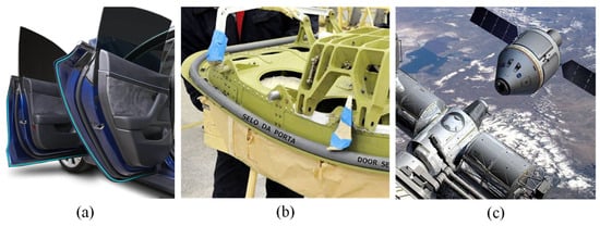
Figure 1.
The application of sealing structures with rubber seals: (a) Automobile door sealing strip. (b) Aircraft door sealing strip. (c) Manned capsule docking seal structure [4].
The CAE method, theoretical calculation, and experimental tests are the main methods of hyperelastic material research in sealing structure design. Research in this area can be summarized through the following aspects.
In the field of composite seal design, Han Yan proposed a machine learning framework method combining finite elements and artificial intelligence for predicting the sealing and mechanical properties of fabric–rubber composites [5]. Yifeng Dong, based on the microchannel model, studied in detail the mechanical behavior and leakage characteristics of fabric–rubber composites in aircraft doors and established an explicit expression for the gas leakage rate at the contact interface of fabric–rubber composites. Through dimensional analysis, finite element analysis, and computational fluid dynamics (CFD) methods, an explicit non-dimensional function of the gas leakage rate at the contact interface of rubber seals was proposed [6]. Xiaoyao Xu studied the mechanical properties of non-orthogonal mesh fabric-reinforced rubber composites and their composite fabric rubber seals. The macro behavior of complex fabric rubber seals was studied through experiments and numerical simulations [7].
In the field of optimization of sealing performance and failure analysis, Jin Guo used the finite element software product to study the sealing characteristics of a non-standard seal and designed and optimized the structure of the non-standard seal. A new type D seal, composed of rubber and EPDM foam, was designed. The design scheme was tested and the simulation results verified the accuracy of the calculation [8]. Ganlin Cheng found that the main reason for seal failure of the ACGT-HP combined rod seal of an aircraft actuator is that various inappropriate coupling factors aggravate seal wear, resulting in a rapid reduction in contact stress and seal failure [9]. Yongjie Zhang’s research is based on experimental and numerical simulations analyzing helicopter landing pad friction faults. Three kinds of composite sealing structures were introduced to enhance the sealing performance of the buffer column, and the inherent defects of the original O-ring structure were repaired, providing an optimal contact pressure range for optimized seals [10]. Jia-Bin Wu tested the physical stress relaxation properties of nitrile butadiene rubber at a low temperature of 4 °C. The finite element numerical model of the O-ring seal structure for a deep-sea hydraulic system was established. It was concluded that the reliability of the O-ring sealing structure in a deep-sea hydraulic system continues to decline, and increasing the initial compression of the O-ring can effectively improve its sealing reliability [11]. Mei Yang et al. designed an O-ring with a skeleton seal by numerical analysis for the storage tank gate of a cutter-changing robot in large-diameter shield machines, enhancing its applicability [12]. Zhibin Zhang et al. analyzed the extrusion–occlusion dynamic failure of O-rings based on floating bushes in water hydraulic pumps [13].
In the field of mechanics behavior and contact pressure of O-rings, Yangtao Xing proposed an analytical method for investigating the contact characteristics of rubber shaft seals under dynamic eccentricity. The method improves the calculation accuracy of rubber shaft seal contact under dynamic eccentricity [14]. Zhi Chen et al. used the numerical simulation method to simulate the O-ring and concluded that excessive compression is not conducive to the sealing performance of the mechanical seal. The partial compression of the O-ring directly affects the deformation of the end face of the flexible ring [15]. Hyung-Kyu Kim used finite element analysis, experiments, and traditional theory to study the contact stress for a compressed and laterally one-side restrained O-ring [16]. Zhou et al. used the finite element analysis method and investigated the stress and contact pressure on rubber sealing O-rings under different boundary conditions [17]. Karaszkiewicz examined the geometry and contact pressure of an O-ring mounted in a seal groove [18]. Eugenio Dragoni and Antonio Strozzi provided a theoretical analysis of an unpressurized elastomeric O-ring seal inserted into a rectangular groove to describe mechanical behavior [19]. Isaac Fried and Arthur R. Johnson focused on computing the nonlinear deformation of axisymmetric solid rubber [20]. A.F. George, A. Strozzi, and J.I. Rich compared computer predictions and experimental results to investigate stress fields in a compressed unconstrained elastomeric O-ring seal [21]. Shukla and Nigam proposed a numerical–experimental analysis of the contact stress problem using full-field photoelastic data [22].
In the field of rubber sealing materials in hydrogen environments. Chilou Zhou systematically elaborated the mechanism of hydrogen-induced bubble breakage in rubber, taking into account the compression state and field performance of rubber O-rings [23,24]. Clara Clute studied five different fillers and curing agents for nitrile butadiene rubber (NBR) vulcanizates to understand the impact of additives on the performance of rubber grades suitable for high-pressure hydrogen infrastructure seals [25]. Junichiro Yamabe et al. examined the failure behavior of rubber O-rings exposed to high-pressure hydrogen gas, revealing failure modes under extreme conditions [26].
In the field of durability studies, Christopher Porter et al. critically examined the shelf life of nitrile rubber O-rings used in aerospace sealing applications and found that various physical properties of the O-ring increased with the increase in aging time [27]. Morrell P. R., M. Patel, and A. R. Skinner investigated the accelerated thermal aging of nitrile rubber O-rings, oxidation crossing leads to hardening and brittleness of the material, providing important information about material lifespan [28].
TOPSIS (Technique for Order Preference by Similarity to an Ideal Solution) has been used as a reliable tool in many fields, such as energy supplier selection [29], novel materials with anti-aging functionality [30], energy dissipation devices [31], hydrokinetic energy harvesters [32], electric vehicles [33], automotive styling design evaluation [34], multi-energy complementary heating systems [35], high-strength concrete [36], energy storage power station [37], metal inert gas welding process [38], etc. However, some studies rarely mention the application of TOPSIS algorithms in sealing structure design optimization. Finite element results under different working conditions are established to study the sealing characteristics of the O-ring sealing structure. The simulation results show different trends. Therefore, this study introduced TOPSIS to find the best design. The simulation model also provides the contour plot and database for ML and TOPSIS for optimization.
Explainable artificial intelligence (XAI) emerges as a pivotal enabler in the evolutionary trajectory from Industry 4.0 to Industry 5.0 paradigms, functioning as a foundational mechanism for demystifying algorithmic decision-making processes through enhanced interpretability, thereby mitigating epistemic uncertainties and augmenting stakeholder trust in AI-driven systems while aligning with techno ethical imperatives of transparency and accountability [39,40,41]. Explainable artificial intelligence helps engineers quickly locate the optimal geometric configuration and loading method by revealing the causal relationship between key parameters and sealing performance in the optimized design of sealing structures, significantly shortening the traditional trial-and-error cycle [42,43].
Hierarchical clustering is an unsupervised learning technique that groups data points into nested clusters using a tree-like structure (dendrogram), either merging similar clusters (agglomerative) or dividing dissimilar ones (divisive). Compared with common algorithms such as K-means and DBSCAN [44,45], it dynamically reveals multi-scale relationships without requiring prior specification of cluster count. Machine learning hierarchical clusters classify the database provided by the FEA results.
2. Models
2.1. Physical Model
Figure 2 shows a 3D motor model with the O-ring, base, and shell. There are five contact surfaces and three of them are around the O-ring. Contact surfaces 1 to 3 are the main working contact surfaces of the rubber seal. When the contact pressure of these three contact surfaces is larger than the ambient pressure (e.g., water pressure), the sealing structure works.
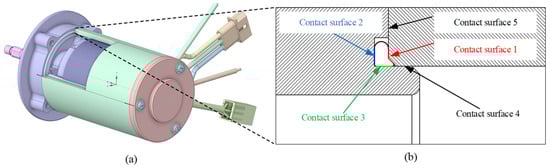
Figure 2.
Motor model with rubber seal: (a) O-ring position and (b) contact surfaces.
Another key physical quantity that is considered is the von Mises stress of the O-ring, which determines whether the rubber material works normally. If the stress is larger than the yield limit of the rubber material, then the O-ring will fail [46,47]. Formula (1) describes von Mises stress σ, where are the principal stresses.
The input parameters are H and preload: H is the groove depth that varies from 0.6 to 0.9 mm in Figure 3 with the diameter of the O-ring being 1.5 mm. The preload of each bolt varies from 30 N to 80 N. The FEA model is established and the mechanical performance is simulated. The FEA results include a lot of physical quantity. This paper considers the main physical quantities, which are contact area, contact pressure, and O-ring stress.
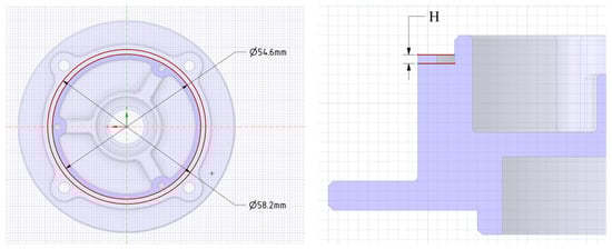
Figure 3.
Groove dimension parameters.
2.2. Numerical Model
Contact, geometric, and material nonlinearities are the main characteristics of rubber materials, and the Poisson ratio is close to 0.5 [48]. In this study, the Mooney–Rivlin model describes the hyperelastic characteristic [49,50]. The strain energy density function ψ is as follows:
J is the Jacobian, d is the material incompressibility parameter, and C10 and C01 are material constants; these material data are provided in the ANSYS material database, which is ANSYS Granta Selector 2023 R2 software [51,52]. .
In this study, the material of the motor shell is structure steel, the base and cover are aluminum alloy, and the material properties are listed in Table 1. Five contact surfaces are listed in Table 2 with the friction coefficient.

Table 1.
Material properties.
Table 2.
Friction coefficient of different contact surfaces.
Bolt preload locked the shell, base, and cover in the axial direction in Figure 4a, which makes the O-ring seal work when it compresses. The bolt hole is fixed in Figure 4b. In order to speed up the simulation and shorten the calculation time, the model used a beam connection. Beam connections ignore the geometry of bolts, washers, and nuts, which can speed up the analysis and save simulation time. In this study, the ‘Stabilization’ option and ‘Large Deflection’ option are considered.
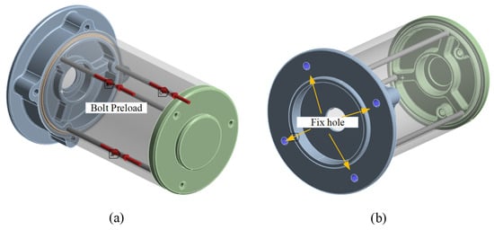
Figure 4.
Boundary conditions: (a) bolt preload direction and (b) fix bolt hole.
There are 3 contact pairs around the O-ring. In the ANSYS mechanical software, each contact pairs have 2 contact surfaces which are named contact surface and target surface. The contact surface cannot penetrate the target surface. The O-ring surface is set as the contact surface, and the shell and groove surface are set as the target surfaces. The difference between the target surface and the contact surface is shown in Figure 5.
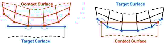
Figure 5.
Target surface and contact surface [53].
2.3. Grid Independence Verification
In order to save resources, a grid independence test was carried out to find the appropriate element number while considering the accuracy and reliability of computing results and saving computing time. The coarse mesh (element number 224243), medium mesh (element number 372294), and fine mesh (element number 627654) are listed in Table 3 and Figure 6, respectively. These models consume about 1 h, 3 h, and 10 h through ANSYS workbench 2023 R2. Comparing the simulation results, the medium mesh results are close to that of the fine mesh. The fine mesh model costs more than 10 h, which can lead to the established database being time too long, and it increases the risk of computer crashes. Thus, element 372294 was selected, and the element size was applied to the other models in this research to establish a database for ML.
Table 3.
Grid independence test.
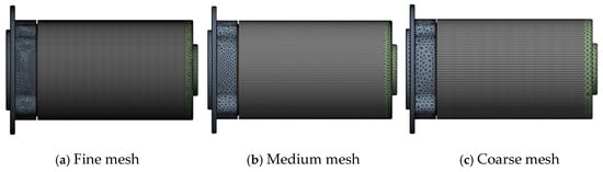
Figure 6.
Grid independence verification.
2.4. Establish Simulation Database
There are 42 FEA models that bolt preload varies from 30 N to 80 N with the groove depth varying from 0.6 mm to 0.9 mm. The results used for evaluation are CP (contact pressure), CA (contact area), and σ (O-ring von stress) [54,55,56]. The stress distribution of the O-ring when H = 0.8 mm with bolt preload 80 N is shown in Figure 7. The maximum von Mises stress is 1.17 MPa in the center of the O-ring section, which is lower than the tensile yield stress 5.929 MPa. The section of the O-ring shows that at the chamfer location, there are some small protrusions on the inner O-ring surface.
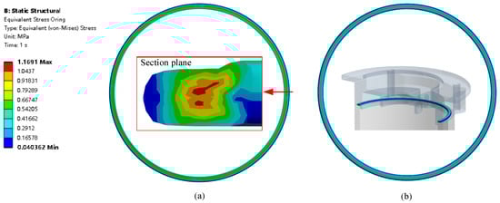
Figure 7.
O-ring stress distribution: (a) O-ring CS1 side surface stress distribution and (b) O-ring CS2 side surface stress distribution.
Contact pressure is very important for sealing performance. O-ring has three contact surfaces, which are shown in Figure 2b and are CS1, CS2, and CS3. The contact pressure distribution of CS1 is shown in Figure 8a, in which the max contact pressure is 1.58 Mpa, while CP2 is 1.28 MPa in Figure 8b. The max contact pressure of CS 3 is 0.89 MPa as shown in Figure 8c.
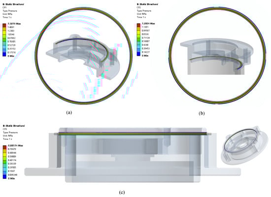
Figure 8.
Contact pressure distribution: (a) CS1 contact pressure; (b) CS2 contact pressure; (c) CS3 contact pressure.
Through the above calculation, the results of the physical quantities related to the O-ring seal are obtained when the groove depth is different and the preload varies. The data are chaotic as generated by the ANSYS workbench software. In order to cluster the data, a suitable ML algorithm was introduced in this study.
2.5. Machine Learning Algorithms
Looking back on the history of scientific development, it is possible to distinguish four scientific discovery methodologies: (1) experiments, (2) mathematical modeling, (3) computer simulation, and (4) data analytics [57]. Figure 9 illustrates these four paradigms.
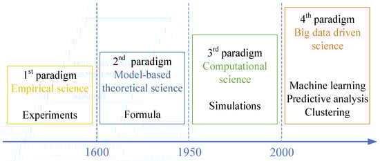
Figure 9.
Four existing paradigms for scientific discovery.
Artificial intelligence (AI) refers to a system with certain intelligence created by humans that can perform tasks that usually require human intelligence. These tasks include but are not limited to learning, reasoning, problem-solving, knowledge representation, planning, navigation, natural language processing, pattern recognition, and learning from experience. Machine learning belongs to AI which involves the use of mathematical and statistical methods to enable machines to learn from given data. These technologies include supervised, semi-supervised, unsupervised, and deep learning [58,59].
2.6. Data Driven by Hierarchical Clustering
Hierarchical clustering (HC) is a collection of closely related cluster algorithms that build hierarchies of clusters. Hierarchical clustering is unsupervised learning from ML which is used when there is no labeled data; it includes two basic approaches, agglomerative and divisive clustering [60]. In this paper, use the first one and it is described in Table 4 according to relevant references [61].
Table 4.
Agglomerative hierarchical clustering algorithm.
The core of unsupervised learning is the automatic discovery of patterns, structures, and relationships from unlabeled data. Data can be processed and analyzed without the need to label the data. At the same time, unsupervised learning can discover the inherent distribution rules and structural characteristics of data, which helps to deeply understand the nature and relationships of data. Although this method performs well in data preprocessing, anomaly detection, and dimension reduction, it also has some obvious shortcomings. For example, the results are poorly interpretable, parameter selection is difficult, calculation complexity is high, etc. Agglomerative clustering follows a bottom-up strategy in which each instance starts its own cluster. The key point is to choose the cluster merging method. There are minimum distance method, maximum distance method, and average distance method in Figure 10.
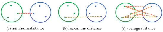
Figure 10.
Schematic diagram of 3 cluster spacing metrics.
The two class clusters are defined as M and N, the data points they contain as P and P’, and the set of points they contain are denoted as CM and CN; then, the formulas described in Figure 10 are Formulas (3)–(5), and the distance between points is calculated according to the Euclidean distance according to Formula (6) [62].
In this paper, Formula (3) calculates the distance, and S is used to represent the sample set. First, each sample is divided into a cluster, and then the distance between any two clusters is calculated, and the cluster with the smallest distance is merged until three clusters appear [63]. The flow chart in Figure 11 describes the details of how HC works on the simulation database.
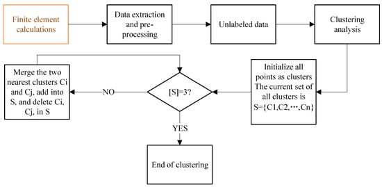
Figure 11.
Agglomerative hierarchical clustering flow chart.
To transform hierarchical clustering into supervised learning, after labeling the minimum data as groove depth from step 1 to step 6, the second cluster was labeled as preload from steps 7 to 11. Through these two methods, unsupervised learning transitioned to supervised learning, and an interpretable cluster was obtained. This method solves the shortcomings of unsupervised learning. At this point, the chaotic data were divided into three categories as in Figure 12: cluster 1 was groove depth (from C1 to C7), cluster 2 was preload (from C8 to C14), and cluster 3 was other data, which were the simulation results.
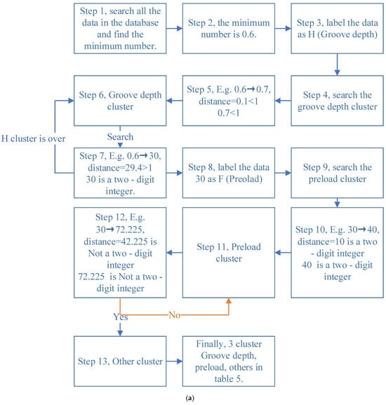
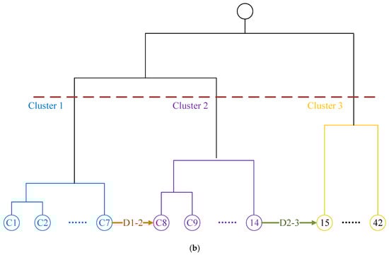
Figure 12.
Clustering process: (a) schematic diagram of labeled clustering principle and (b) the clustering tree of hierarchical clustering.
According to the improved hierarchical clustering algorithm of explainable machine learning, 42 finite element analysis models clustered separately, and the obtained results clustered with labels. All the results are organized in Table 5.
Table 5.
Operating parameters and simulation results.
The data are categorized in Table 5 with the same preload with different groove depths. It is hard to choose among 42 design schemes, which is better as the results show different trends. To overcome this problem, in the next section, a multi-objective double-layer progressive optimization method is developed based on the machine learning algorithm, which is labeled the HC and TOPSIS optimization algorithm. This method considers the simulation result data of O-ring stress, the maximum contact stress, and contact area under different operating parameters.
2.7. Double-Layer Progressive Optimization Method
The double-layer progressive optimization method is based on the TOPSIS method as the parameters change in different trends. TOPSIS is a widely used method of multi-objective decision making to optimize parameters. The weight of each evaluation index was calculated by the entropy method.
As Figure 13 shows, the 3D model with different groove depths was built by computer 3D design software ANSYS SpaceClaim 2023 R2. Then, the model was imported into ANSYS for FEM analysis, element size was set as Figure 6b shows with the medium mesh in Table 3. The preload was started with a bolt preload of 30 Newton; an FEM model was added every 10 Newton until it stopped at 80 Newton. According to the above settings, 42 finite element analysis models were developed that consumed around 126 h. The O-ring stress (σ), O-ring contact surface pressure (CP), and O-ring contact surface area (CA) were obtained. These data make up the first layer of the dataset as Figure 13 and Figure 14’s blue squares show.
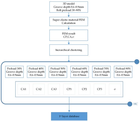
Figure 13.
FEM calculation flow chart.
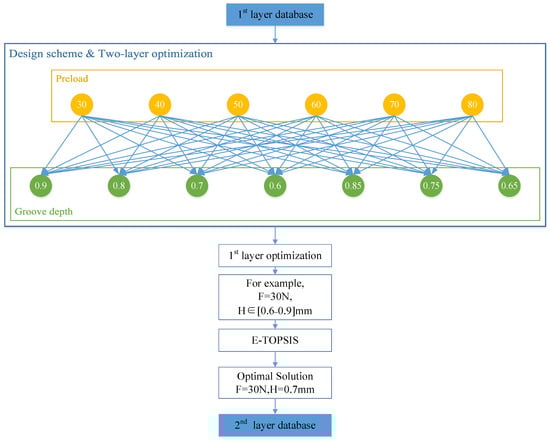
Figure 14.
First layer database optimization flow chart.
After the first layer database was ready, these data were clustered by HC, and then optimized for the first layer through the cross combination of bolt preload and groove depth. This database was transferred to the E-TOPSIS model to optimize the best design scheme for each group. In this section, the simulation result defines PIS (positive ideal solution) and NIS (negative ideal solution). According to the sealing requirements, CP and CA are PIS, and σ is NIS.
After first layer optimization, the optimal design of each preload group with different groove depths was screened out and transferred to the second layer database established in Table 6.
Table 6.
Second layer database.
The basic data of the second layer optimization was formed by the E-TOPSIS method. Finally, the best design scheme was preload 80 N with a groove depth of 0.8 mm as Figure 15 shows.
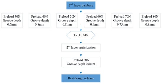
Figure 15.
Second layer database optimization flow chart.
2.7.1. The TOPSIS Method
The TOPSIS method calculates the similarity of each data point based on the distance of the data point to the CA and CP (positive ideal solution) and the O-ring stress (negative ideal solution). The following is the workflow of this method:
Step 1: Establish the original FEA result matrix.
This matrix includes values of evaluation indices under various groove depths.
where Ai (i = 1, 2, 3, …, m) is the ith value of H, and Cj (j = 1, 2, 3, …, n) is the jth evaluation index (i.e., CP, CA, and σ).
Step 2: Normalize the FEA result matrix.
Step 3: Through the entropy method, build the weighted normalized decision matrix.
where wj is the weight for index Cj in Figure 14.
Step 4: Determine the PIS and the NIS by the method below.
where J1 is the cost attributes and J2 is the benefit attributes, respectively. For example, CP is a benefit attribute that should increase.
Step 5: Compute the distances of each data to the NIS and the PIS.
Calculate the distance to the PIS by Formula (12), where is the value of the jth element of PIS.
Calculate the distance to the NIS by Formula (13), is the value of the jth element of NIS.
Step 6: Obtain the similarity of each alternative to the ideal solution.
In Formula (14), Ci* ∈ [0, 1].
Step 7: Select the design scheme with closest to 1 as optimal design.
2.7.2. The Entropy Method
The entropy method calculates the weights of indices according to the amount of information. It provides the weights for TOPSIS including five steps:
Step 1: Normalize the rating matrix, that is, the simulation results. It includes CP, CA, and σ.
For benefit indices (CP3, CP2, CP1, CA3, CA2, and CA1):
For cost indices (σ):
Step 2: Calculate the contribution of the ith alternative in the jth index
Step 3: Compute entropy for each index, Ej ∈ [0, 1]
Step 4: Compute (degree of divergence) according to Ej
Step 5: Compute the weight of CP, CA, and σ
3. Results and Discussion
The simulation time is 126 h following a computational analysis using ANSYS Workbench 2023 R2 on a workstation equipped with an Intel® Xeon® W-2275 processor (3.30 GHz) and 256 GB RAM. The generated simulation data points are clustered by running relevant Python code in PyCharm 2024.2.1 (Community Edition). The data generated by the finite element method are random and disorderly, which makes finding correlations in these data and obtaining optimal designs under the given conditions difficult.
3.1. Calculate the Best Design Solution
After optimizing the first layer of data, the optimization results are transferred to the next layer for secondary optimization so as to find the best design solution among the 42 designs.
Table 6 shows the second layer database for optimization with varying parameters, which are CP, CA, and σ, under various groove depths and preloads in order to find the best design of these six designs. Therefore, the second layer of data is optimized again with TOPSIS.
The similarities and corresponding ranks of the second database are listed in Table 7. The optimal design is DP 37 Pi is the largest among all the designs. The similarities of DP37 and DP34 are very close to each other. Figure 16 shows the relationship between these parameters.
Table 7.
Similarities and rankings of different designs.
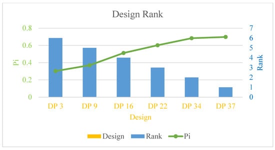
Figure 16.
Similarities and rankings of different designs.
3.2. Experimental Verification
According to Figure 16, the optimal design scheme is DP37. Among all the optimal design schemes, the optimal groove depth of 0.8 mm appeared three times, which is the highest in frequency. By comparing the three design schemes of DP37, DP16, and DP9, under the premise of the same groove depth, the greater the bolt preload, the higher the ranking. Based on the above, a prototype was manufactured according to the parameter of DP37 to test the waterproof sealing performance.
Based on the data of DP37 in Table 6, CP3 = 890.458 kPa; CP2 = 1285.460 kPa; CP1 = 1575.152 kPa. The contact pressures all exceed a water pressure of 15 kPa. The simulation results indicate that the waterproof requirement can be met.
In order to test the sealing structure reliability of the combination optimization method, this study adopts a waterproof sealing test, which has the advantages of low price and cost, and easy implementation. According to IEC 60529 and ISO 20653:2013, IPX8 is more severe than IPX7, defined as a waterproof test under 1.5 m water for 1 h [64].
The waterproof test was carried out by manufacturing a motor prototype with the sealing structure parameters in DP 37 and putting it into a basket under 1.5 m water in a water tank as Figure 17 shows. All the gaps were sealed with sealant except for the O-ring seal construction.
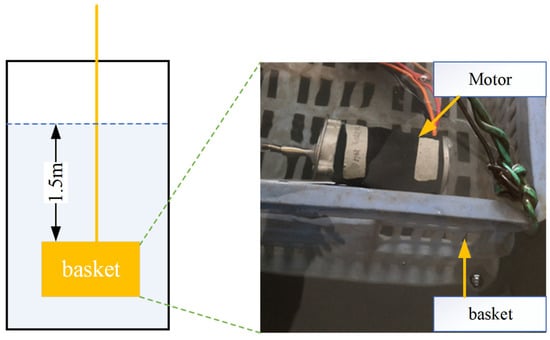
Figure 17.
IPX8 waterproof test.
Gravity, which causes the fluid pressure in a closed container, has the relationship of P (water pressure) with the following formula:
is the density of water taken as , g is the acceleration of gravity taken as g = 10 m/s2, and h is the depth of immersion water taken as h = 1.5 m.
From the theoretical calculation, when the basket is immersed underwater at 1.5 m, the water pressure is 15 kPa. The basket with the test motor was submerged 1.5 m under water and kept for 1 h. Then, the motor was picked up, and the water stains on the surface of the motor were wiped off. The motor was put on the test bench for disassembly.
As Figure 18 shows, the rubber surface is clean without water stains, and the motor base is partially clean without water droplets. The inside of the motor is dry, and there are no water droplets or water stains.
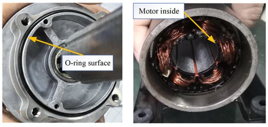
Figure 18.
Check the waterproof performance.
4. Conclusions
In this paper, by marking the minimum value as H, the transformation of the hierarchical clustering of unsupervised learning into an interpretable supervised learning model was carried out. Through this method, the data generated by the finite element method was clustered and turned from disorderly data into clear hierarchical data. Then, the database of each layer was optimized layer by layer, and finally, the best design solution (DP37) among all 42 designs was found. Artificial intelligence algorithms and optimization methods were combined to find optimal results, and the waterproof reliability of the DP37 was verified through the IPX8 waterproof test. The conclusions are summarized as follows:
- This paper improved hierarchical clustering in machine learning and transformed unsupervised learning into supervised learning by labeling the minimum value as the groove depth, storing the distance, and comparing the distance between clusters. The categories of clusters were divided into three categories (groove depth, bolt preload, and other). At the same time, it solved the unexplainably of hierarchical clustering, making the clustered data interpretable. This lays a reliable data foundation for the next step of optimization.
- By introducing the E-TOPSIS method, two layers of data were used for progressive optimization. After two-stage progressive optimization, the best design solution was found to be DP37. The optimization results indicate that the minimum groove depth must be at least 0.7 mm. The groove depth of 0.8 mm appeared three times, which can be given priority consideration during the design process. Under different preloads, the corresponding optimal designed groove depths are different.
- The O-ring contact pressure far exceeded the waterproof level requirements of IPX8. However, the stress on the O-ring part was also high at this time. Based on the data of DP37 in Table 6, CP3 = 890.458 kPa; CP2 = 1285.460 kPa; CP1 = 1575.152 kPa. The contact pressures all exceeded the water pressure of 15 kPa.
- By manufacturing a motor prototype with the sealing structure, the most stringent IPX8 waterproof test was carried out to test the water resistance performance and durability of the sealing structure. The experimental results verified that the waterproof structure is reliable.
The method proposed in this paper enables the rapid and precise selection of optimal design schemes while ensuring clarity and interpretability throughout the entire process. By integrating the finite element method (FEM), the computational efficiency was significantly enhanced, reducing the time, workforce, and material resources traditionally required for experimental validation. Furthermore, in this study, by introducing explainable artificial intelligence (XAI) technology, the limitation of hierarchical clustering methods that produce difficult-to-explain results was addressed. This integration not only improves transparency but also strengthens the reliability of decision making in sealing structural optimization. The method proposed in this paper can easily be applied in motor sealing structure design and extended to other fields such as sealing in aerospace and marine applications.
Author Contributions
Conceptualization, W.Z.; methodology, W.Z.; software, W.Z.; formal analysis, W.Z.; data curation, W.Z.; writing—original draft, W.Z.; writing—review and editing, W.Z.; visualization, Z.X.; supervision, Z.X.; project administration, Z.X.; funding acquisition, Z.X. All authors have read and agreed to the published version of the manuscript.
Funding
The work is supported by the Shenzhen Science and Technology Program (grant number ZDSYS20210623091808026) in China.
Institutional Review Board Statement
Not applicable.
Informed Consent Statement
Not applicable.
Data Availability Statement
The original contributions presented in this study are included in the article. Further inquiries can be directed to the corresponding author.
Conflicts of Interest
The authors declare that there were no conflicts of interest.
Nomenclature
| Symbol | Unit | Implication |
| CP | [kPa] | contact pressure |
| CP1 | [kPa] | contact pressure of Contact surface 1 |
| CP2 | [kPa] | contact pressure of Contact surface 2 |
| CP3 | [kPa] | contact pressure of Contact surface 3 |
| CA | [mm2] | contact area |
| CA1 | [mm2] | contact area of Contact surface 1 |
| CA2 | [mm2] | contact area of Contact surface 2 |
| CA3 | [mm2] | contact area of Contact surface 3 |
| σ | [MPa] | von Mises stress |
| σ1 | [MPa] | principal stresses at x direction |
| σ2 | [MPa] | principal stresses at y direction |
| σ3 | [MPa] | principal stresses at z direction |
| E | [MPa] | Young’s modulus |
| μ | [-] | Poisson’s Ratio |
| Rp0.2 | [MPa] | Tensile Yield Strength |
| Rm | [MPa] | Tensile Ultimate Strength |
| CS1 | [-] | Contact surface 1 |
| CS2 | [-] | Contact surface 2 |
| CS3 | [-] | Contact surface 3 |
| CS4 | [-] | Contact surface 4 |
| CS5 | [-] | Contact surface 5 |
| μk | [-] | kinetic frictional coefficient |
| P | [kPa] | water pressure |
| g | [m/s2] | Earth’s gravity |
| h | [m] | submersion in water depths |
| H | [mm] | groove depth |
| x, y, z | [m] | Cartesian coordinates |
| COF | [-] | coefficient of friction |
| HC | [-] | hierarchical clustering |
| ML | [-] | machine learning |
| XAI | [-] | explainable artificial intelligence |
| NBR | [-] | nitrile butadiene rubber |
| ρ | [kg/m3] | water density |
| FEM | [-] | finite element method |
| IP | [-] | Ingress Protection |
| NIS | [-] | negative ideal solution |
| PIS | [-] | positive ideal solution |
| TOPSIS | [-] | Technique for Order Preference by Similarity to an Ideal Solution similarity to ideal solution |
References
- Chan, C.K.; Chang, C.C.; Yang, I.C.; Shueh, C.; Kuan, C.K.; Sheng, A.; Wu, L.H. A differential pumping system to temporarily seal a leaking, rotatable ConFlat flange. Vacuum 2018, 147, 72–77. [Google Scholar] [CrossRef]
- Aghdasi, A.H.; Khonsari, M.M. Friction behavior of Radial Shaft Sealing Ring subjected to unsteady motion. Mech. Mach. Theory 2021, 156, 104171. [Google Scholar] [CrossRef]
- Wei, W.; Liu, H.; Guo, C.; Jiang, H.; Ouyang, X. Effect of vibration on reciprocating sealing performance. Tribol. Int. 2023, 178, 108031. [Google Scholar] [CrossRef]
- De Groh, H.; Daniels, C.; Dever, J.; Miller, S.; Waters, D.; Finkbeiner, J.; Dunlap, P.; Steinetz, B. Space Environment Effects on Silicone Seal Materials. 2010. Available online: https://ntrs.nasa.gov/citations/20100029591 (accessed on 8 April 2025).
- Yan, H.; Xu, X.; Yao, X.; Qu, T.; Yang, Y. Design of fabric rubber composite seals with multilevel structure using machine learning method. Compos. Part A Appl. Sci. Manuf. 2024, 180, 108053. [Google Scholar] [CrossRef]
- Dong, Y.; Yang, H.; Yan, H.; Yao, X. Design and characteristics of fabric rubber sealing based on microchannel model. Compos. Struct. 2019, 229, 111463. [Google Scholar] [CrossRef]
- Xu, X.; Yao, X.; Dong, Y.; Yang, H.; Yan, H. Mechanical behaviors of non-orthogonal fabric rubber seal. Compos. Struct. 2021, 259, 113453. [Google Scholar] [CrossRef]
- Guo, J.; Zhou, Q.; Tan, X.; Chen, J.; Wang, Y.; Lin, Y. Study on sealing performance and optimization design of a new type non-standard seal strip of submarine pipeline maintenance dry cabin. Ocean. Eng. 2024, 292, 116508. [Google Scholar] [CrossRef]
- Cheng, G.; Guo, F.; Zang, X.; Zhang, Z.; Jia, X.; Yan, X. Failure analysis and improvement measures of airplane actuator seals. Eng. Fail. Anal. 2022, 133, 105949. [Google Scholar] [CrossRef]
- Zhang, Y.; Zhang, N.; Cui, B.; Guo, Q. Failure analysis and structural improvement of helicopter landing gear seals based on experiments and three-dimensional numerical simulation. Eng. Fail. Anal. 2024, 163, 108596. [Google Scholar] [CrossRef]
- Wu, J.-B.; Li, L.; Wang, P.-J. Effect of stress relaxation on the sealing performance of O-rings in deep-sea hydraulic systems: A numerical investigation. Eng. Sci. Technol. Int. J. 2024, 51, 101654. [Google Scholar] [CrossRef]
- Yang, M.; Xia, Y.-M.; Ren, Y.; Zhang, B.-W.; Wang, Y. Design of O-ring with skeleton seal of cutter changing robot storage tank gate for large diameter shield machine. Tribol. Int. 2023, 185, 108591. [Google Scholar] [CrossRef]
- Zhang, Z.; Wu, D.; Pang, H.; Liu, Y.; Wei, W.; Li, R. Extrusion-occlusion dynamic failure analysis of O-ring based on floating bush of water hydraulic pump. Eng. Fail. Anal. 2020, 109, 104358. [Google Scholar] [CrossRef]
- Xing, Y.; Zhai, F.; Li, S.; Yu, X.; Huang, W. Analytical method for contact characteristics of rubber shaft seals under dynamic eccentricity considering viscous effect. Tribol. Int. 2024, 197, 109816. [Google Scholar] [CrossRef]
- Chen, Z.; Liu, T.; Li, J. The effect of the O-ring on the end face deformation of mechanical seals based on numerical simulation. Tribol. Int. 2016, 97, 278–287. [Google Scholar] [CrossRef]
- Kim, H.-K.; Park, S.-H.; Lee, H.-G.; Kim, D.-R.; Lee, Y.-H. Approximation of contact stress for a compressed and laterally one side restrained O-ring. Eng. Fail. Anal. 2007, 14, 1680–1692. [Google Scholar] [CrossRef]
- Zhou, Z.; Zhang, K.; Li, J.; Xu, T. Finite element analysis of stress and contact pressure on the rubber sealing O-ring. Lubr. Eng. 2006, 31, 86–89. [Google Scholar]
- Karaszkiewicz, A. Geometry and Contact Pressure of an O-Ring Mounted in a Seal Groove. Ind. Eng. Chem. Res. 1990, 29, 2134–2137. [Google Scholar] [CrossRef]
- Dragoni, E.; Strozzi, A. Theoretical analysis of an unpressurized elastomeric O-ring seal inserted into a rectangular groove. Wear 1989, 130, 41–51. [Google Scholar] [CrossRef]
- Fried, I.; Johnson, A.R. Nonlinear computation of axisymmetric solid rubber deformation. Comput. Methods Appl. Mech. Eng. 1988, 67, 241–253. [Google Scholar] [CrossRef]
- George, A.F.; Strozzi, A.; Rich, J.I. Stress fields in a compressed unconstrained elastomeric O-ring seal and a comparison of computer predictions and experimental results. Tribol. Int. 1987, 20, 237–247. [Google Scholar] [CrossRef]
- Shukla, A.; Nigam, H. A numerical-experimental analysis of the contact stress problem. J. Strain Anal. Eng. Des. 1985, 20, 241–245. [Google Scholar] [CrossRef]
- Zhou, C.; Zheng, Y.; Hua, Z.; Mou, W.; Liu, X. Recent insights into hydrogen-induced blister fracture of rubber sealing materials: An in-depth examination. Polym. Degrad. Stab. 2024, 224, 110747. [Google Scholar] [CrossRef]
- Zhou, C.; Liu, X.; Zheng, Y.; Hua, Z. A comprehensive review of hydrogen-induced swelling in rubber composites. Compos. Part B Eng. 2024, 275, 111342. [Google Scholar] [CrossRef]
- Clute, C.; Balasooriya, W.; Cano Murillo, N.; Theiler, G.; Kaiser, A.; Fasching, M.; Schwarz, T.; Hausberger, A.; Pinter, G.; Schlögl, S. Morphological investigations on silica and carbon-black filled acrylonitrile butadiene rubber for sealings used in high-pressure H2 applications. Int. J. Hydrog. Energy 2024, 67, 540–552. [Google Scholar] [CrossRef]
- Yamabe, J.; Koga, A.; Nishimura, S. Failure behavior of rubber O-ring under cyclic exposure to high-pressure hydrogen gas. Eng. Fail. Anal. 2013, 35, 193–205. [Google Scholar] [CrossRef]
- Porter, C.; Zaman, B.; Pazur, R. A critical examination of the shelf life of nitrile rubber O-Rings used in aerospace sealing applications. Polym. Degrad. Stab. 2022, 206, 110199. [Google Scholar] [CrossRef]
- Morrell, P.R.; Patel, M.; Skinner, A.R. Accelerated thermal ageing studies on nitrile rubber O-rings. Polym. Test. 2003, 22, 651–656. [Google Scholar] [CrossRef]
- Hussain, A.; Ullah, K.; Senapati, T.; Moslem, S. Energy supplier selection by TOPSIS method based on multi-attribute decision-making by using novel idea of complex fuzzy rough information. Energy Strategy Rev. 2024, 54, 101442. [Google Scholar] [CrossRef]
- Hu, M.; Sun, D.; Sun, G.; Sun, Y.; Ouyang, J. Performance study on anti-weather aging combinations for high-content polymer modified asphalt and comparison by improved multi-scale mathematical TOPSIS method. Constr. Build. Mater. 2023, 407, 133357. [Google Scholar] [CrossRef]
- Chen, C.; Ran, D.; Yang, Y.; Hou, H.; Peng, C. TOPSIS based multi-fidelity Co-Kriging for multiple response prediction of structures with uncertainties through real-time hybrid simulation. Eng. Struct. 2023, 280, 115734. [Google Scholar] [CrossRef]
- Sun, H.; Yang, Z.; Li, J.; Ding, H.; Lv, P. Performance evaluation and optimal design for passive turbulence control-based hydrokinetic energy harvester using EWM-based TOPSIS. Energy 2024, 298, 131377. [Google Scholar] [CrossRef]
- Dwivedi, P.P.; Sharma, D.K. Evaluation and ranking of battery electric vehicles by Shannon’s entropy and TOPSIS methods. Math. Comput. Simul. 2023, 212, 457–474. [Google Scholar] [CrossRef]
- Wang, Z.; Zhong, Y.; Chai, S.-L.; Niu, S.-F.; Yang, M.-L.; Wu, G.-R. Product design evaluation based on improved CRITIC and Comprehensive Cloud-TOPSIS—Applied to automotive styling design evaluation. Adv. Eng. Inform. 2024, 60, 102361. [Google Scholar] [CrossRef]
- Li, J.; Ren, Y.; Ma, X.; Wang, Q.; Ma, Y.; Yu, Z.; Li, J.; Ma, M.; Li, J. Comprehensive evaluation of the working mode of multi-energy complementary heating systems in rural areas based on the entropy-TOPSIS model. Energy Build. 2024, 310, 114077. [Google Scholar] [CrossRef]
- Swathi, B.; Vidjeapriya, R. A multi-criterial optimization of low-carbon binders for a sustainable high-strength concrete using TOPSIS. Constr. Build. Mater. 2024, 425, 135992. [Google Scholar] [CrossRef]
- Wang, D.; Sun, H.; Ge, Y.; Cheng, J.; Li, G.; Cao, Y.; Liu, W.; Meng, J. Operation effect evaluation of grid side energy storage power station based on combined weight TOPSIS model. Energy Rep. 2024, 11, 1993–2002. [Google Scholar] [CrossRef]
- Sabry, I.; Hewidy, A.M.; Naseri, M.; Mourad, A.-H.I. Optimization of process parameters of metal inert gas welding process on aluminum alloy 6063 pipes using Taguchi-TOPSIS approach. J. Alloys Metall. Syst. 2024, 7, 100085. [Google Scholar] [CrossRef]
- Kovari, A. Explainable AI chatbots towards XAI ChatGPT: A review. Heliyon 2025, 11, e42077. [Google Scholar] [CrossRef]
- Nikiforidis, K.; Kyrtsoglou, A.; Vafeiadis, T.; Kotsiopoulos, T.; Nizamis, A.; Ioannidis, D.; Votis, K.; Tzovaras, D.; Sarigiannidis, P. Enhancing transparency and trust in AI-powered manufacturing: A survey of explainable AI (XAI) applications in smart manufacturing in the era of industry 4.0/5.0. ICT Express 2025, 11, 135–148. [Google Scholar] [CrossRef]
- Hu, J.; Zhu, K.; Cheng, S.; Kovalchuk, N.M.; Soulsby, A.; Simmons, M.J.H.; Matar, O.K.; Arcucci, R. Explainable AI models for predicting drop coalescence in microfluidics device. Chem. Eng. J. 2024, 481, 148465. [Google Scholar] [CrossRef]
- Versaci, M.; Laganà, F.; Manin, L.; Angiulli, G. Soft computing and eddy currents to estimate and classify delaminations in biomedical device CFRP plates. J. Electr. Eng. 2025, 76, 72–79. [Google Scholar] [CrossRef]
- Laganà, F.; Bibbò, L.; Calcagno, S.; De Carlo, D.; Pullano, S.A.; Pratticò, D.; Angiulli, G. Smart Electronic Device-Based Monitoring of SAR and Temperature Variations in Indoor Human Tissue Interaction. Appl. Sci. 2025, 15, 2439. [Google Scholar] [CrossRef]
- Ma, R.; Sha, J.; Zhang, S.; Zhu, D.; Kang, W.; Liu, J. Fast grouping fusion method of dual carbon monitoring data based on DBSCAN clustering algorithm. Results Eng. 2025, 26, 105057. [Google Scholar] [CrossRef]
- Abdulnassar, A.A.; Nair, L.R. Performance analysis of Kmeans with modified initial centroid selection algorithms and developed Kmeans9+ model. Meas. Sens. 2023, 25, 100666. [Google Scholar] [CrossRef]
- Li, D.X.; Zhao, H.L.; Zhang, S.M.; Wu, C.R.; Liu, X.L.; Zheng, S.J. Finite Element Analysis on the Influence of Back-Up Ring on the Sealing Effect of Rubber O-Ring. Adv. Mater. Res. 2011, 199–200, 1595–1599. [Google Scholar] [CrossRef]
- Chen, S.H.; Jiang, G.Z.; Li, G.F.; Xie, L.X.; Qian, W.Q. Nonlinear Analysis of Rotary Sealing Performance of Rubber O-Ring. Appl. Mech. Mater. 2014, 470, 371–375. [Google Scholar] [CrossRef]
- Zhang, J.; Xie, J. Investigation of Static and Dynamic Seal Performances of a Rubber O-Ring. J. Tribol. 2018, 140, 042202. [Google Scholar] [CrossRef]
- Mooney, M. A Theory of Large Elastic Deformation. J. Appl. Phys. 1940, 11, 582–592. [Google Scholar] [CrossRef]
- Rivlin, R.S. Large Elastic Deformation. of Isotropic Materials IV. Further Development of General Theory. Phil. Trans. R. Soc. A 1948, 241, 379–397. [Google Scholar]
- Sawadogo, M.; Godin, A.; Duquesne, M.; Lacroix, E.; Veillère, A.; Hamami, A.E.A.; Belarbi, R. Investigation of eco-friendly and economic shape-stabilized composites for building walls and thermal comfort. Build. Environ. 2023, 231, 110026. [Google Scholar] [CrossRef]
- Shoji, D.; Ogwezi, B.; Li, V.C. Bendable concrete in construction: Material selection case studies. Constr. Build. Mater. 2022, 349, 128710. [Google Scholar] [CrossRef]
- Alric, J.; Desrochers, A.; Béland, J.-F. Design, optimization and testing of extruded aluminium profiles assembled by mechanical snap-fit. Structures 2022, 41, 836–848. [Google Scholar] [CrossRef]
- Shen, M.; Peng, X.; Xie, L.; Meng, X.; Li, X. Deformation Characteristics and Sealing Performance of Metallic O-rings for a Reactor Pressure Vessel. Nucl. Eng. Technol. 2016, 48, 533–544. [Google Scholar] [CrossRef]
- Yokoyama, K.; Okazaki, M.; Komito, T. Effect of contact pressure and thermal degradation on the sealability of O-ring. JSAE Rev. 1998, 19, 123–128. [Google Scholar] [CrossRef]
- Geni, M. ANSYS Workbench 18.0 Finite Element Analysis: Fundamentals and Applications; China Machine Press: Beijing, China, 2018. [Google Scholar]
- Choudhary, A.; Geoffrey, F.; Tony, H. Artificial Intelligence for Science; World Scientific: Singapore, 2023. [Google Scholar]
- Sarker, I.H. Machine Learning: Algorithms, Real-World Applications and Research Directions. SN Comput. Sci. 2021, 2, 160. [Google Scholar] [CrossRef] [PubMed]
- Xue, J.; Alinejad-Rokny, H.; Liang, K. Navigating micro- and nano-motors/swimmers with machine learning: Challenges and future directions. ChemPhysMater 2024, 3, 273–283. [Google Scholar] [CrossRef]
- Ran, X.; Xi, Y.; Lu, Y.; Wang, X.; Lu, Z. Comprehensive survey on hierarchical clustering algorithms and the recent developments. Artif. Intell. Rev. 2023, 56, 8219–8264. [Google Scholar] [CrossRef]
- Wlodarczak, P. Machine Learning and its Applications, 1st ed.; CRC Press: Boca Raton, FL, USA, 2019; p. 188. [Google Scholar]
- Liu, L.; Zheng, F. An improved cohesive hierarchical clustering for indoor air quality monitoring in smart gymnasium with healthy sport areas. Alex. Eng. J. 2024, 105, 204–217. [Google Scholar] [CrossRef]
- Jia, J.; Ju, S. Clustering-based method for locating critical slip surface using the strength reduction method. Comput. Geotech. 2023, 155, 105241. [Google Scholar] [CrossRef]
- He, Z.; Kwon, D.; Pecht, M. Evaluation of IEC 60529 as a standard for liquid protection assessment of portable electronics. E-Prime Adv. Electr. Eng. Electron. Energy 2025, 12, 100952. [Google Scholar] [CrossRef]
Disclaimer/Publisher’s Note: The statements, opinions and data contained in all publications are solely those of the individual author(s) and contributor(s) and not of MDPI and/or the editor(s). MDPI and/or the editor(s) disclaim responsibility for any injury to people or property resulting from any ideas, methods, instructions or products referred to in the content. |
© 2025 by the authors. Licensee MDPI, Basel, Switzerland. This article is an open access article distributed under the terms and conditions of the Creative Commons Attribution (CC BY) license (https://creativecommons.org/licenses/by/4.0/).