
Development of FSW Process Parameters for Lap Joints Made of Thin 7075 Aluminum Alloy Sheets


Abstract
1. Introduction
1.1. Methods of Controlling the FSW Process
1.2. Parameter Optimization Using a Machine Learning Approach
2. Materials and Methods
3. Development of Process Parameters Using Machine Learning
3.1. Classification
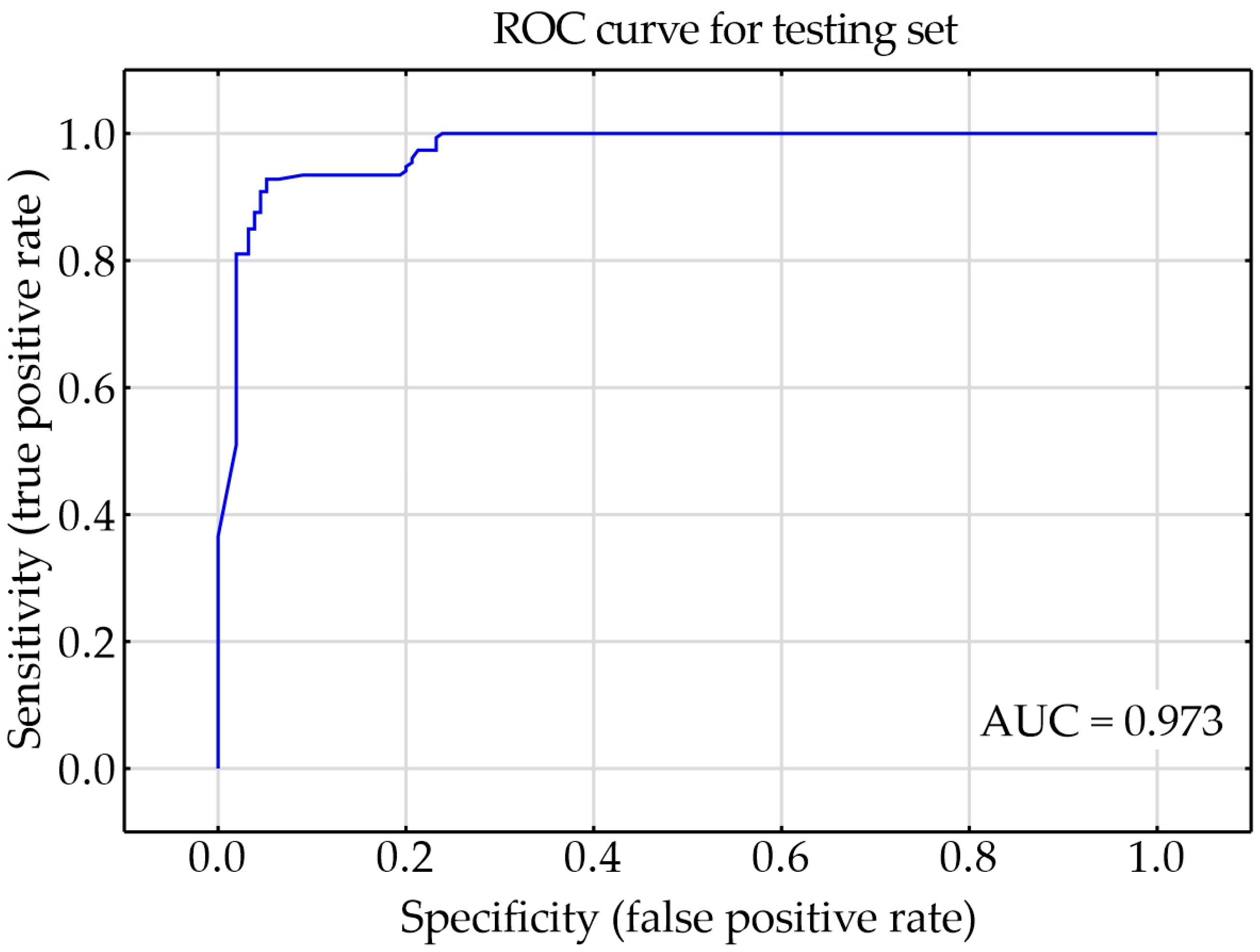
- The largest possible area under the curve (AUC), affecting the quality of the network;
- The largest possible accuracy of the testing set, affecting the quality of the network;
- The smallest possible number of neurons, affecting the level of computation complexity; and
- Types of activation functions as simple as possible, affecting the level of complexity of calculations.
- di—dependent variable,
- yi—predicted output.
- Sensitivity (true positive rate)—the probability of a positive test result, conditioned on the individual truly being positive.
- Specificity (true negative rate)—the probability of a negative test result, conditioned on the individual truly being negative.
- Precision (positive predictive value)—the fraction of relevant instances among the retrieved instances.
- Negative predictive values—the proportion of negative results that are true negative results.
- Accuracy—determines how close a given set of measurements are to their true value.
- TP—true positive, a test result that correctly indicates the presence of a condition or characteristic.
- TN—true negative, a test result that correctly indicates the absence of a condition or characteristic.
- FP—false positive, a test result that wrongly indicates that a particular condition or attribute is present.
- FN—false negative, a test result that wrongly indicates that a particular condition or attribute is absent.
- ω—spindle speed or tool rotation rate in rpm,
- ν—feed rate or tool travel speed in mm/min.
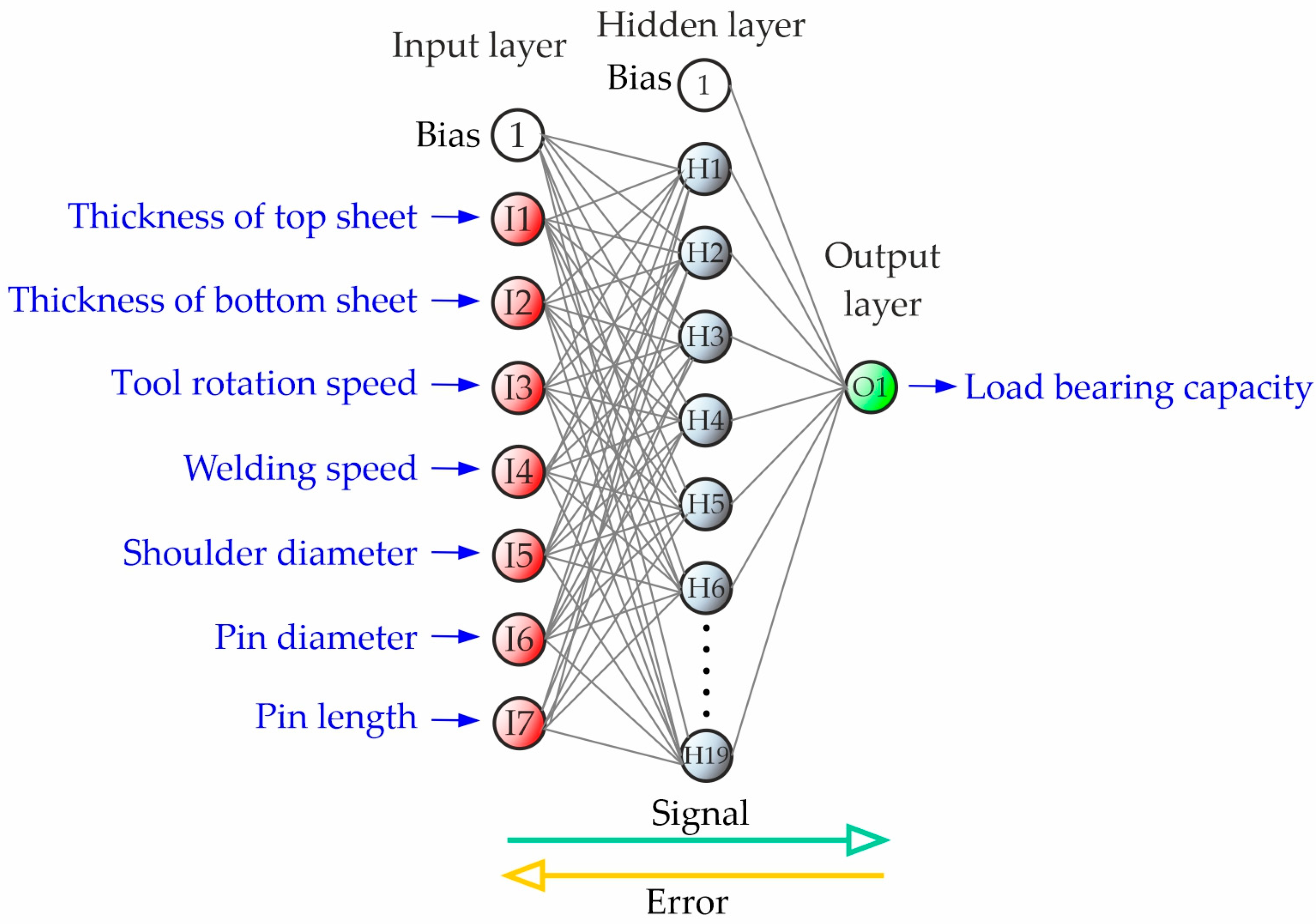
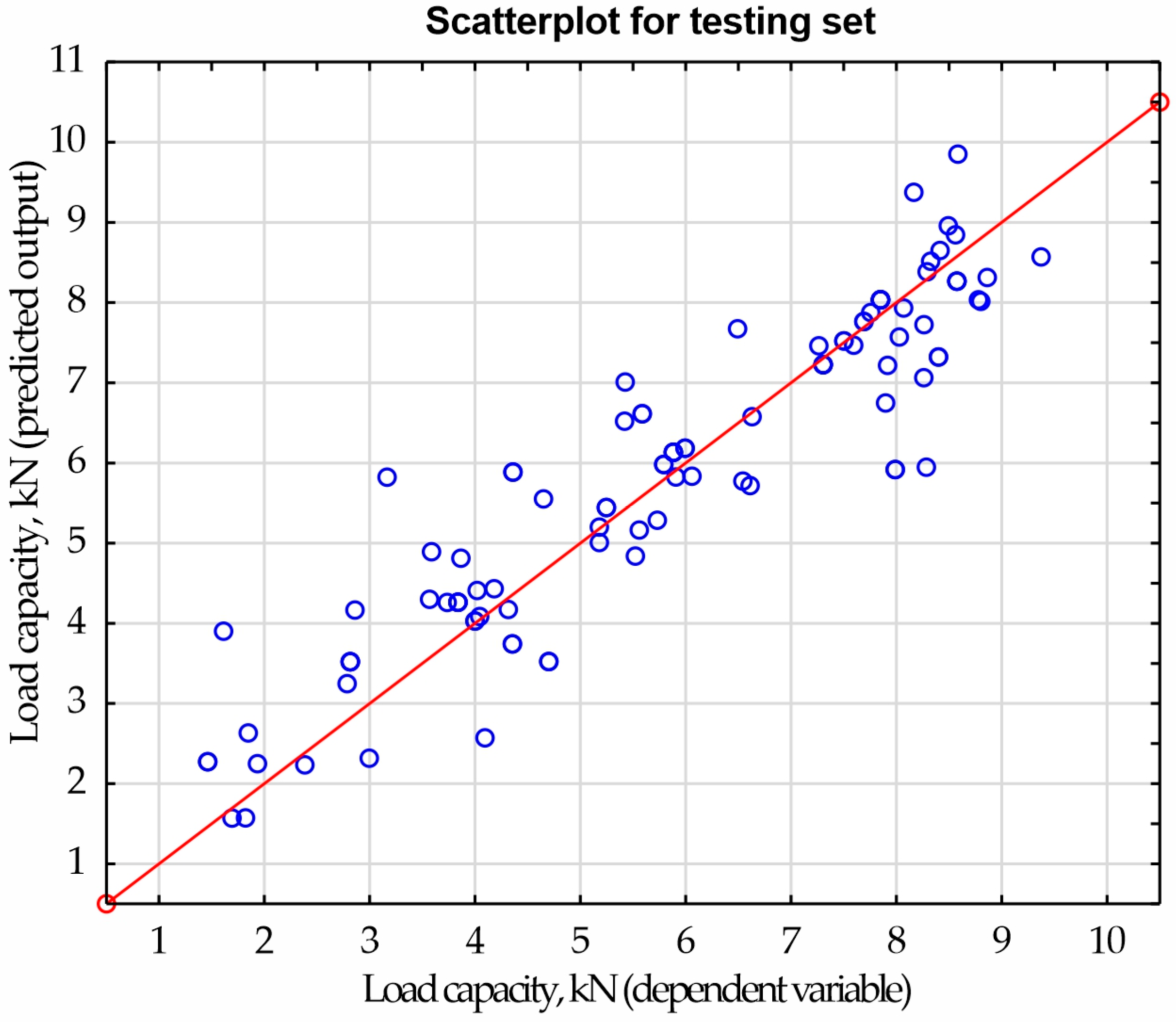
3.2. Regression
- The largest possible accuracy of the testing set, affecting the quality of the network;
- The smallest possible error of the testing set, affecting the network quality;
- The smallest possible number of neurons, affecting the level of computation complexity; and
- Types of activation functions as simple as possible, affecting the level of complexity of calculations.
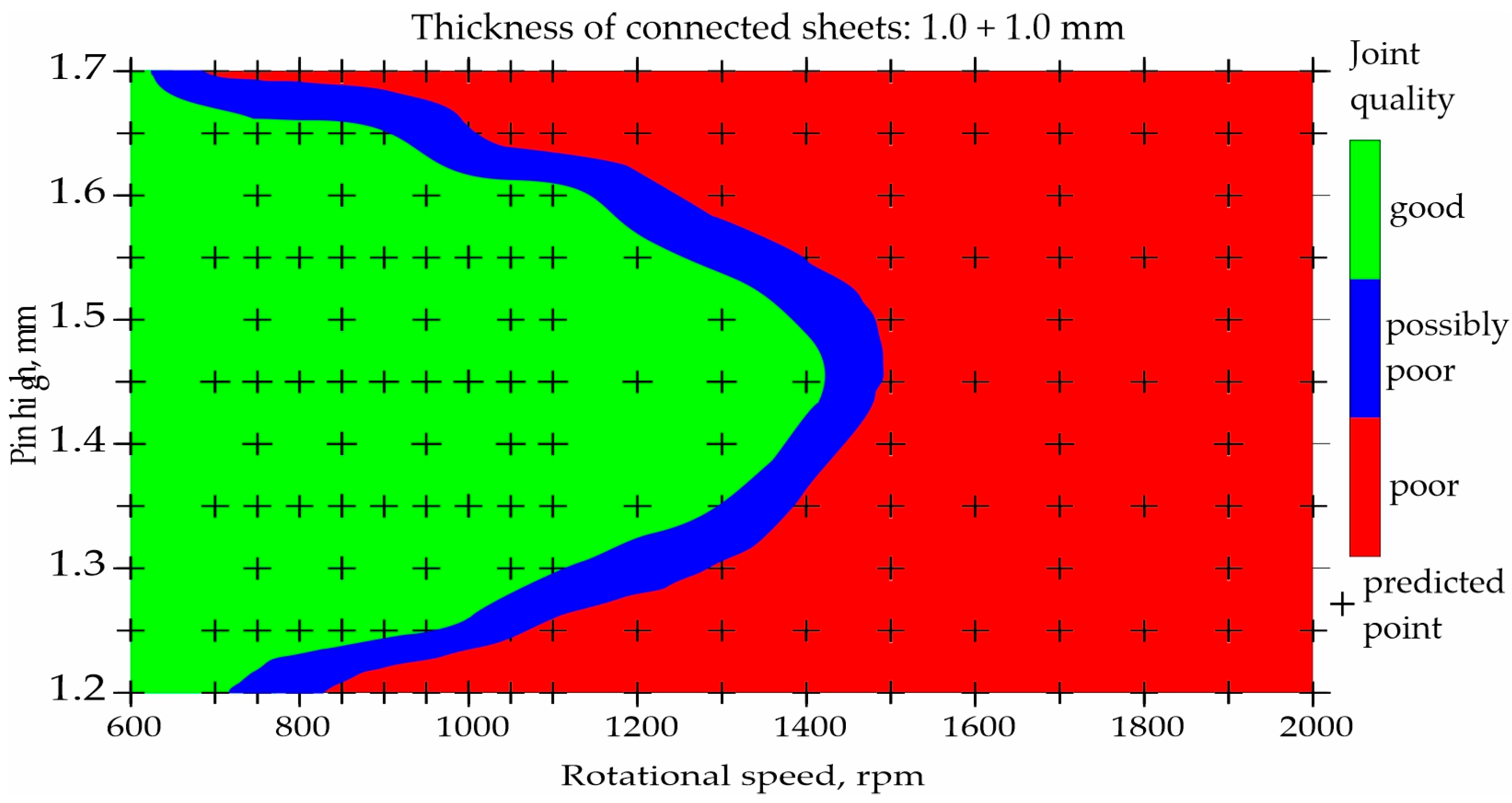
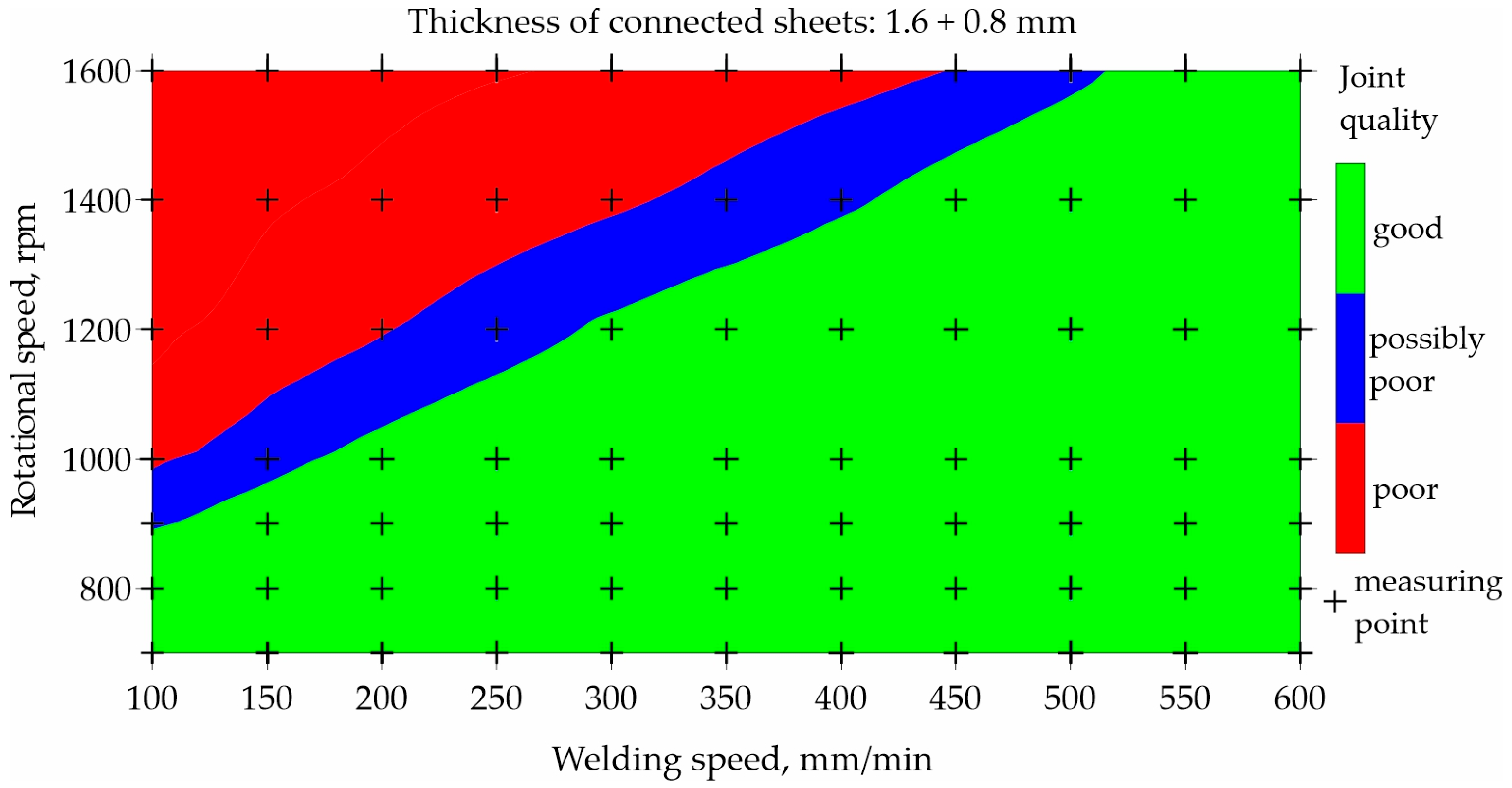
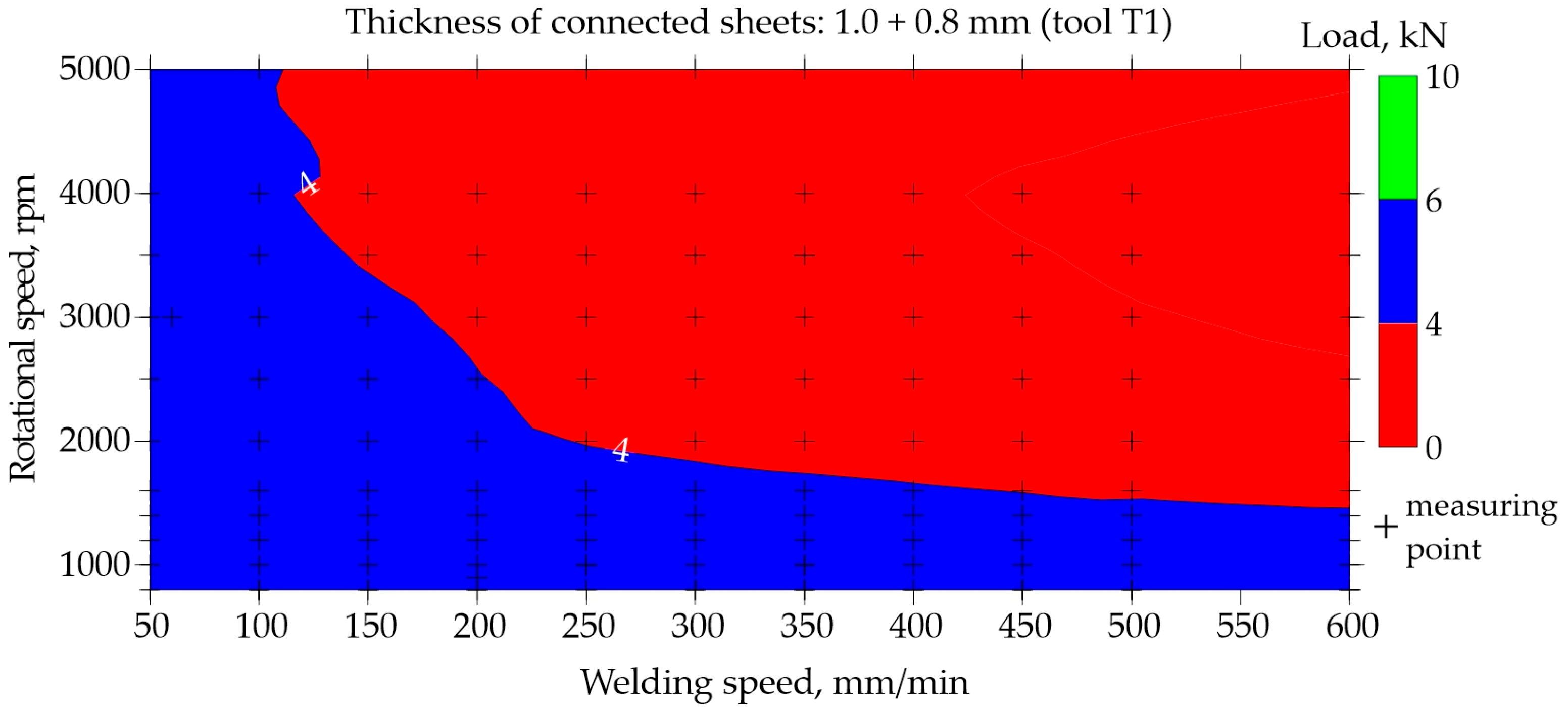
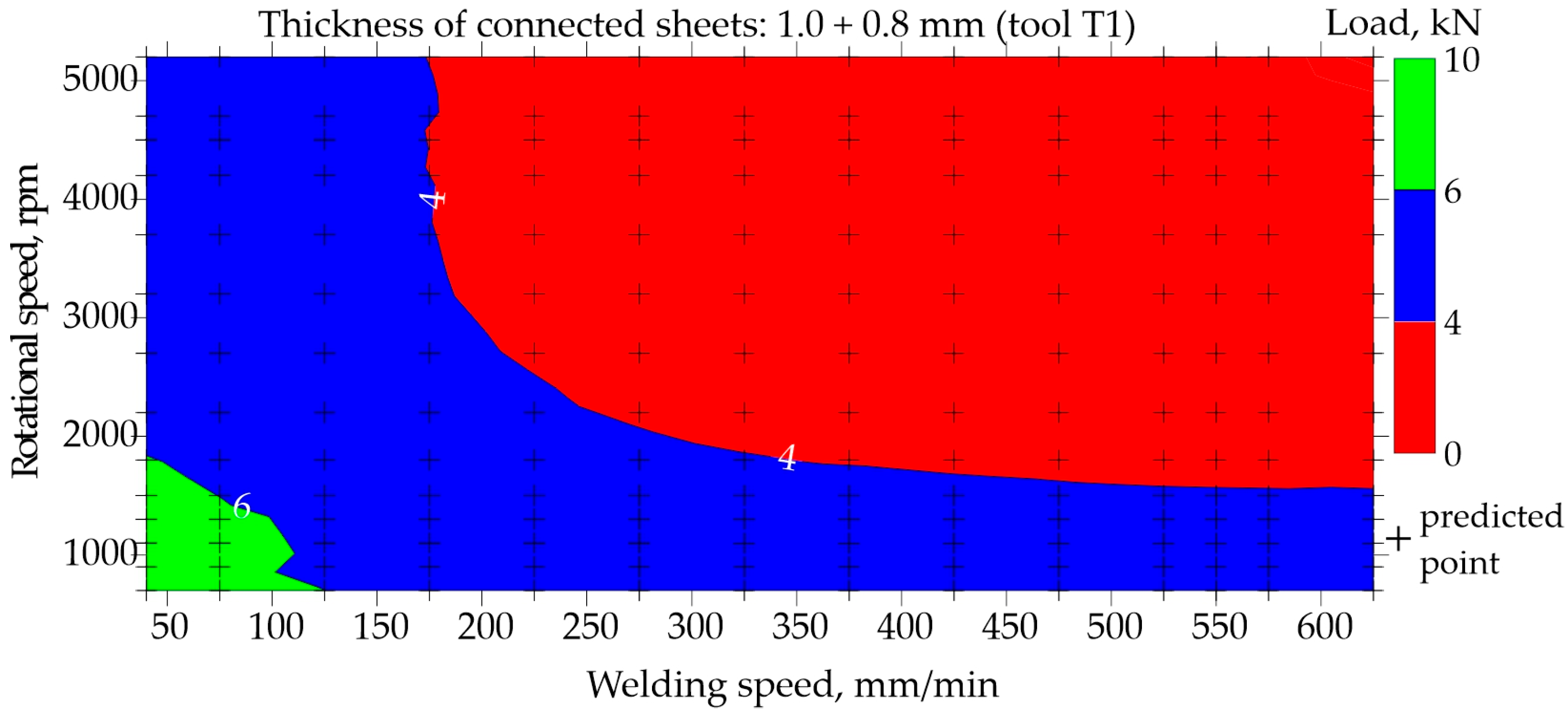
4. Case Study
5. Discussion
- -
- Nonlinearity Modelling: The FSW process is nonlinear and complex, with many variables influencing its results. Artificial neural networks can effectively model complex, non-linear relationships between process parameters and welding results.
- -
- Adaptation to Experimental Data: Due to the ability of ANNs to learn from data, they can be adapted to specific experimental data from the FSW process, enabling precise modelling of process characteristics.
- -
- Process Optimization: ANNs can be used to optimize FSW process parameters. By training the network on experimental data and using it to predict results for various combinations of parameters, optimal welding conditions can be identified.
- -
- Defect Diagnostics and Prediction: ANNs can be used to diagnose the FSW process and predict potential defects. Based on input data (process parameters) and results, the network can indicate areas where quality problems may occur.
- -
- Adaptive Process Control: Using ANNs to monitor the FSW process in real-time and adjust parameters on the fly can improve weld quality and process efficiency.
6. Conclusions
- The selected parameters of FSW process, including rotational speed, welding speed, and joint and tool geometry, which were used as input data for training a neural network, allowed a correctly predicting neural network to be obtained.
- The classification network was trained in just 72 epochs. The AUC of the network was of 0.973. The quality of the validation set was approximately 93.6%. In the confusion matrix for testing set, the errors never exceeded 6%. MLP 7-19-2 topology was used to build the regression network. This result was assessed as satisfactory.
- The regression network was trained in only 184 epochs. The quality of the validation set was approximately 87.1%. MLP 7-19-1 topology was used to build the regression network. This result was also assessed as satisfactory.
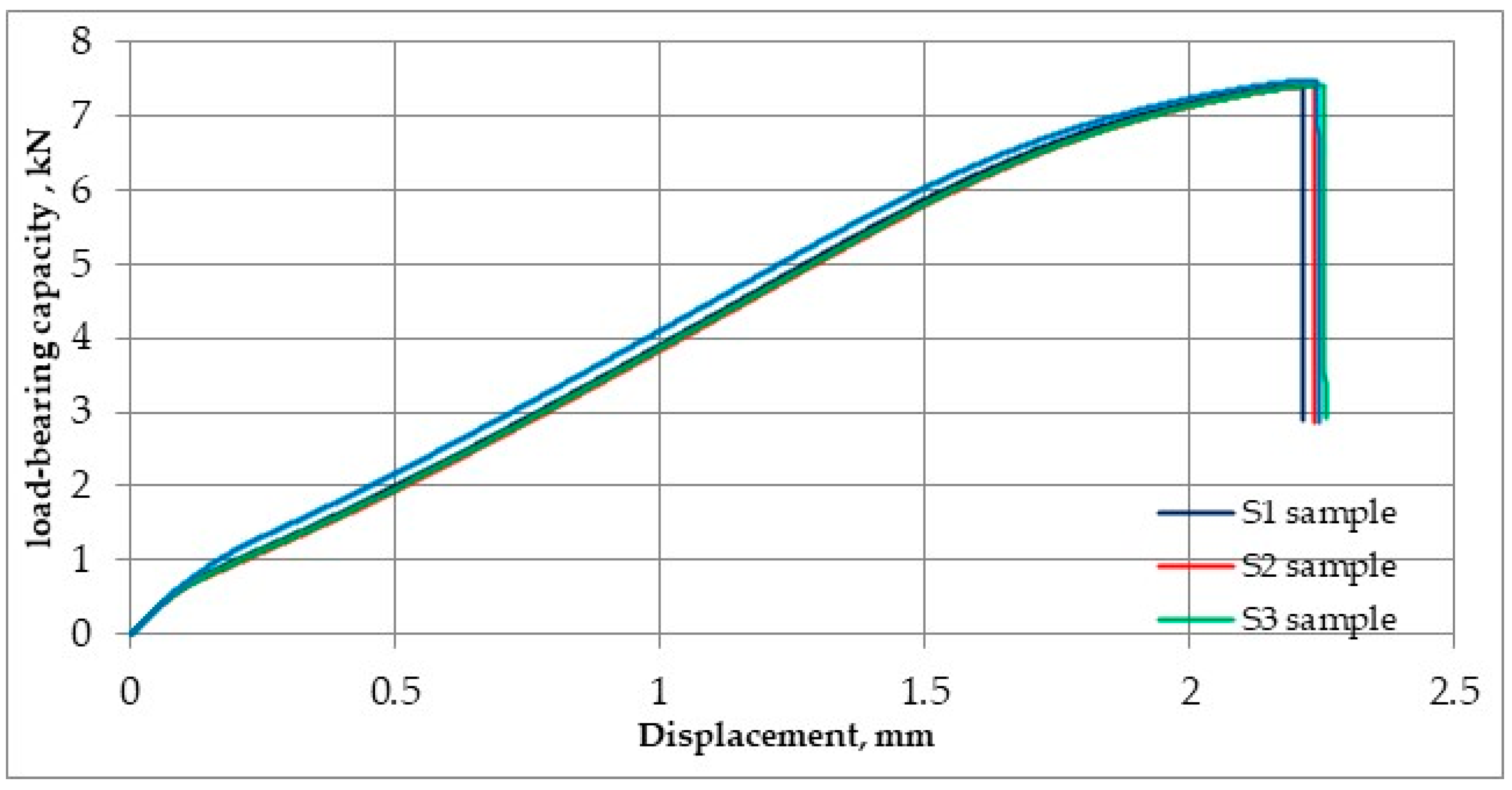
- The case study showed that for the analyzed joint J1, neural networks predicted a 19% lower joint load-bearing capacity than the research showed. This is a safe approach from the design point of view.
Author Contributions
Funding
Institutional Review Board Statement
Informed Consent Statement
Data Availability Statement
Conflicts of Interest
References
- Wright, A.; Munro, T.R.; Hovanski, Y. Evaluating Temperature Control in Friction Stir Welding for Industrial Applications. JMMP 2021, 5, 124. [Google Scholar] [CrossRef]
- Sharma, C.; Dwivedi, D.K.; Kumar, P. Effect of welding parameters on microstructure and mechanical properties of friction stir welded joints of AA7039 aluminum alloy. Mater Des. 2012, 36, 379–390. [Google Scholar] [CrossRef]
- Węglowski, M.S.; Pietras, A.; Węglowska, A. Effect of welding parameters on mechanical and microstructural properties of al 2024 joints produced by friction stir welding. J. KONES Powertrain Transp. 2009, 16, 523–532. [Google Scholar]
- Shashi Kumar, S.; Murugan, N.; Ramachandran, K.K. Identifying the optimal FSW process parameters for maximizing the tensile strength of friction stir welded AISI 316L butt joints. Measurement 2019, 137, 257–271. [Google Scholar] [CrossRef]
- Kadlec, M.; Růžek, R.; Nováková, L. Mechanical behaviour of AA 7475 friction stir welds with the kissing bond defect. Int. J. Fatigue 2015, 74, 7–19. [Google Scholar] [CrossRef]
- Abd Elnabi, M.M.; El Mokadem, A.; Osman, T. Optimization of process parameters for friction stir welding of dissimilar aluminum alloys using different Taguchi arrays. Int. J. Adv. Manuf. Technol. 2022, 121, 3935–3964. [Google Scholar] [CrossRef]
- Chiaranai, S.; Pitakaso, R.; Sethanan, K.; Kosacka-Olejnik, M.; Srichok, T.; Chokanat, P. Ensemble Deep Learning Ultimate Tensile Strength Classification Model for Weld Seam of Asymmetric Friction Stir Welding. Processes 2023, 11, 434. [Google Scholar] [CrossRef]
- Matitopanum, S.; Luesak, P.; Chiaranai, S.; Pitakaso, R.; Srichok, T.; Sirirak, W.; Jirasirilerd, G. A Predictive Model for Weld Properties in AA-7075-FSW: A Heterogeneous AMIS-Ensemble Machine Learning Approach. Intell. Syst. Appl. 2023, 19, 200259. [Google Scholar] [CrossRef]
- Matitopanum, S.; Pitakaso, R.; Sethanan, K.; Srichok, T.; Chokanat, P. Prediction of the Ultimate Tensile Strength (UTS) of Asymmetric Friction Stir Welding Using Ensemble Machine Learning Methods. Processes 2023, 11, 391. [Google Scholar] [CrossRef]
- Ye, X.; Su, Z.; Dahari, M.; Su, Y.; Alsulami, S.H.; Aldhabani, M.S.; Abed, A.M.; Ali, H.E.; Bouzgarrou, S.M. Hybrid modeling of mechanical properties and hardness of aluminum alloy 5083 and C100 Copper with various machine learning algorithms in friction stir welding. Structures 2023, 55, 1250–1261. [Google Scholar] [CrossRef]
- Du, Y.; Mukherjee, T.; Mitra, P.; DebRoy, T. Machine learning based hierarchy of causative variables for tool failure in friction stir welding. Acta Mater. 2020, 192, 67–77. [Google Scholar] [CrossRef]
- Arboretti, R.; Ceccato, R.; Pegoraro, L.; Salmaso, L. Design choice and machine learning model performances. Qual. Reliab. Eng. 2022, 38, 3357–3378. [Google Scholar] [CrossRef]
- Maheshwari, S.; Kar, A.; Alam, Z.; Kumar, L. Deep Neural Network-Based Approach for Modeling, Predicting, and Validating Weld Quality and Mechanical Properties of Friction Stir Welded Dissimilar Materials. JOM 2023, 75, 4562–4578. [Google Scholar] [CrossRef]
- Masoudi Nejad, R.; Sina, N.; Ma, W.; Liu, Z.; Berto, F.; Gholami, A. Optimization of fatigue life of pearlitic Grade 900A steel based on the combination of genetic algorithm and artificial neural network. Int. J. Fatigue 2022, 162, 106975. [Google Scholar] [CrossRef]
- Chai, M.; Liu, P.; He, Y.; Han, Z.; Duan, Q.; Song, Y.; Zhang, Z. Machine learning-based approach for fatigue crack growth prediction using acoustic emission technique. Fatigue Fract. Eng. Mater. Struct. 2023, 46, 2784–2797. [Google Scholar] [CrossRef]
- Ji, S.D.; Jin, Y.Y.; Yue, Y.M.; Gao, S.S.; Huang, Y.X.; Wang, L. Effect of Temperature on Material Transfer Behavior at Different Stages of Friction Stir Welded 7075-T6 Aluminum Alloy. J. Mater. Sci. Technol. 2013, 29, 955–960. [Google Scholar] [CrossRef]
- Khodir, S.A.; Shibayanagi, T. Friction stir welding of dissimilar AA2024 and AA7075 aluminum alloys. Mater. Sci. Eng. B 2008, 148, 82–87. [Google Scholar] [CrossRef]
- Szczucka-Lasota, B.; Węgrzyn, T.; Jurek, A. Aluminum Alloy Welding in Automotive Industry. Transp. Probl. 2020, 15, 67–78. [Google Scholar] [CrossRef]
- Rajakumar, S.; Muralidharan, C.; Balasubramanian, V. Influence of friction stir welding process and tool parameters on strength properties of AA7075-T6 aluminium alloy joints. Mater Des. 2011, 32, 535–549. [Google Scholar] [CrossRef]
- Buffa, G.; Fratini, L.; Shivpuri, R. Finite element studies on friction stir welding processes of tailored blanks. Comput. Struct. 2008, 86, 181–189. [Google Scholar] [CrossRef]
- Lacki, P.; Derlatka, A.; Gałaczyński, T. Selection of basic position in Refill Friction Stir Spot Welding of 2024-T3 and D16UTW aluminum alloy sheets. Arch. Metall. Mater. 2017, 62, 443–449. [Google Scholar] [CrossRef]
- Lacki, P.; Derlatka, A. Strength evaluation of beam made of the aluminum 6061-T6 and titanium grade 5 alloys sheets joined by RFSSW and RSW. Compos. Struct. 2017, 159, 491–497. [Google Scholar] [CrossRef]
- EN 573-3; Aluminium and Aluminium Alloys: Chemical Composition and Form of Wrought Products—Part 3: Chemical Composition and Form of Products. CEN, CEN European Committee for Standardization: Brussels, Belgium, 2007.
- Baum, E.B.; Haussler, D. What Size Net Gives Valid Generalization? Neural Comput. 1989, 1, 151–160. [Google Scholar] [CrossRef]
- Alwosheel, A.; van Cranenburgh, S.; Chorus, C.G. Is your dataset big enough? Sample size requirements when using artificial neural networks for discrete choice analysis. J. Choice Model. 2018, 28, 167–182. [Google Scholar] [CrossRef]
- Arbegast, W.J. Modeling friction stir joining as a metal working process. In Hot Deformation of Aluminum Alloys; Jin, Z., Ed.; TMS: Warrendale, PA, USA, 2003. [Google Scholar]
- Zhou, N.; Song, D.; Qi, W.; Li, X.; Zou, J.; Attallah, M.M. Influence of the kissing bond on the mechanical properties and fracture behaviour of AA5083-H112 friction stir welds. Mater. Sci. Eng. A 2018, 719, 12–20. [Google Scholar] [CrossRef]
- Adamus, K.; Adamus, J.; Lacki, J. Ultrasonic testing of thin walled components made of aluminum based laminates. Compos. Struct. 2018, 202, 95–101. [Google Scholar] [CrossRef]
- Lacki, P.; Adamus, K.; Winowiecka, J. The numerical simulation of aviation structure joined by FSW. Arch. Metall. Mater. 2019, 64, 387–392. [Google Scholar] [CrossRef]


| Joint Type | Top Sheet Metal Thickness tt [mm] | Bottom Sheet Metal Thickness tb [mm] |
|---|---|---|
| J1 | 1.0 | 0.8 |
| J2 | 1.0 | 1.0 |
| J3 | 1.6 | 0.8 |
| Content (wt.%) | |||||||||
|---|---|---|---|---|---|---|---|---|---|
| Cu | Mg | Cr | Zn | Ti | Mn | Si | Fe | Other | Al |
| 1.5 | 2.6 | 0.2 | 5.4 | 0.3 | 0.2 | 0.3 | 0.4 | 0.11 | residue |
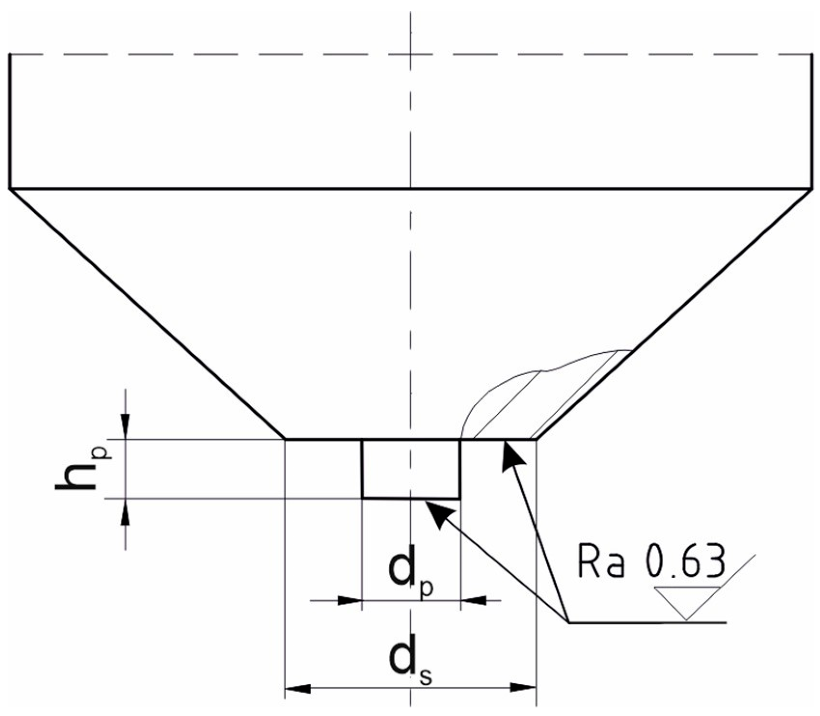
| Tool Type | Shoulder Diameter, ds [mm] | Pin Diameter, dp [mm] | Pin Height, hp [mm] |
|---|---|---|---|
| T1 | 7.0 | 2.0 | 1.20 |
| T2 | 5.0 | 2.0 | 1.20 |
| T3 | 1.6 | 0.8 | 1.10 |
| T4 | 10.0 | 4.0 | 1.20 |
| T5 | 10.0 | 4.0 | 1.26 |
| T6 | 10.0 | 4.0 | 1.56 |
| T7 | 10.0 | 4.0 | 1.30 |
| T8 | 10.0 | 4.0 | 1.40 |
| T9 | 10.0 | 4.0 | 1.50 |
| T10 | 10.0 | 4.0 | 1.60 |
| T11 | 10.0 | 4.0 | 1.84 |
| T12 | 10.0 | 4.0 | 1.86 |
| T13 | 10.0 | 4.0 | 1.88 |
| T14 | 10.0 | 4.0 | 1.90 |
| Type of Joint (Thicknesses of Sheets) | Number of Samples from Experiment | Learning Set | Testing Set | Validation Set |
|---|---|---|---|---|
| 1.0 mm + 0.8 mm | 282 | 198 | 42 | 42 |
| 1.0 mm + 1.0 mm | 228 | 160 | 34 | 34 |
| 1.6 mm + 0.8 mm | 98 | 68 | 15 | 15 |
| Network Type | Number of Neurons in the Hidden Layer | Activation Function in the Hidden Layer | Activation Function in the Output Layer | Learning Algorithm | Error Function | AUC | Accuracy of Learning Set | Accuracy of Testing Set | Accuracy of Validation Set | Number of Epochs |
|---|---|---|---|---|---|---|---|---|---|---|
| RBF | 19 | Gaussian | Linear | RBFT | SSE | 0.506 | 61.7% | 63.5% | 61.3% | - |
| MLP | 19 | Logistic | Linear | GD | SSE | 0.858 | 71.4% | 75.0% | 64.5% | 173 |
| MLP | 19 | Logistic | Linear | CG | SSE | 0.934 | 85.8% | 87.5% | 79.6% | 127 |
| MLP | 19 | Logistic | Softmax | BFGS | Cross Entropy | 0.673 | 51.1% | 50.0% | 38.7% | - |
| MLP | 19 | Exponential | Softmax | BFGS | Cross Entropy | 0.722 | 51.1% | 50.0% | 38.7% | - |
| MLP | 16 | Logistic | Linear | BFGS | SSE | 0.966 | 90.1% | 91.3% | 91.4% | 62 |
| MLP | 19 | Logistic | Linear | BFGS | SSE | 0.973 | 93.2% | 93.5% | 93.6% | 72 |
| MLP | 21 | Logistic | Linear | BFGS | SSE | 0.972 | 92.1% | 92.3% | 88.2% | 84 |
| MLP | 19 | Logistic | Hyperbolic tangent | BFGS | SSE | 0.974 | 91.8% | 90.4% | 87.1% | 55 |
| MLP | 19 | Exponential | Hyperbolic tangent | BFGS | SSE | 0.972 | 89.9% | 93.3% | 90.3% | 64 |
| Prediction | Actual | |||
| Positive | Negative | |||
| Positive | 141 | 8 | Precision: 94.6% | |
| Negative | 12 | 147 | Negative predictive value: 92.5% | |
| Sensitivity: 92.2% | Specificity: 94.8% | Accuracy: 93.5% | ||
| Network Type | Number of Neurons in the Hidden Layer | Activation Function in the Hidden Layer | Activation Function in the Output Layer | Learning Algorithm | Error Function | Accuracy of Learning Set | Accuracy of Testing Set | Error of Testing Set | Accuracy of Validation Set | Number of Epochs |
|---|---|---|---|---|---|---|---|---|---|---|
| RBF | 19 | Gaussian | Linear | RBFT | SSE | 29.4% | 31.4% | 5.1 × 10⁹ | 39.2% | - |
| MLP | 19 | Hyperbolic tangent | Linear | GD | SSE | 85.6% | 87.9% | 0.55 | 82.2% | 284 |
| MLP | 19 | Hyperbolic tangent | Linear | CG | SSE | 36.6% | 39.2% | 2.71 | 31.0% | 4 |
| MLP | 16 | Hyperbolic tangent | Linear | BFGS | SSE | 92.9% | 90.3% | 0.44 | 88.3% | 179 |
| MLP | 19 | Hyperbolic tangent | Linear | BFGS | SSE | 94.8% | 92.5% | 0.35 | 87.1% | 184 |
| MLP | 21 | Hyperbolic tangent | Linear | BFGS | SSE | 93.5% | 90.1% | 0.45 | 84.9% | 160 |
| MLP | 19 | Logistic | Hyperbolic tangent | BFGS | SSE | 93.8% | 89.5% | 0.49 | 80.0% | 244 |
| MLP | 19 | Logistic | Linear | BFGS | SSE | 92.0% | 90.9% | 0.41 | 87.1% | 159 |
Disclaimer/Publisher’s Note: The statements, opinions and data contained in all publications are solely those of the individual author(s) and contributor(s) and not of MDPI and/or the editor(s). MDPI and/or the editor(s) disclaim responsibility for any injury to people or property resulting from any ideas, methods, instructions or products referred to in the content. |
© 2024 by the authors. Licensee MDPI, Basel, Switzerland. This article is an open access article distributed under the terms and conditions of the Creative Commons Attribution (CC BY) license (https://creativecommons.org/licenses/by/4.0/).
Share and Cite
Lacki, P.; Derlatka, A.; Więckowski, W.; Adamus, J. Development of FSW Process Parameters for Lap Joints Made of Thin 7075 Aluminum Alloy Sheets. Materials 2024, 17, 672. https://doi.org/10.3390/ma17030672
Lacki P, Derlatka A, Więckowski W, Adamus J. Development of FSW Process Parameters for Lap Joints Made of Thin 7075 Aluminum Alloy Sheets. Materials. 2024; 17(3):672. https://doi.org/10.3390/ma17030672
Chicago/Turabian StyleLacki, Piotr, Anna Derlatka, Wojciech Więckowski, and Janina Adamus. 2024. "Development of FSW Process Parameters for Lap Joints Made of Thin 7075 Aluminum Alloy Sheets" Materials 17, no. 3: 672. https://doi.org/10.3390/ma17030672
APA StyleLacki, P., Derlatka, A., Więckowski, W., & Adamus, J. (2024). Development of FSW Process Parameters for Lap Joints Made of Thin 7075 Aluminum Alloy Sheets. Materials, 17(3), 672. https://doi.org/10.3390/ma17030672