
Analysis of TRIP Steel HCT690 Deformation Behaviour for Prediction of the Deformation Process and Spring-Back of the Material via Numerical Simulation

Abstract
1. Introduction
2. Materials and Methods
2.1. TRIP Steel HCT690 (EN 10346)
2.2. Methodology of Calculation the Sheet-Metal-Forming Numerical Simulation in PAM-STAMP 2G Software
2.3. Selected Material Computational Models of Numerical Simulation in PAM-STAMP 2G Software
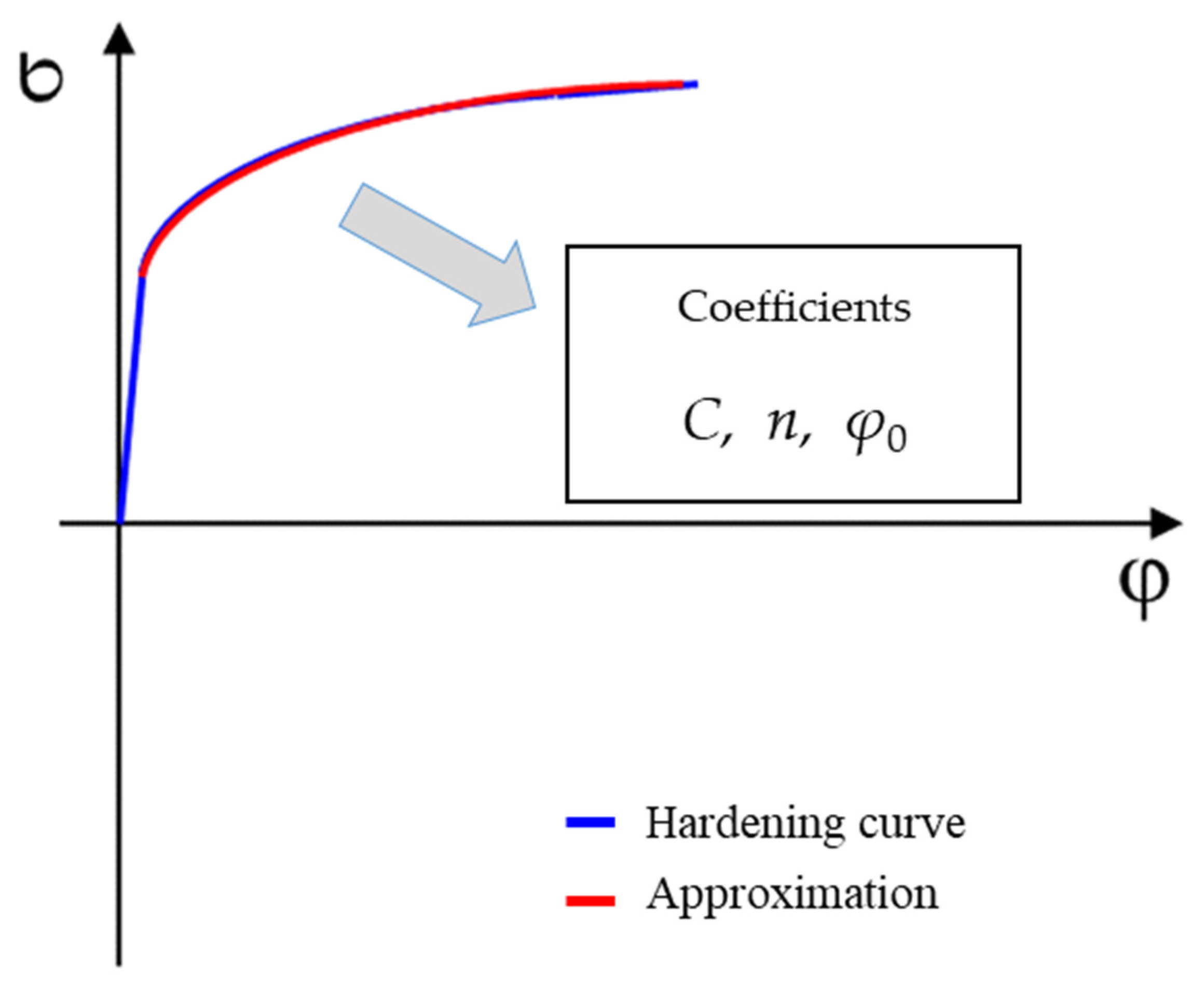
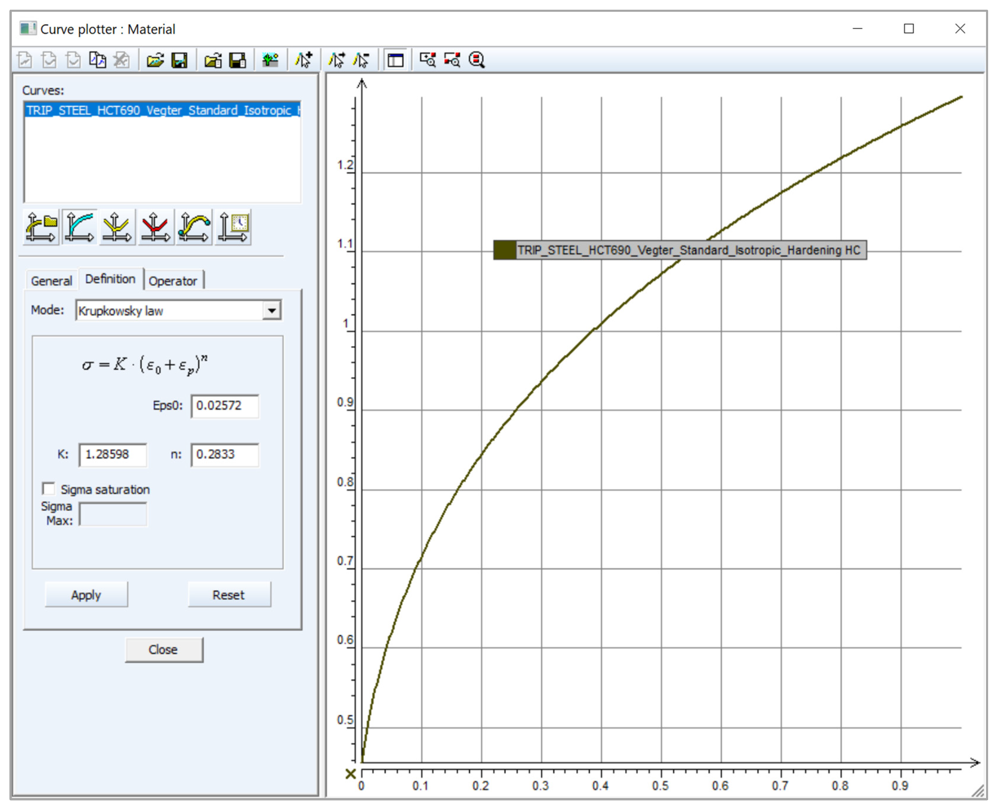
- C—strength coefficient (MPa),
- n—strain hardening exponent (-),
- φ0—offset true strain (-).

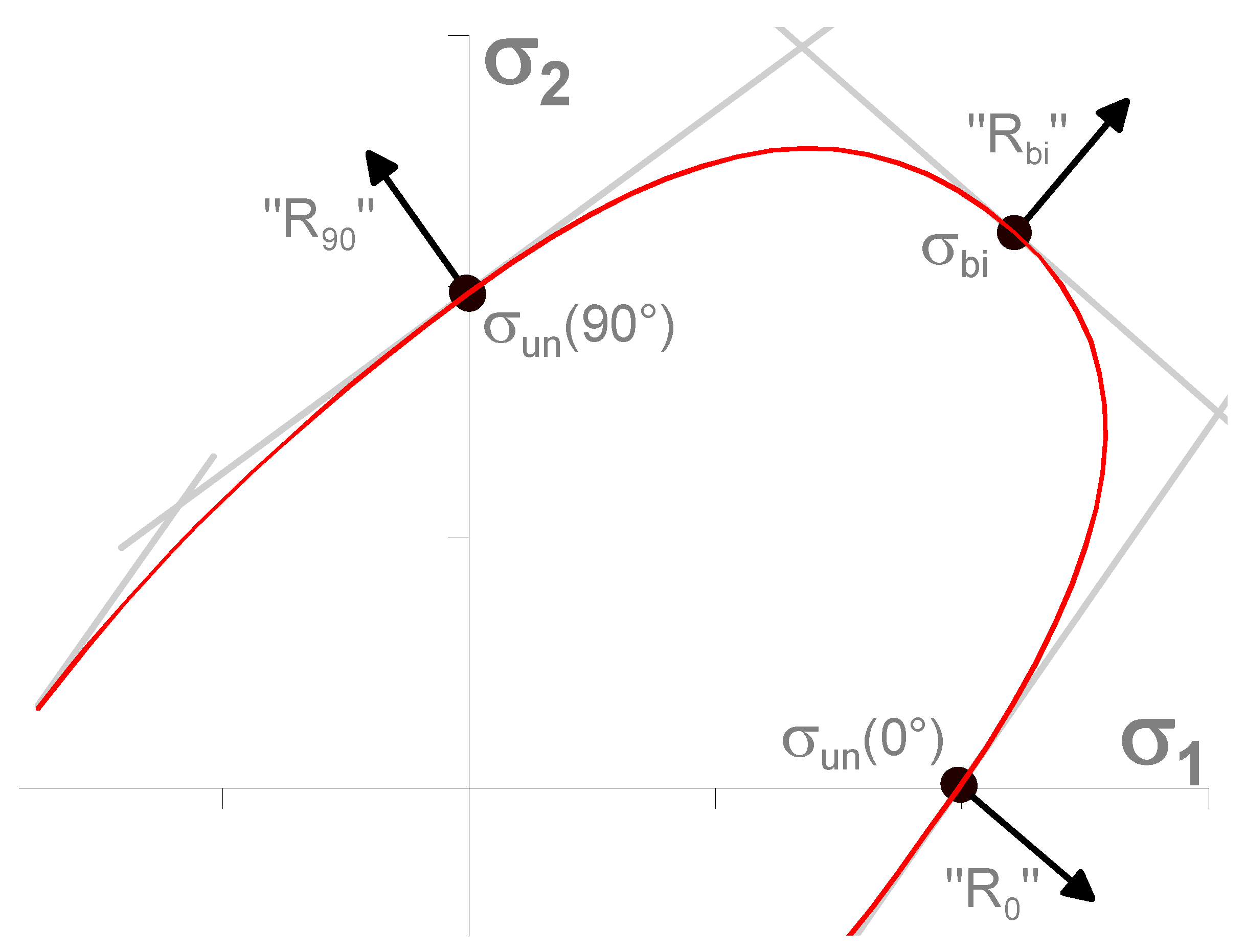
- σ1—principal stress (direction 1) (MPa),
- σ2—principal stress (direction 2) (MPa),
- σxx—stress in the direction 0° (MPa),
- σyy—stress in the direction 90° (MPa),
- σxy—shear stress (MPa),
- ϴ—angle of the coordination system rotation (°).
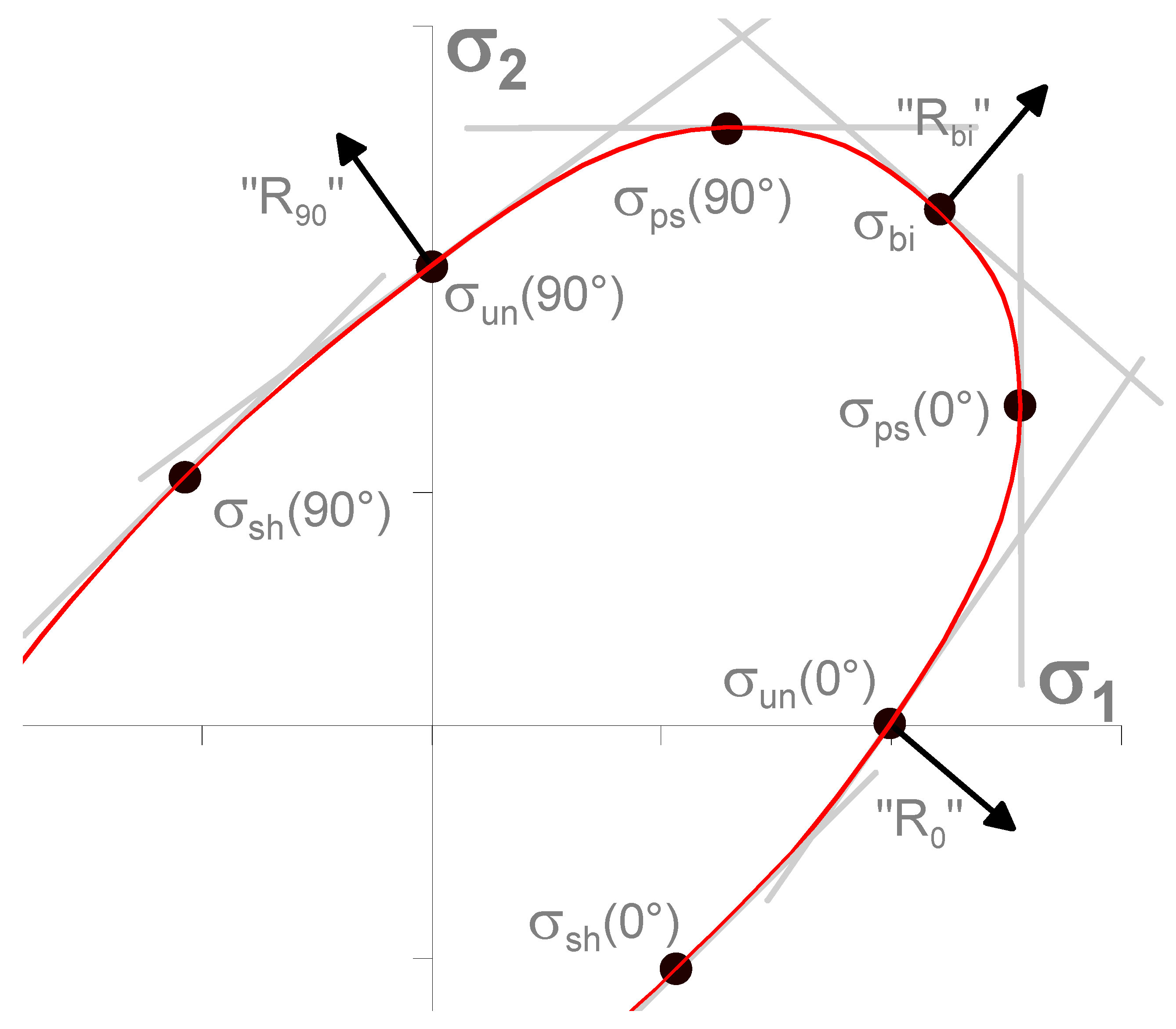
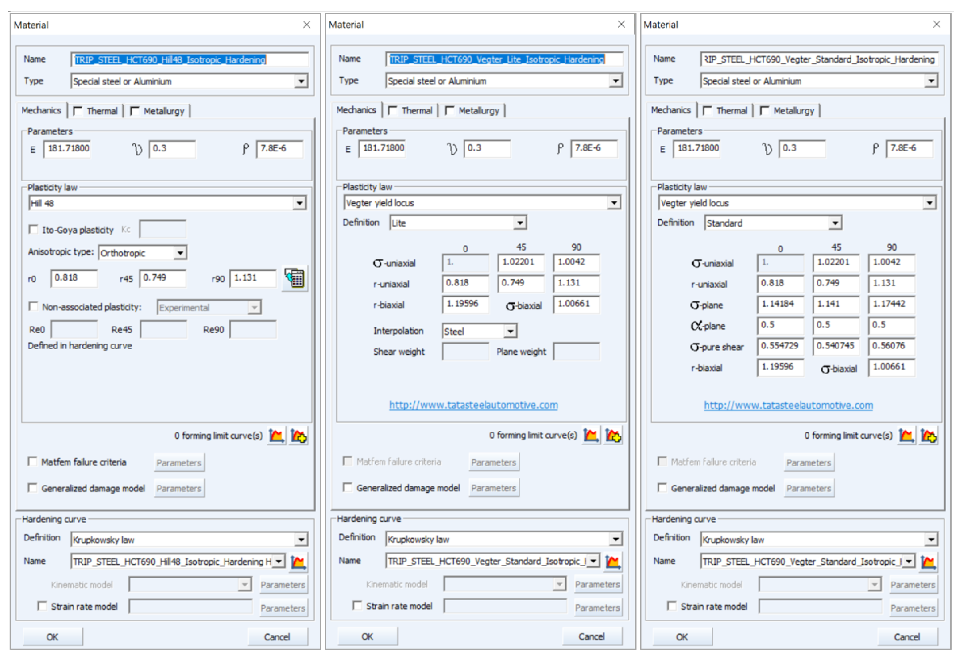
2.3.1. Vegter Lite Yield Criterion
- Young’s modulus E;
- Poisson’s ratio μ;
- Density ρ.
- Static tensile test;
- Hydraulic bulge test.

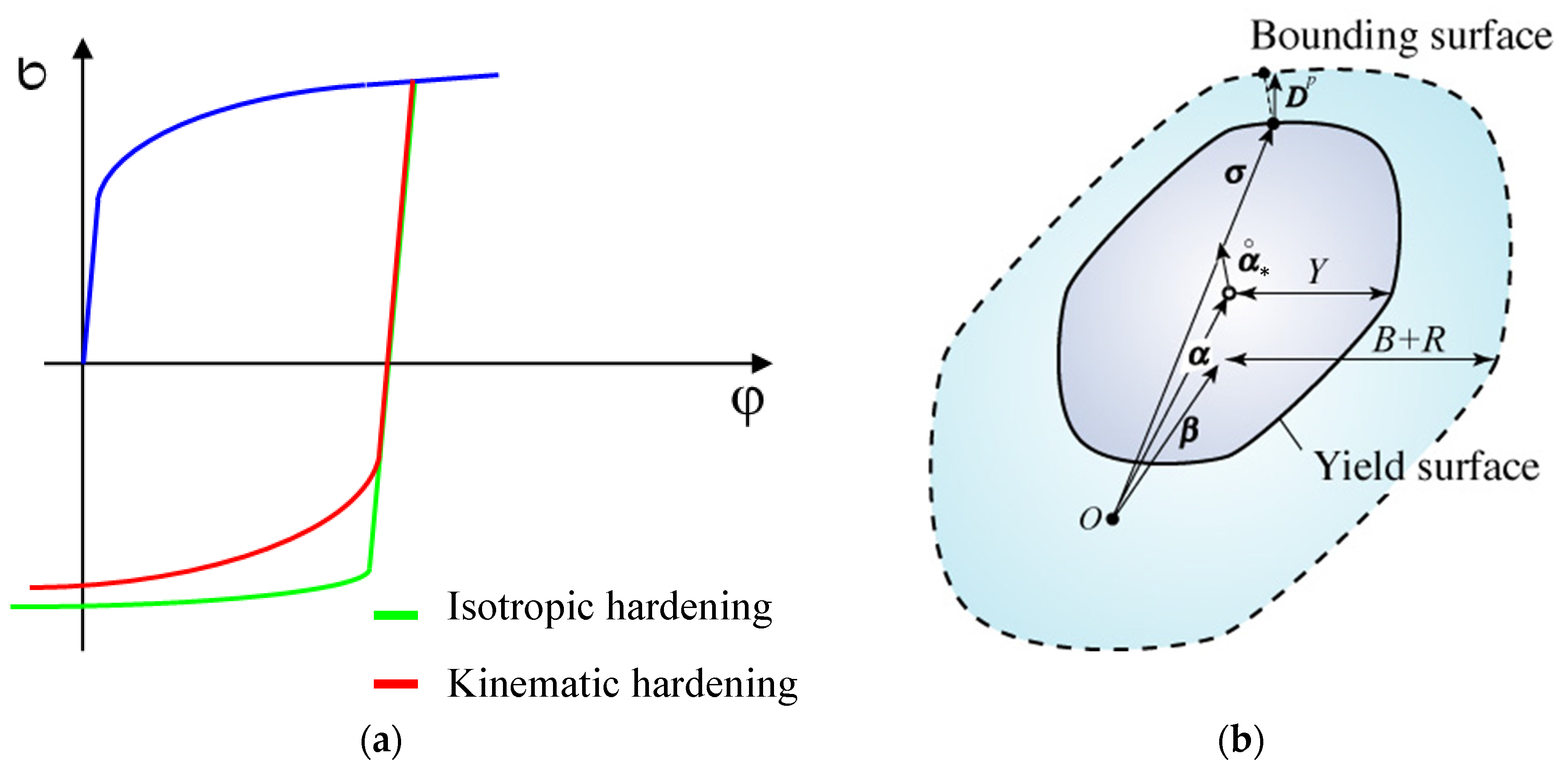
- Isotropic hardening law;
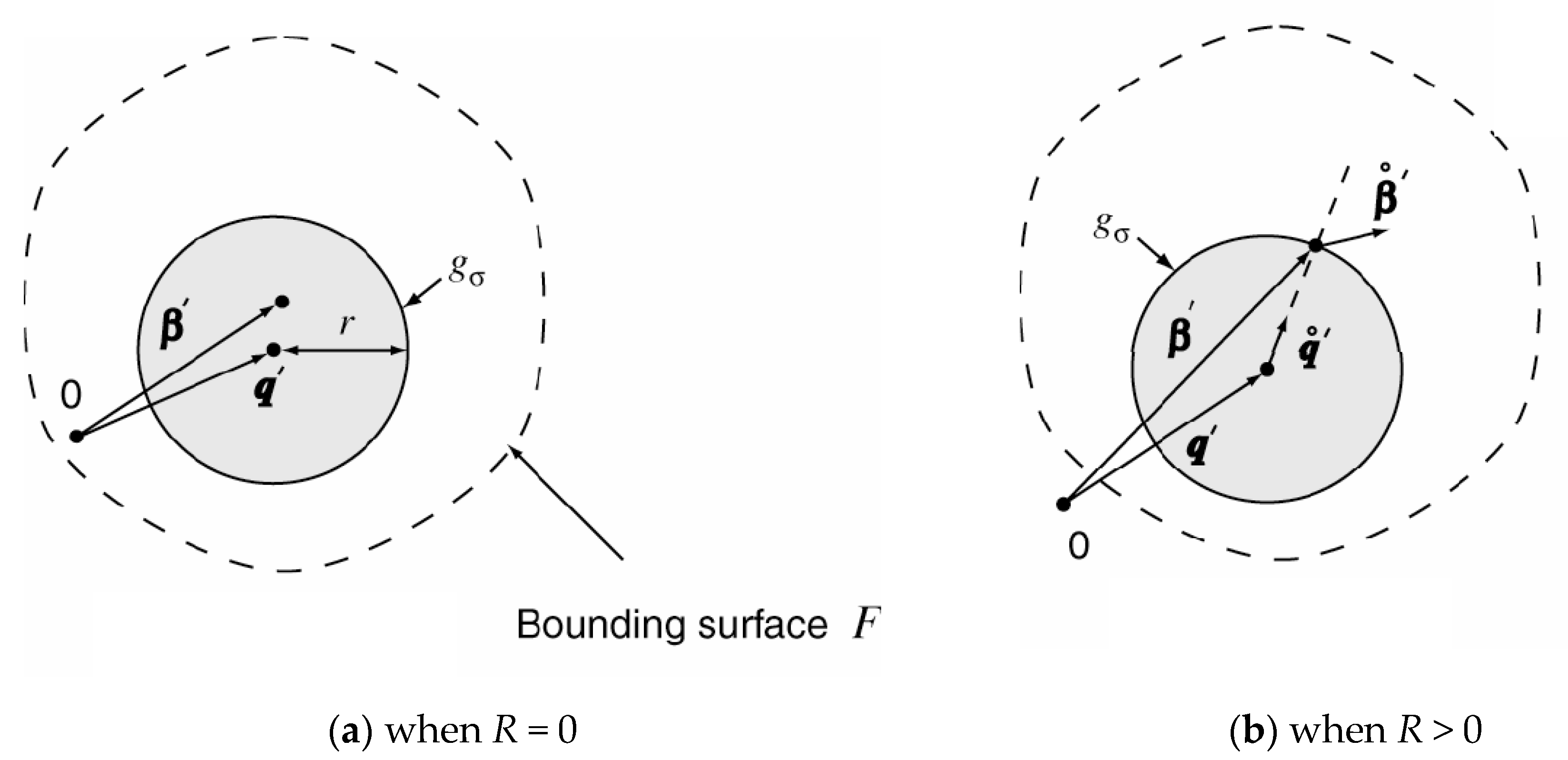
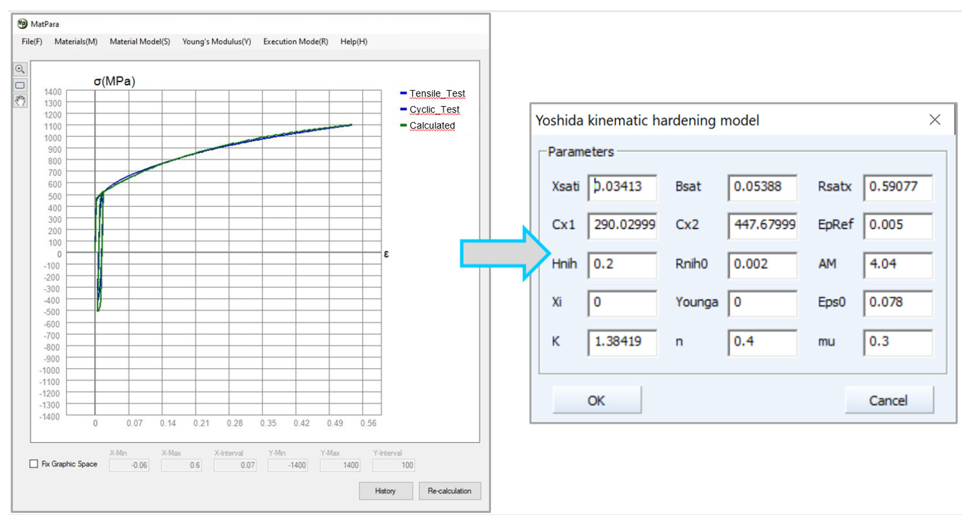
- (Yoshida) Kinematic hardening law.
2.3.2. Vegter Yield Criterion
- Young’s modulus E;
- Poisson’s ratio μ;
- Density ρ.
- Static tensile test;
- Hydraulic bulge test;
- Plane strain tensile test;
- Shear test.

- Isotropic hardening law;
- (Yoshida) Kinematic hardening law.
3. Experimental Part
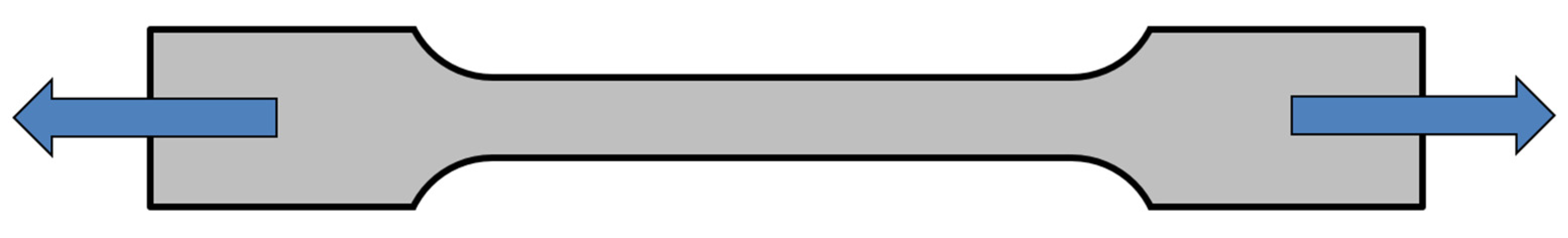
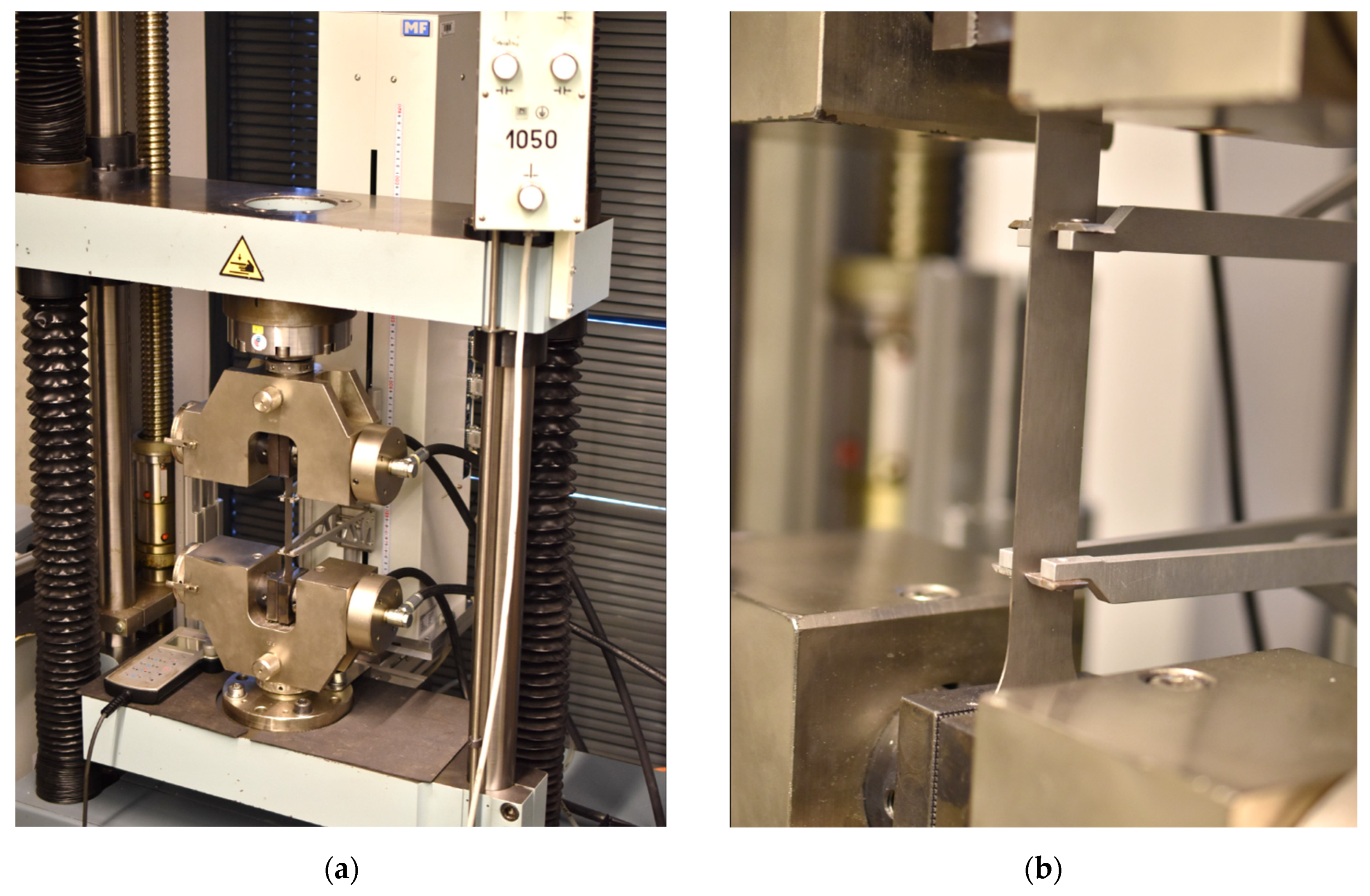
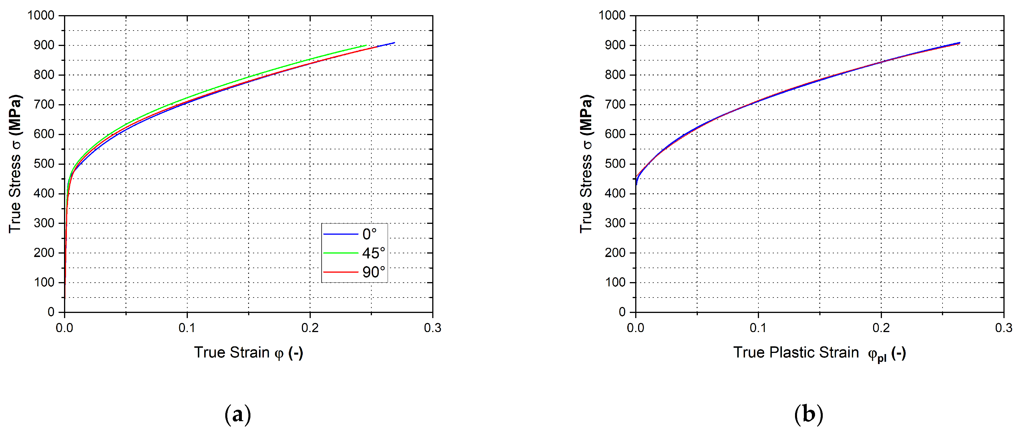
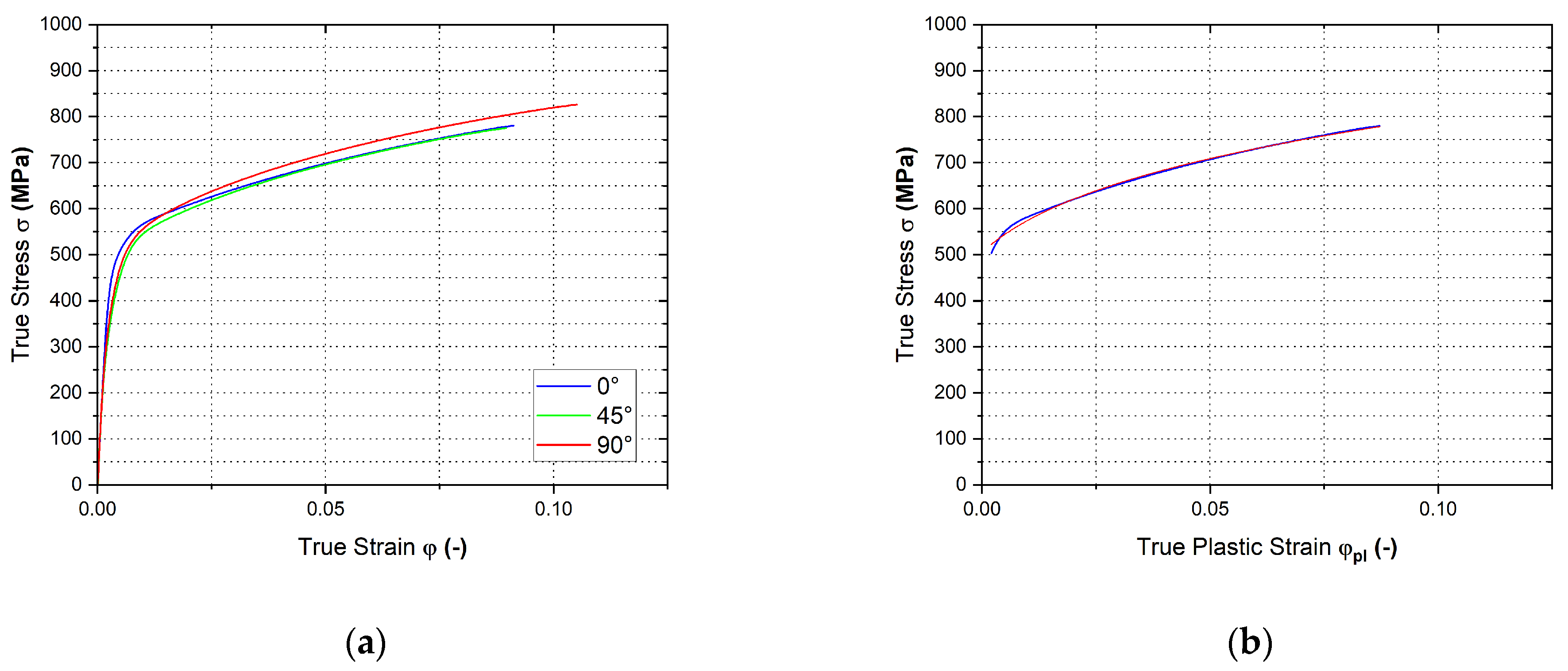
3.1. Static Tensile Test
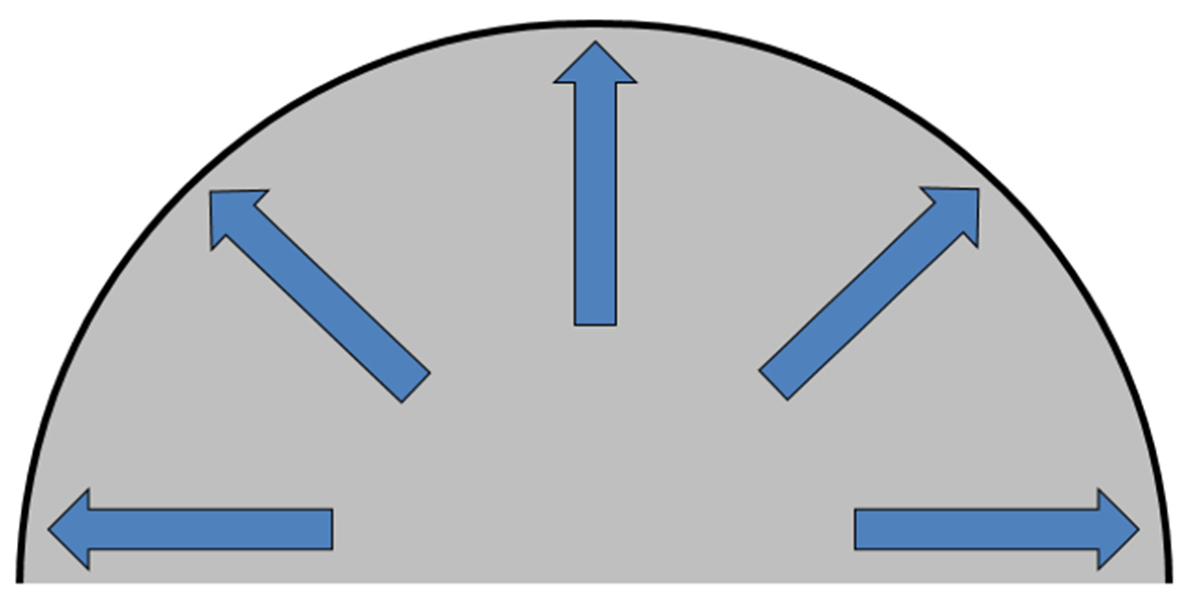
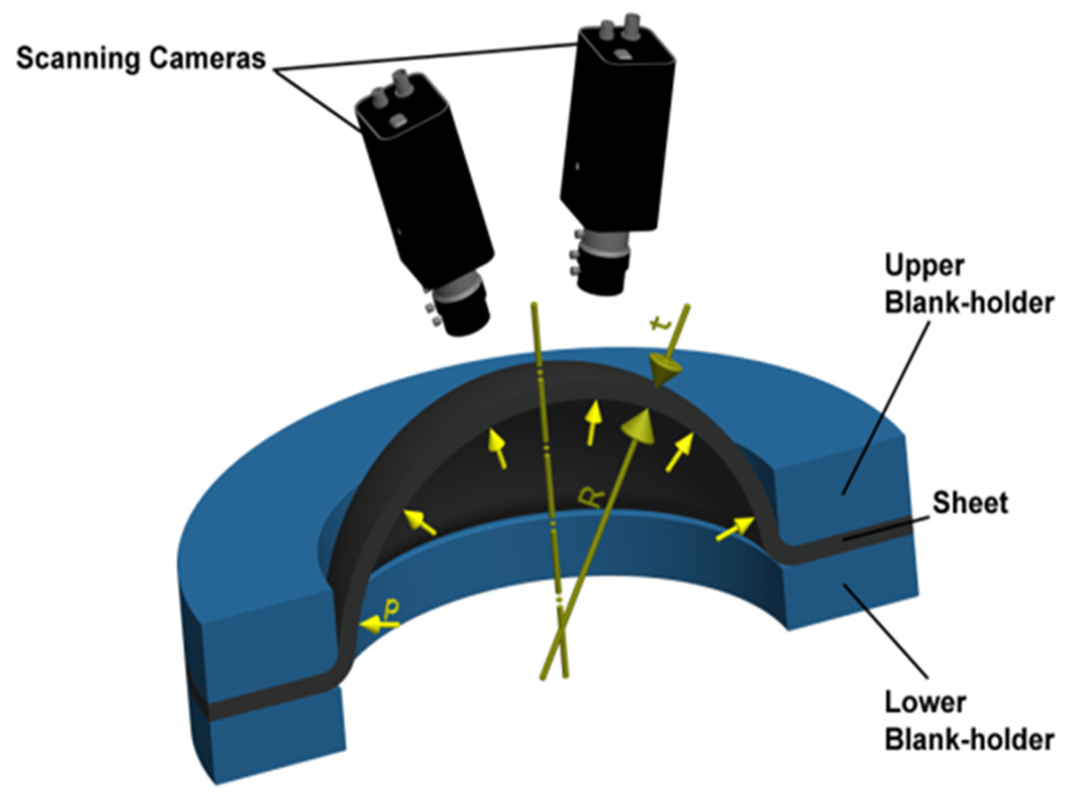
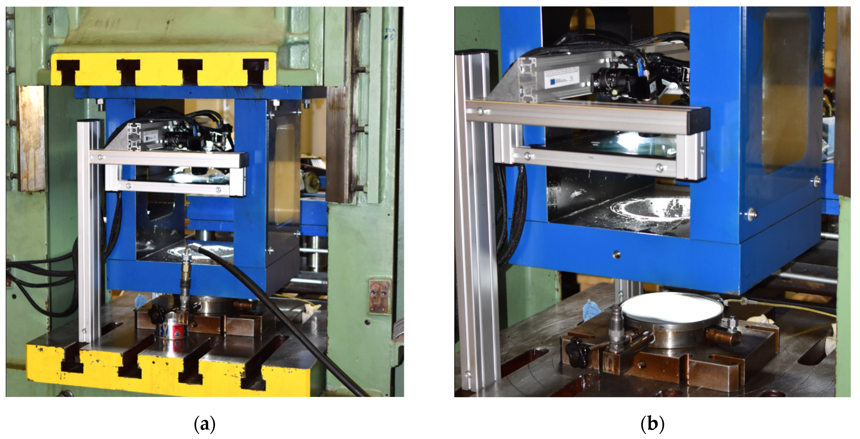
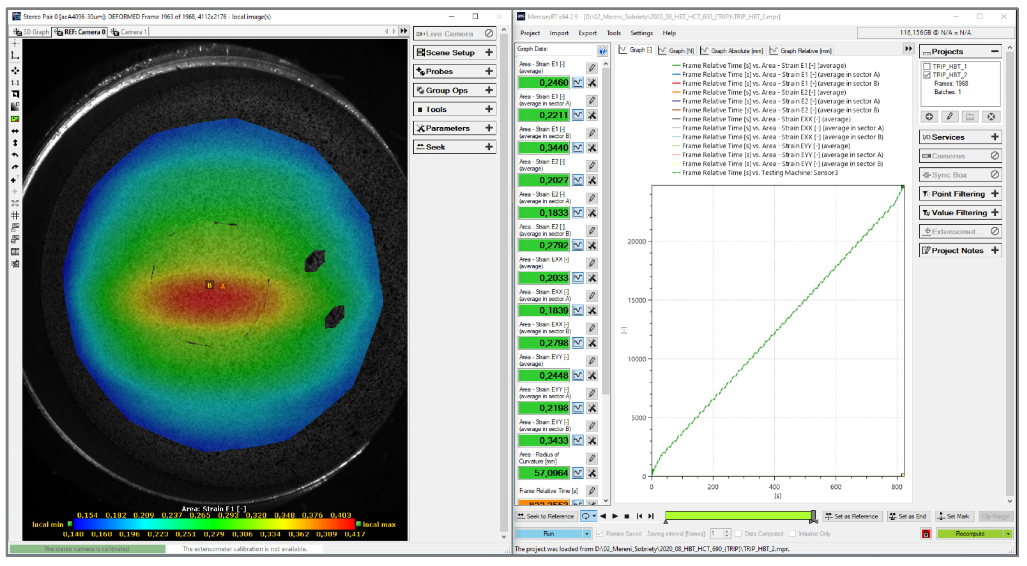
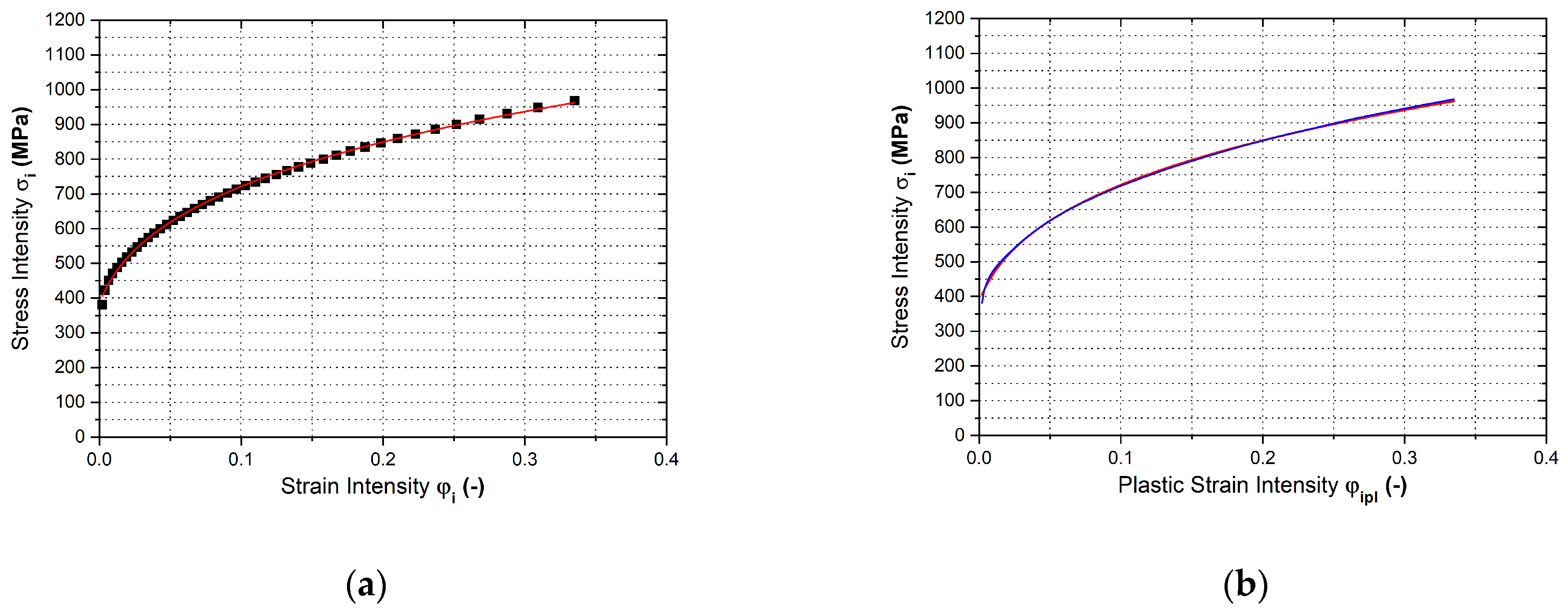
3.2. Hydraulic Bulge Test
- σEF—effective stress [MPa],
- p—hydraulic pressure [MPa],
- φEF—effective strain [-],
- R—radius of curvature [mm],
- φ1,2,3—principal strains [-],
- t, t0—actual and initial thickness [mm].
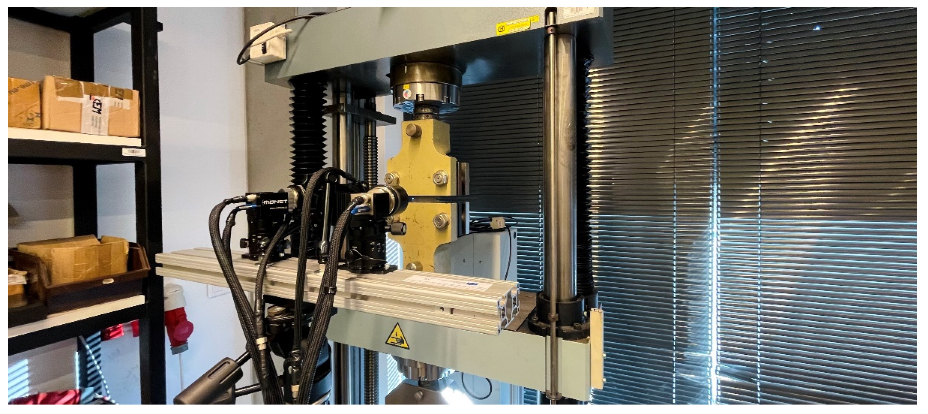
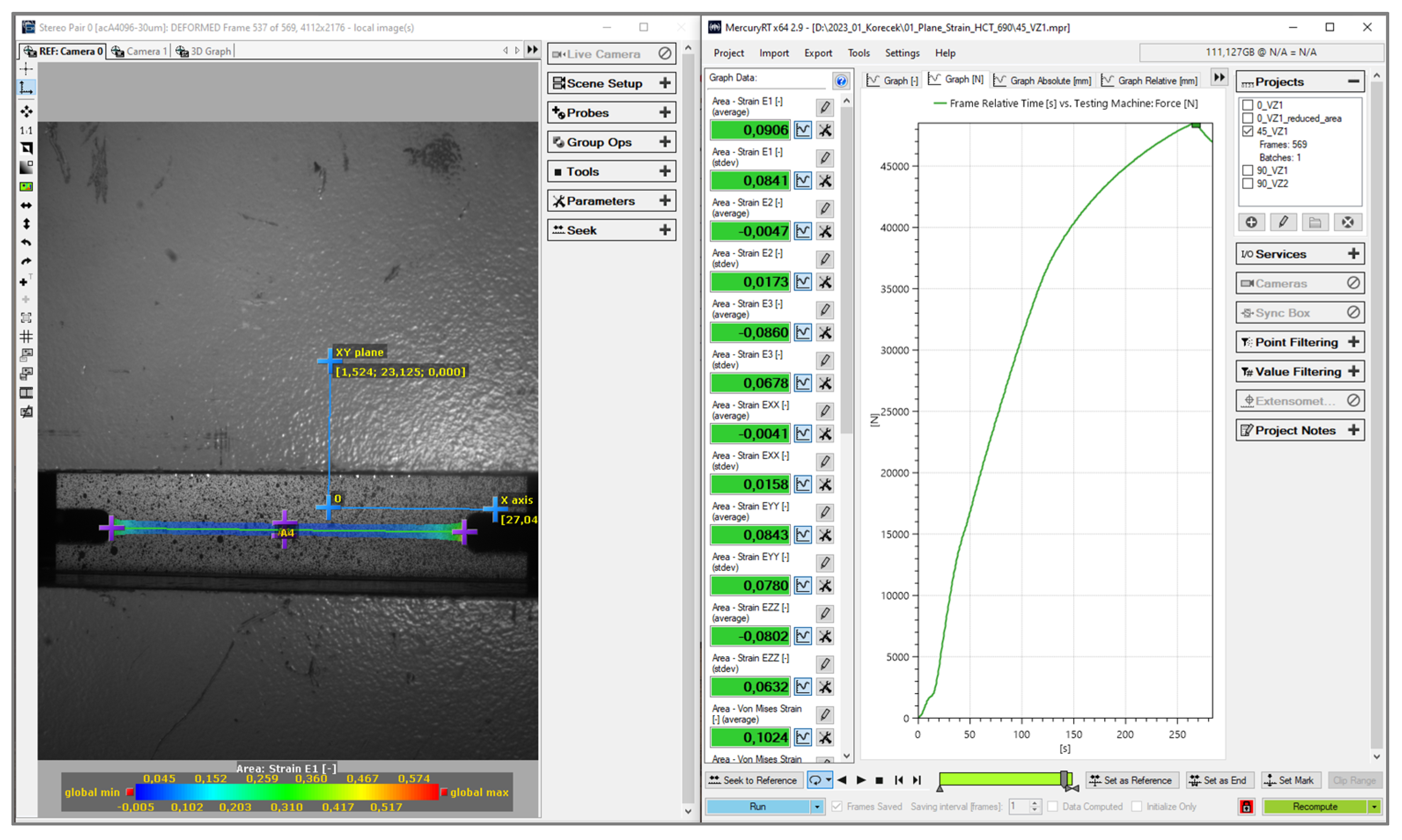
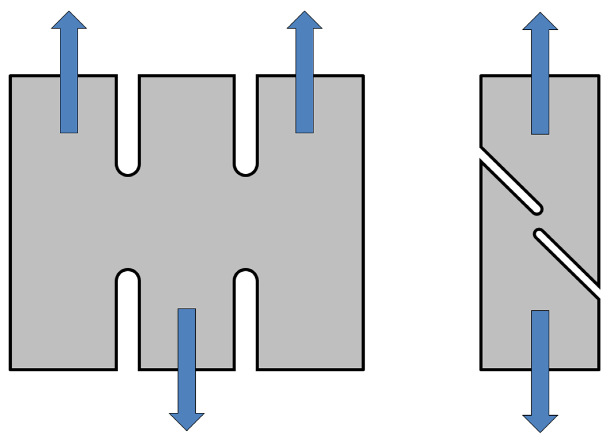
3.3. Plane Strain Test
- φ1—principal strain (length) [-],
- φ2—principal strain (width) [-],
- φ3—principal strain (thickness) [-],
- L—actual length [mm],
- L0—initial length [mm].
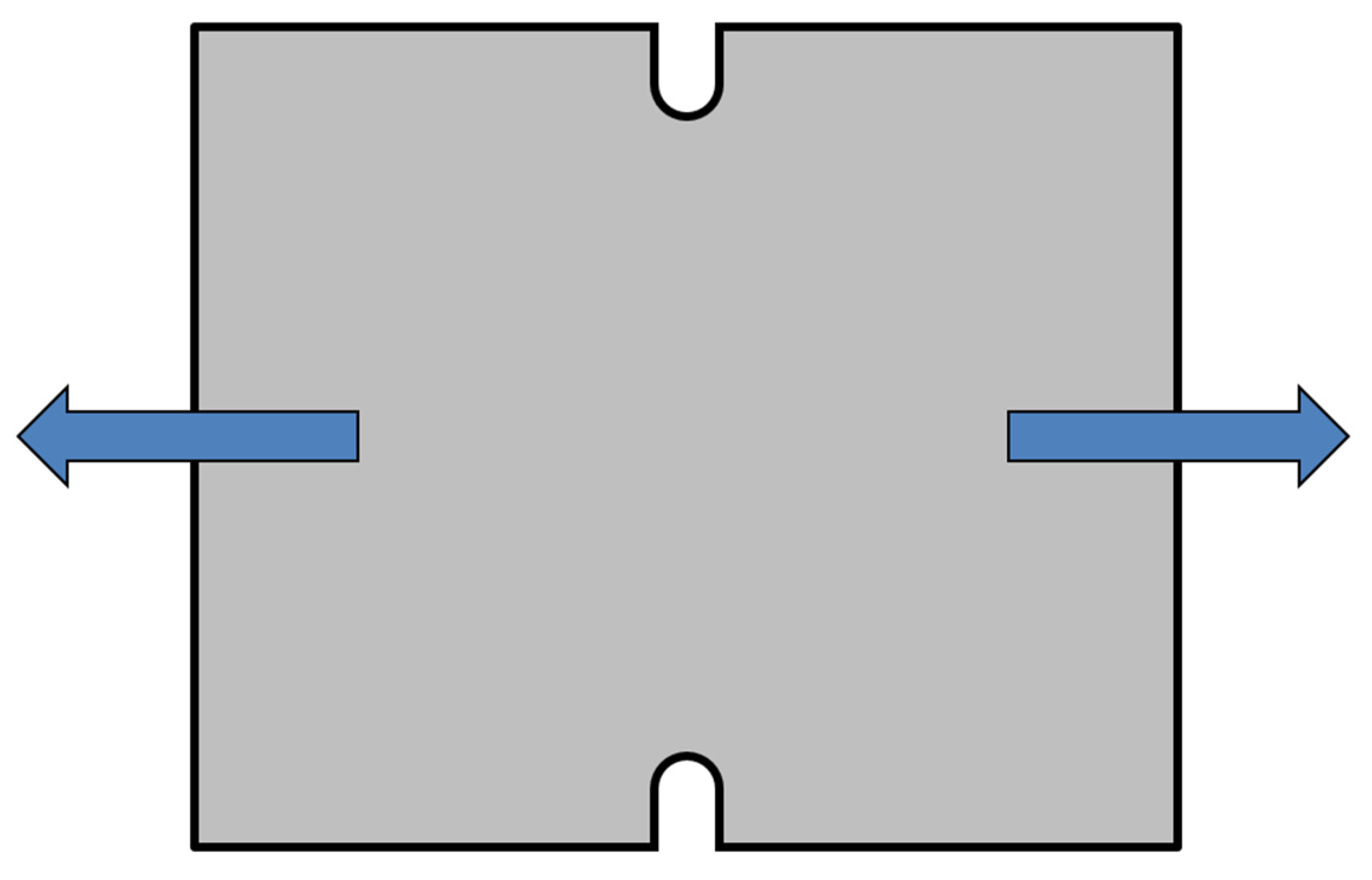
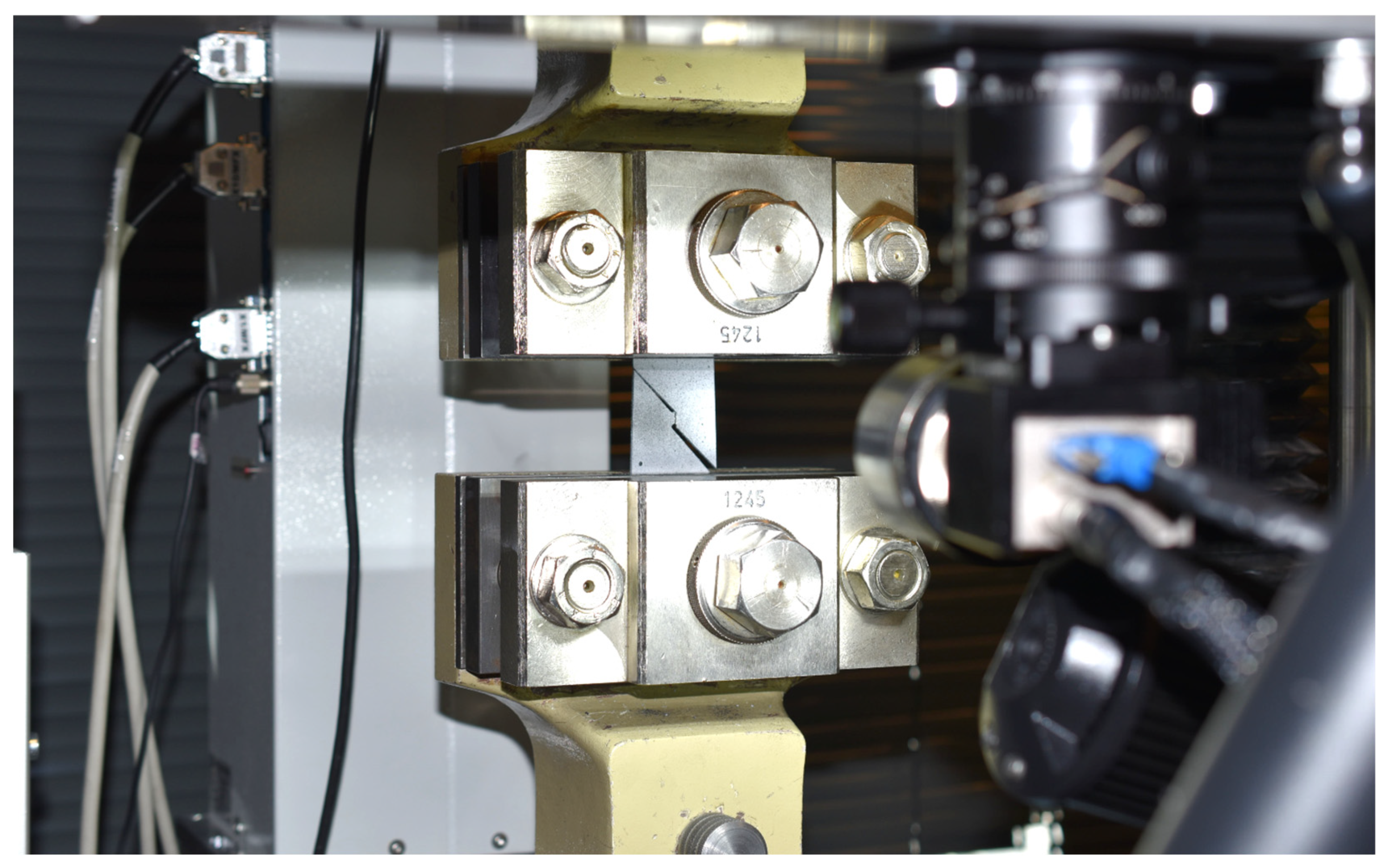
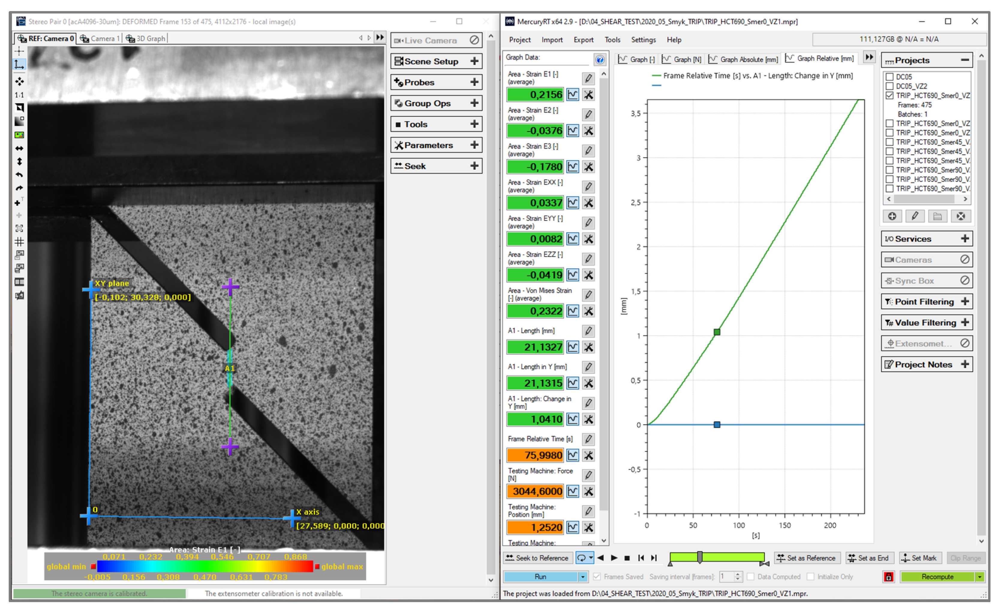
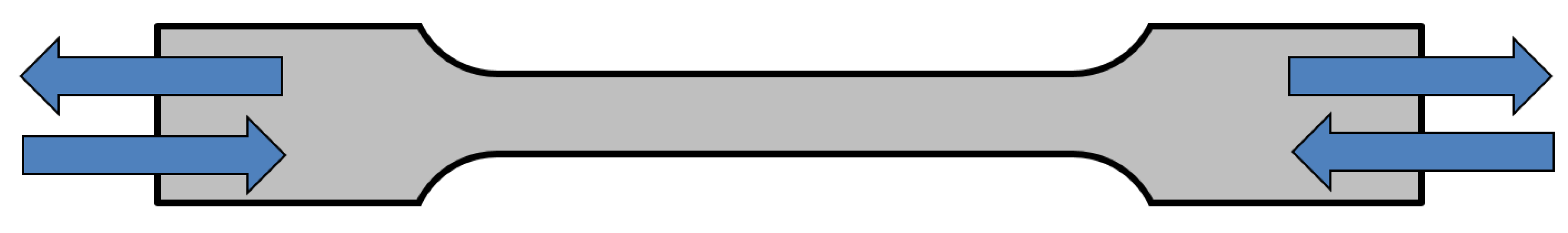
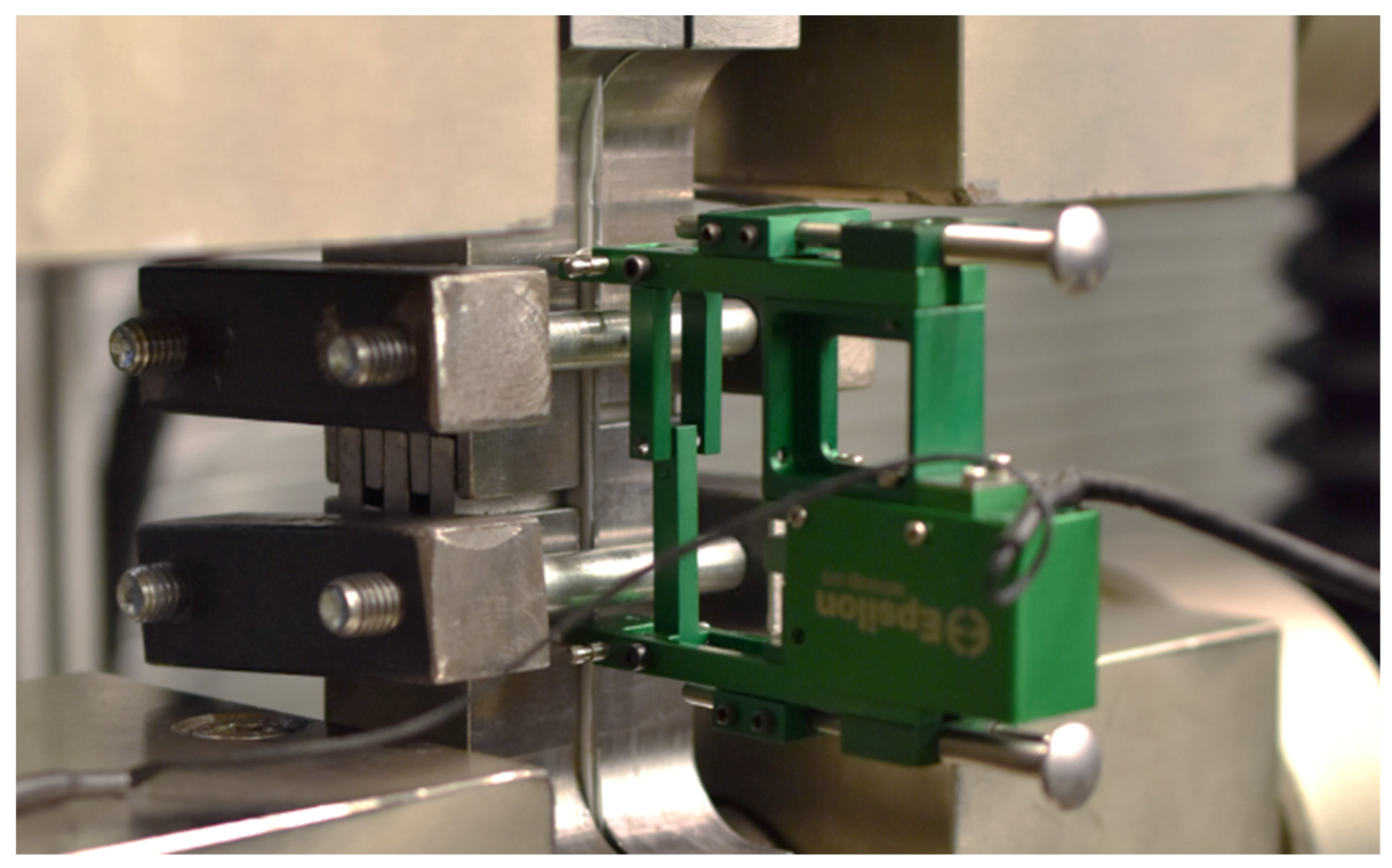
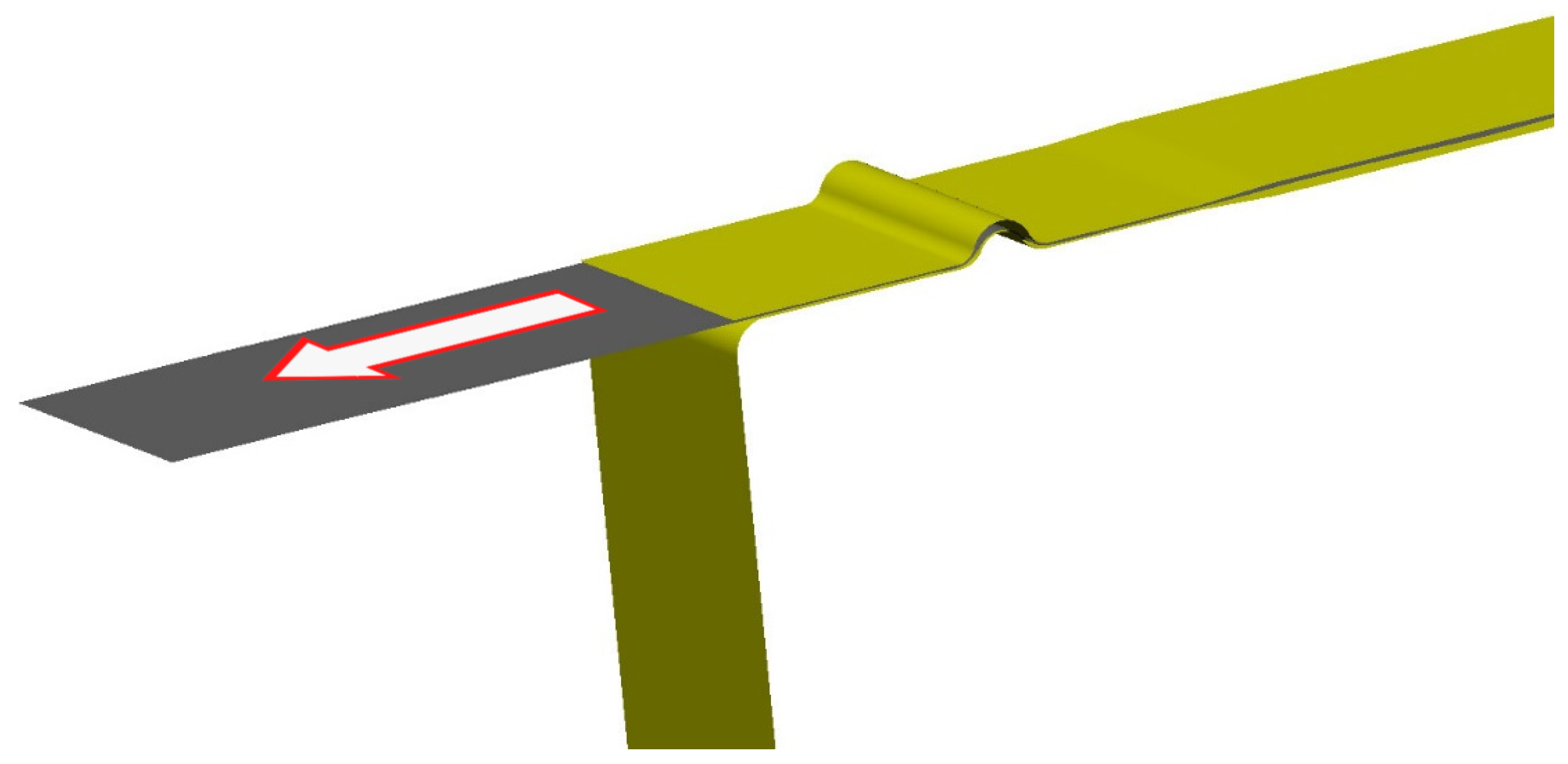
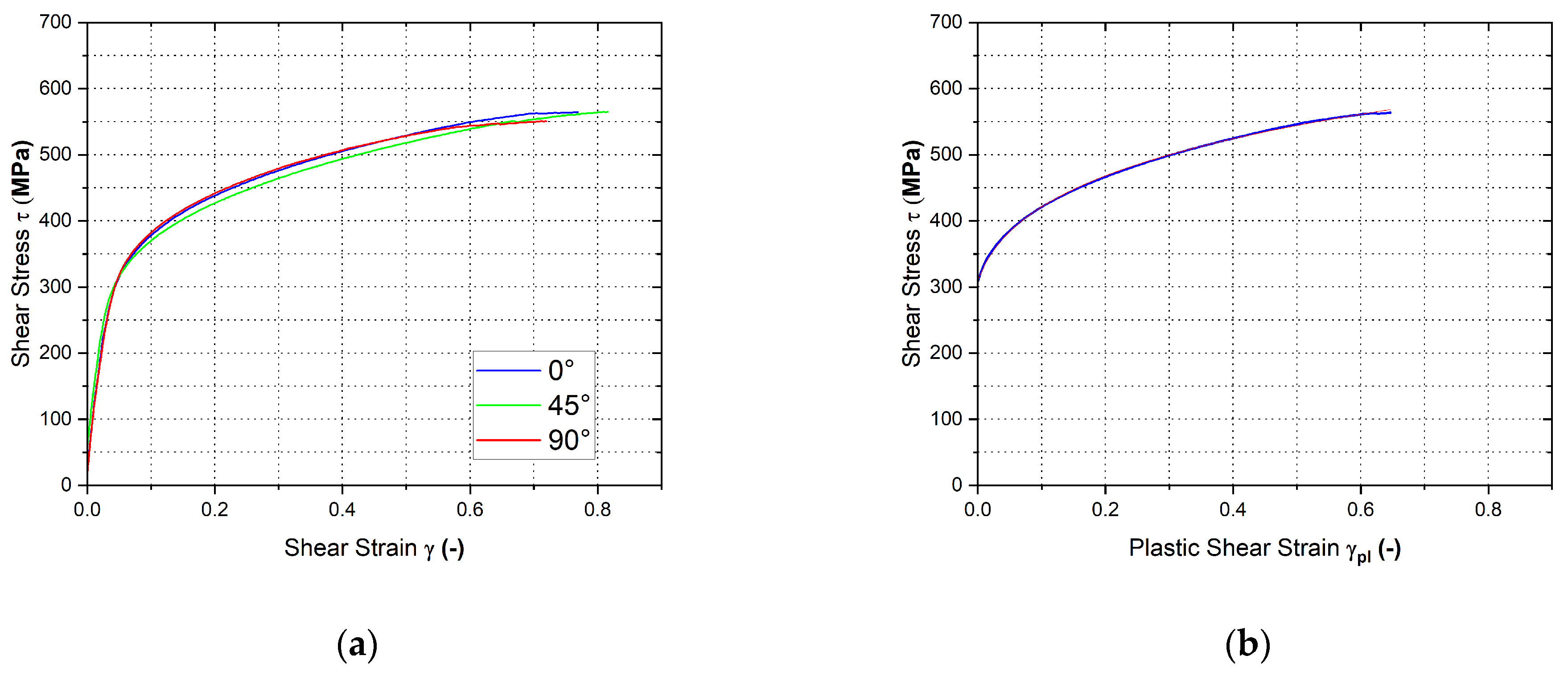
3.4. Shear Test (Slotted Shear Test)
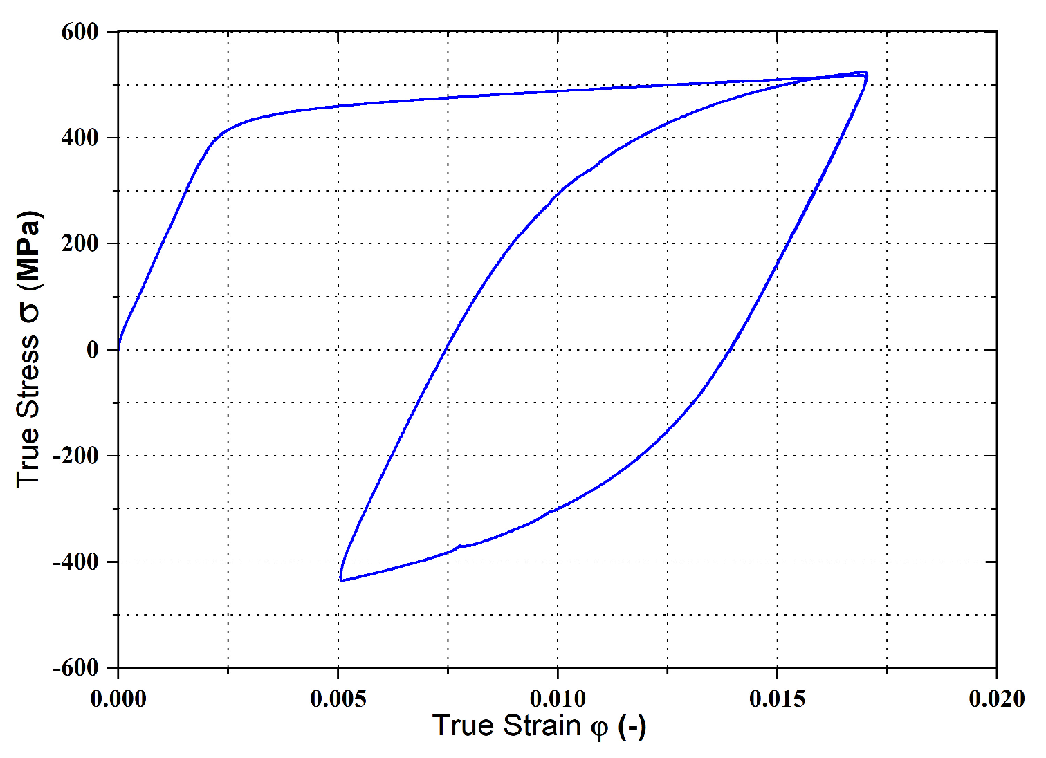
3.5. Cyclic Test (Fully Reversed Alternating Cycle)—Stress Ratio R = −1
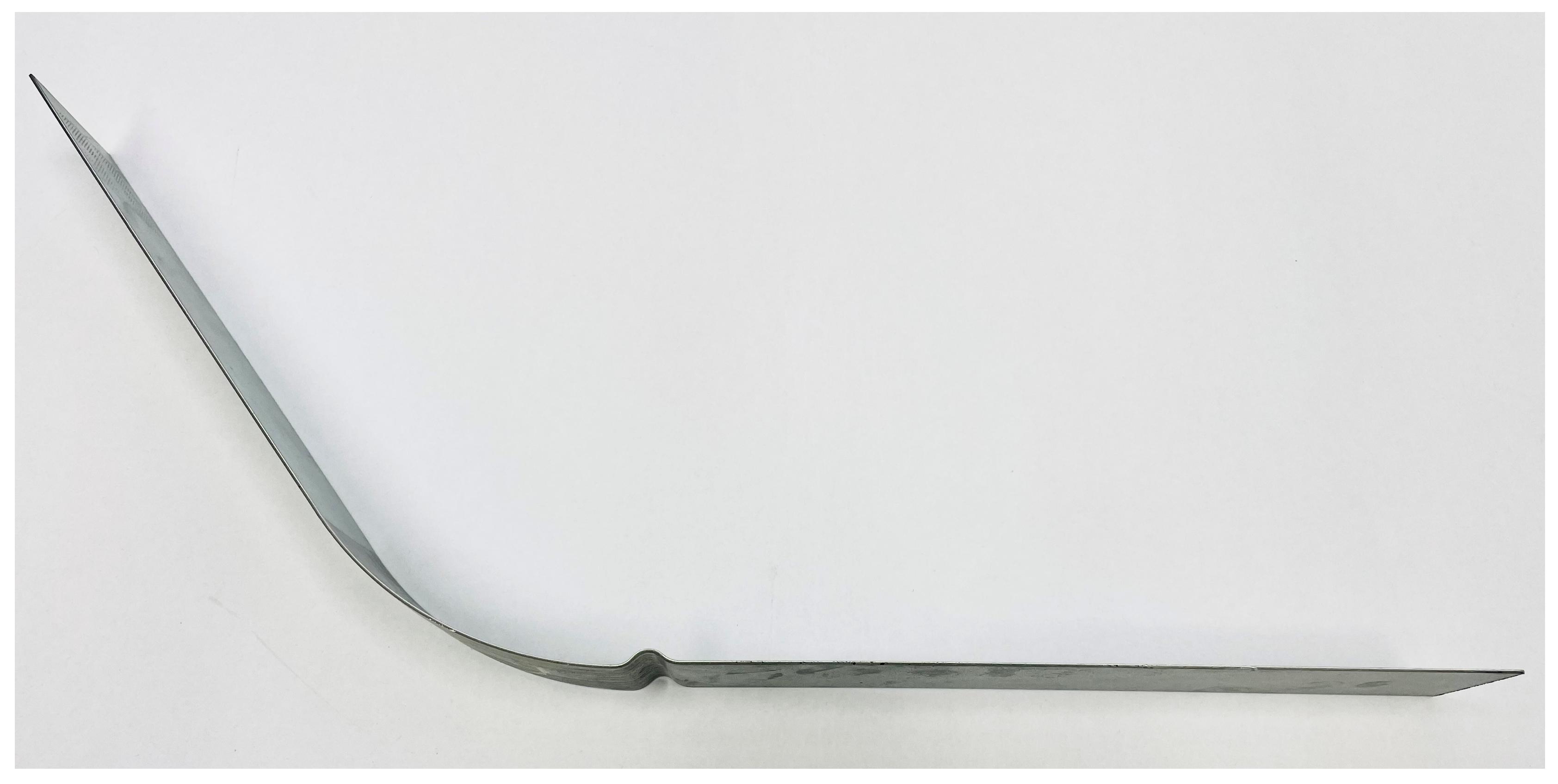
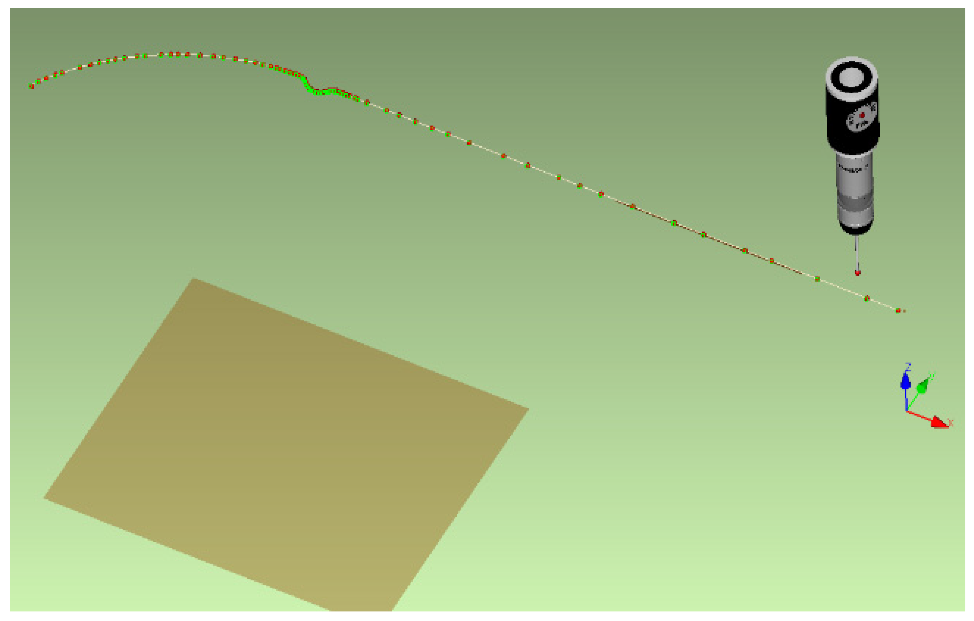
3.6. Preparation of the Real Stamping Corresponding to the Process Set in Numerical Simulation
4. Results
4.1. Mechanical Testing of TRIP Steel HCT690
4.2. Definition of the Used Yield Criteria in the Numerical Simulation Environment of the Software PAM-STAMP 2G
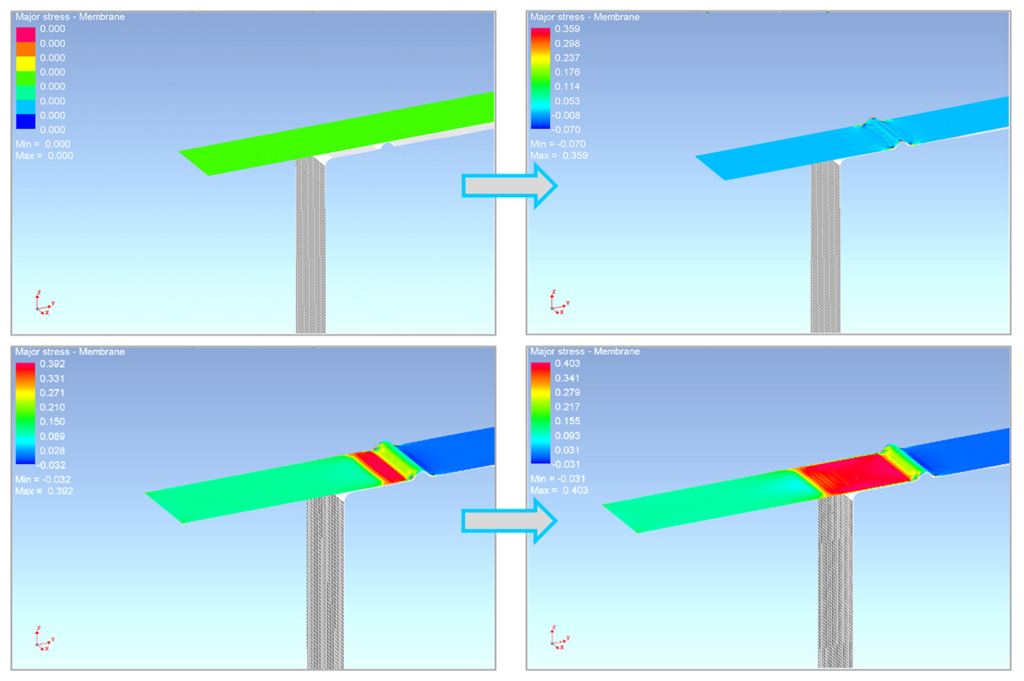
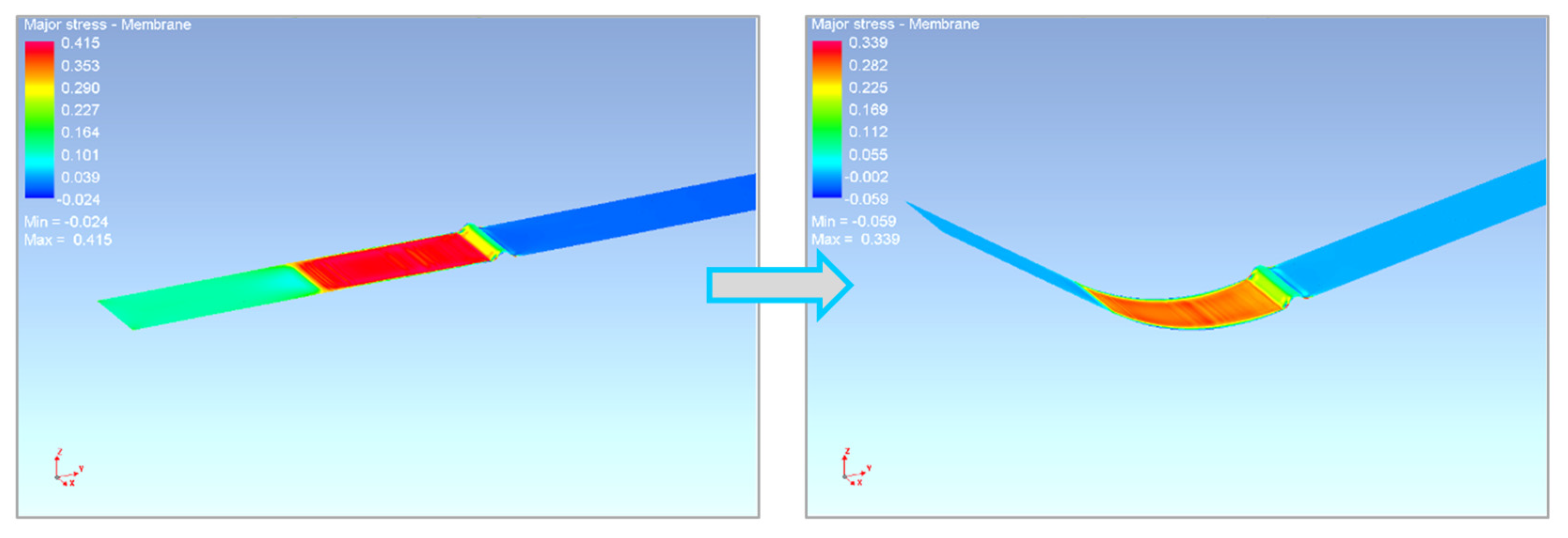
4.3. Numerical Simulation of the Sheet Metal Forming Process
5. Discussion
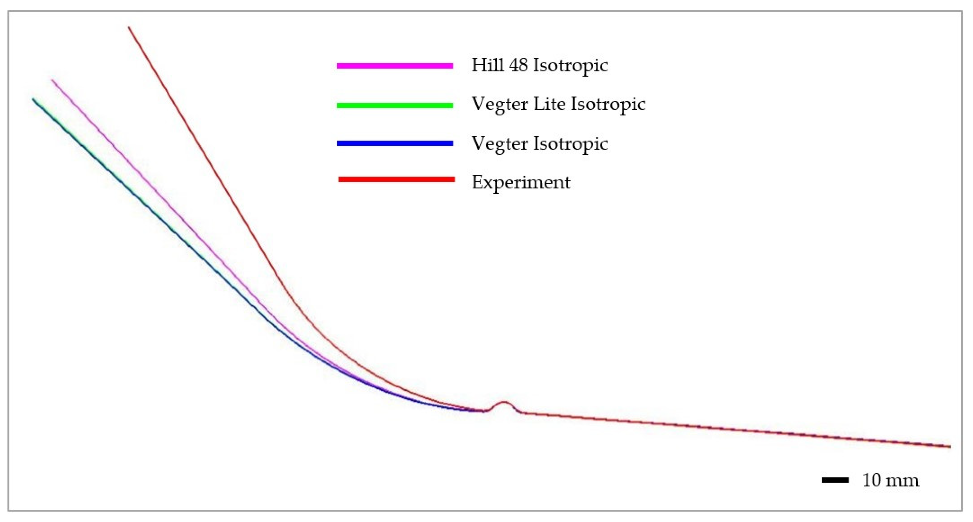
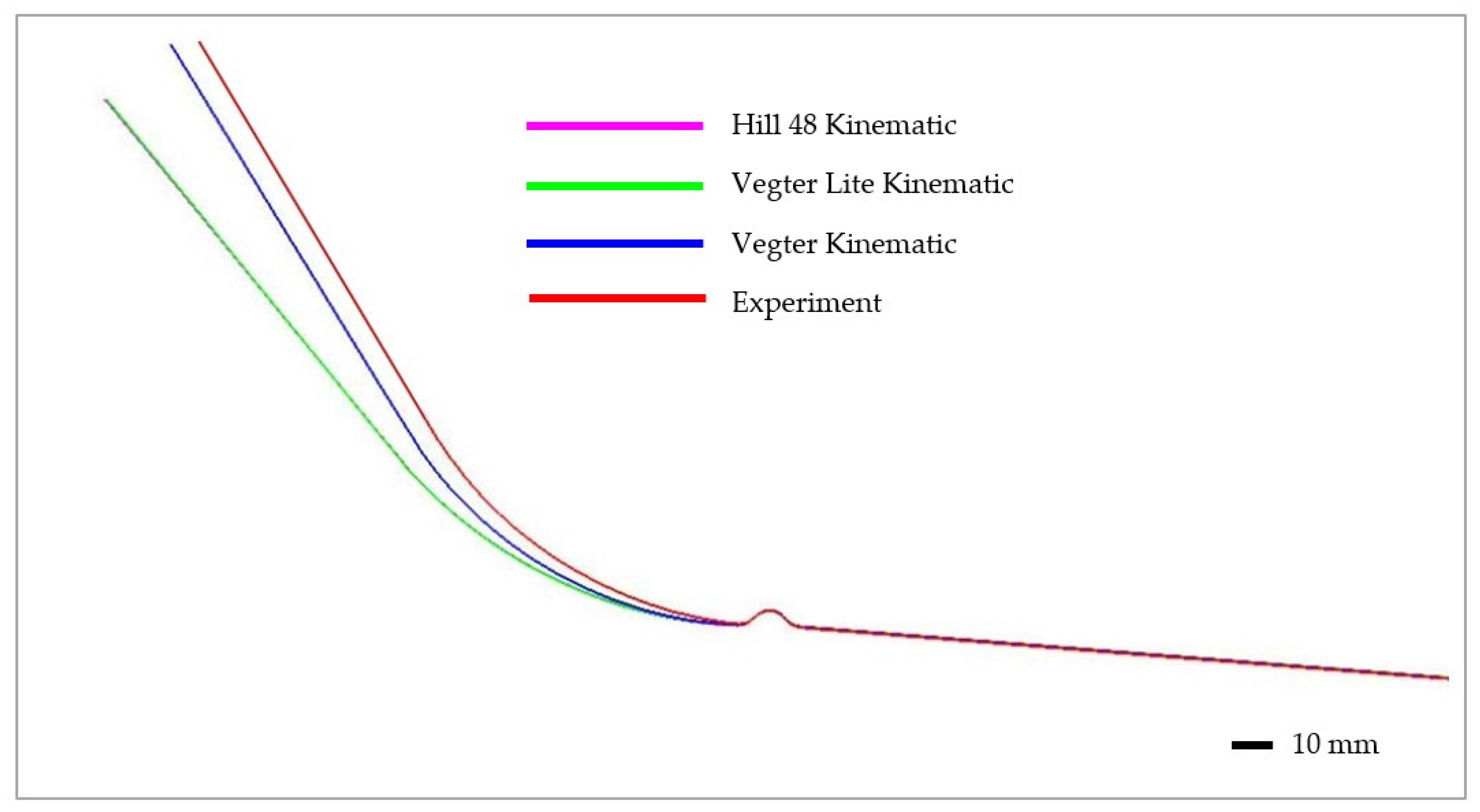
5.1. Comparison of the Yield Criteria Used in the Numerical Simulation
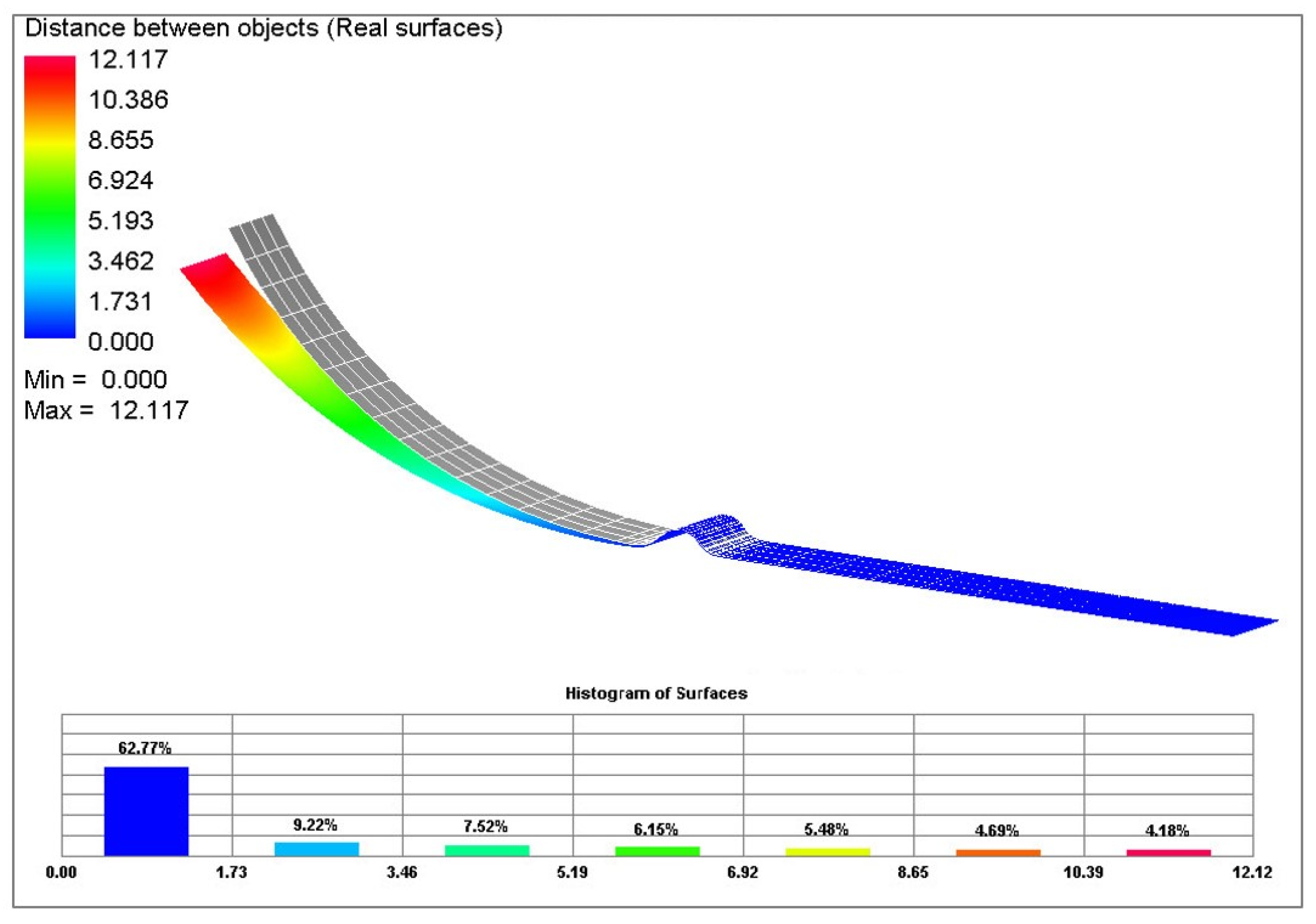
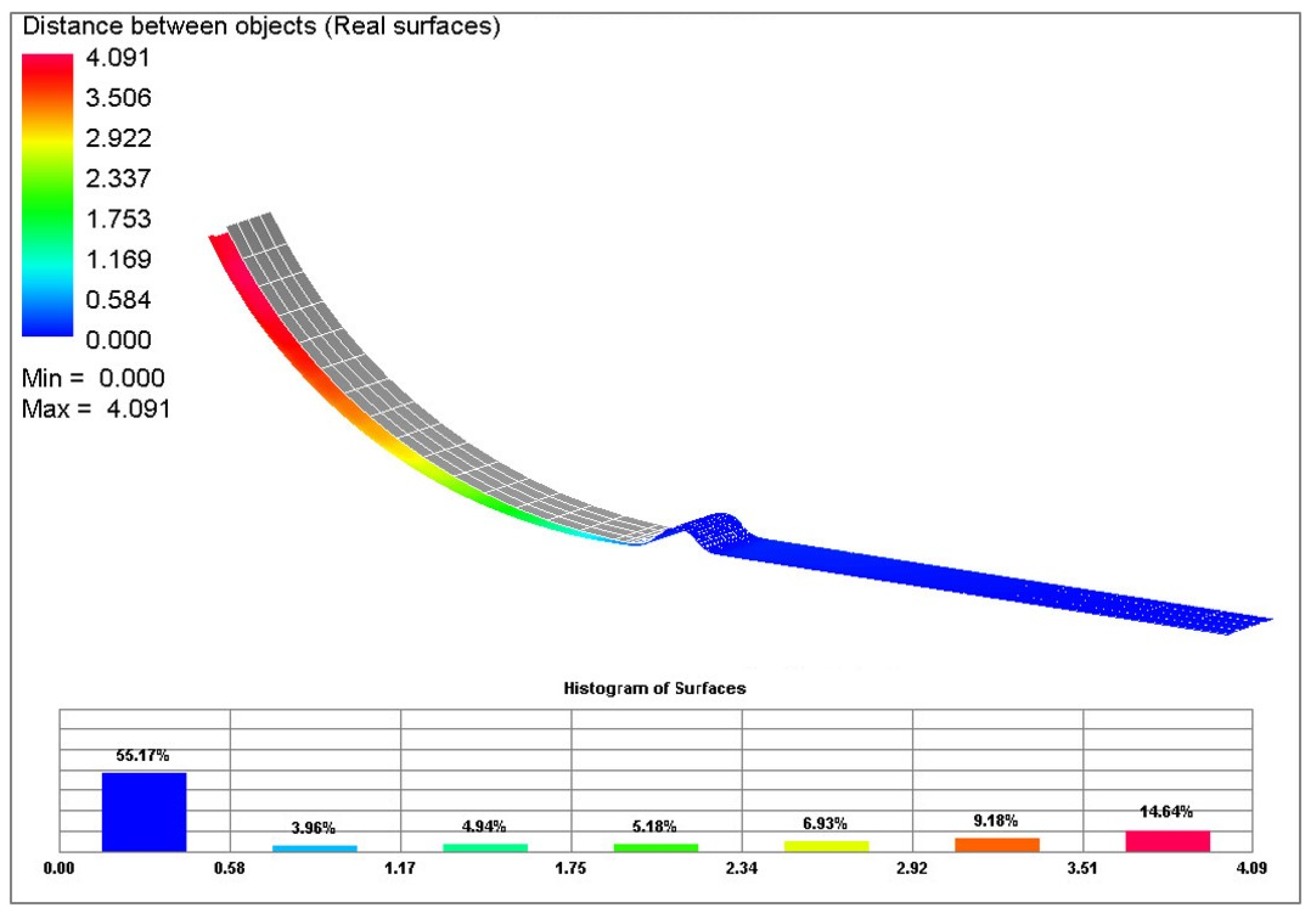
5.2. Comparison of the Results from the Numerical Simulation and the Real Stamping
6. Conclusions
Author Contributions
Funding
Institutional Review Board Statement
Informed Consent Statement
Data Availability Statement
Conflicts of Interest
References
- Rana, R.; Singh, S.B. Automotive Steels: Design, Metallurgy, Processing and Applications; Woodhead Publishing: Cambridge, UK, 2016; ISBN 978-0-08-100653-5. [Google Scholar]
- Abspoel, M.; Scholting, M.E.; Lansbergen, M.; An, Y.; Vegter, H. A New Method for Predicting Advanced Yield Criteria Input Parameters from Mechanical Properties. J. Mater. Process. Technol. 2017, 248, 161–177. [Google Scholar] [CrossRef]
- Vegter, H.; ten Horn, C.; Abspoel, M. The Vegter Lite Material Model: Simplifying Advanced Material Modelling. Int. J. Mater. Form. 2011, 4, 85–92. [Google Scholar] [CrossRef]
- Vegter, H.; Mulder, H.; van Liempt, P.; Heijne, J. Work Hardening Descriptions in Simulation of Sheet Metal Forming Tailored to Material Type and Processing. Int. J. Plast. 2016, 80, 204–221. [Google Scholar] [CrossRef]
- An, Y.G.; Vegter, H. Analytical and Experimental Study of Frictional Behavior in Through-Thickness Compression Test. J. Mater. Process. Technol. 2005, 160, 148–155. [Google Scholar] [CrossRef]
- Kok, P.J.J.; Spanjer, W.; Vegter, H. A Microstructure Based Model for the Mechanical Behavior of Multiphase Steels. Key Eng. Mater. 2015, 651–653, 975–980. [Google Scholar] [CrossRef]
- An, Y.G.; Vegter, H.; Elliott, L. A Novel and Simple Method for the Measurement of Plane Strain Work Hardening. J. Mater. Process. Technol. 2004, 155–156, 1616–1622. [Google Scholar] [CrossRef]
- Hu, Q.; Yoon, J.W.; Manopulo, N.; Hora, P. A Coupled Yield Criterion for Anisotropic Hardening with Analytical Description under Associated Flow Rule: Modeling and Validation. Int. J. Plast. 2021, 136, 102882. [Google Scholar] [CrossRef]
- Komischke, T.; Hora, P.; Domani, G. A New Experimental Method for the Evaluation of Fracture Criteria in Bulk Forming Operations. In Experimental and Numerical Methods in the FEM Based Crack Prediction; Institute of Virtual Manufacturing, ETH Zurich: Zurich, Switzerland, 2018; pp. 65–69. [Google Scholar]
- Raemy, C.; Manopulo, N.; Hora, P. On the Modelling of Plastic Anisotropy, Asymmetry and Directional Hardening of Commercially Pure Titanium: A Planar Fourier Series Based Approach. Int. J. Plast. 2017, 91, 182–204. [Google Scholar] [CrossRef]
- Hippke, H.; Hirsiger, S.; Rudow, F.; Berisha, B.; Hora, P. Optimized Prediction of Strain Distribution with Crystal Plasticity Supported Definition of Yielding Direction; ETH Zurich, Institute of Virtual Manufacturing: Zurich, Switzerland, 2019. [Google Scholar]
- Harsch, D.; Heingärtner, J.; Hortig, D.; Hora, P. Process Windows for Sheet Metal Parts Based on Metamodels. J. Phys. Conf. Ser. 2016, 734, 032014. [Google Scholar] [CrossRef]
- Hora, P.; Tong, L.; Gorji, M.; Manopulo, N.; Berisha, B. Significance of the Local Sheet Curvature in the Prediction of Sheet Metal Forming Limits by Necking Instabilities and Cracks. In Proceedings of the NUMIFORM 2016: The 12th International Conference on Numerical Methods in Industrial Forming Processes, EDP Sciences, Troyes, France, 4–7 July 2016; Volume 80, p. 11003. [Google Scholar]
- Yoshida, F.; Uemori, T. Cyclic Plasticity Model for Accurate Simulation of Springback of Sheet Metals. In 60 Excellent Inventions in Metal Forming; Tekkaya, A.E., Homberg, W., Brosius, A., Eds.; Springer: Berlin/Heidelberg, Germany, 2015; pp. 61–66. ISBN 978-3-662-46312-3. [Google Scholar]
- Yoshida, F.; Hamasaki, H.; Uemori, T. A Model of Anisotropy Evolution of Sheet Metals. Procedia Eng. 2014, 81, 1216–1221. [Google Scholar] [CrossRef]
- Uemori, T.; Sumikawa, S.; Naka, T.; Ma, N.; Yoshida, F. Influence of Bauschinger Effect and Anisotropy on Springback of Aluminum Alloy Sheets. Keikinzoku J. Jpn. Inst. Light Met. 2015, 65, 582–587. [Google Scholar] [CrossRef][Green Version]
- Tada, N.; Uemori, T. Microscopic Elastic and Plastic Inhomogeneous Deformations and Height Changes on the Surface of a Polycrystalline Pure-Titanium Plate Specimen under Cyclic Tension. Appl. Sci. 2018, 8, 1907. [Google Scholar] [CrossRef]
- Yoshida, F.; Hamasaki, H.; Uemori, T. Modeling of Anisotropic Hardening of Sheet Metals Including Description of the Bauschinger Effect. Int. J. Plast. 2015, 75, 170–188. [Google Scholar] [CrossRef]
- Uemori, T.; Naka, T.; Tada, N.; Yoshimura, H.; Katahira, T.; Yoshida, F. Theoretical Predictions of Fracture and Springback for High Tensile Strength Steel Sheets under Stretch Bending. Procedia Eng. 2017, 207, 1594–1598. [Google Scholar] [CrossRef]
- Yoshida, F. Description of Elastic–Plastic Stress–Strain Transition in Cyclic Plasticity and Its Effect on Springback Prediction. Int. J. Mater. Form. 2022, 15, 12. [Google Scholar] [CrossRef]
- Yoshida, F. Elasto-Plasticity Models for Accurate Metal Forming Simulation II: Role of Accurate Material Model in Springback Simulation. Zair. J. Soc. Mater. Sci. Jpn. 2023, 72, 144–149. [Google Scholar] [CrossRef]
- Yoshida, F. Elasto-Plasticity Models for Accurate Metal Forming Simulation III: Anisotropic Yield Function and Anisotropic Hardening Model. Zair. J. Soc. Mater. Sci. Jpn. 2023, 72, 262–267. [Google Scholar] [CrossRef]
- Xia, X.; Gong, M.; Wang, T.; Liu, Y.; Zhang, H.; Zhang, Z. Parameter Identification of the Yoshida-Uemori Hardening Model for Remanufacturing. Metals 2021, 11, 1859. [Google Scholar] [CrossRef]
- Uemori, T.; Fujii, K.; Nakata, T.; Narita, S.; Tada, N.; Naka, T.; Yoshida, F. Springback Analysis of Aluminum Alloy Sheet Metals by Yoshida-Uemori Model. Key Eng. Mater. 2017, 725, 566–571. [Google Scholar] [CrossRef]
- Chang, C.-Y.; Ho, M.-H.; Shen, P.-C. Yoshida–Uemori Material Models in Cyclic Tension–Compression Tests and Shear Tests. Proc. Inst. Mech. Eng. Part B J. Eng. Manuf. 2014, 228, 245–254. [Google Scholar] [CrossRef]
- Eyckens, P.; Mulder, H.; Gawad, J.; Vegter, H.; Roose, D.; van den Boogaard, T.; Van Bael, A.; Van Houtte, P. The Prediction of Differential Hardening Behaviour of Steels by Multi-Scale Crystal Plasticity Modelling. Int. J. Plast. 2015, 73, 119–141. [Google Scholar] [CrossRef]
- An, Y.; Vegter, H.; Carless, L.; Lambriks, M. A Novel Yield Locus Description by Combining the Taylor and the Relaxed Taylor Theory for Sheet Steels. Int. J. Plast. 2011, 27, 1758–1780. [Google Scholar] [CrossRef]
- Yoshida, F.; Uemori, T. A Model of Large-Strain Cyclic Plasticity Describing the Bauschinger Effect and Workhardening Stagnation. Int. J. Plast. 2002, 18, 661–686. [Google Scholar] [CrossRef]
- Yoshida, F.; Uemori, T.; Fujiwara, K. Elastic–Plastic Behavior of Steel Sheets under in-Plane Cyclic Tension–Compression at Large Strain. Int. J. Plast. 2002, 18, 633–659. [Google Scholar] [CrossRef]
- Barlat, F.; Gracio, J.J.; Lee, M.-G.; Rauch, E.F.; Vincze, G. An Alternative to Kinematic Hardening in Classical Plasticity. Int. J. Plast. 2011, 27, 1309–1327. [Google Scholar] [CrossRef]
- Barlat, F.; Ha, J.; Grácio, J.J.; Lee, M.-G.; Rauch, E.F.; Vincze, G. Extension of Homogeneous Anisotropic Hardening Model to Cross-Loading with Latent Effects. Int. J. Plast. 2013, 46, 130–142. [Google Scholar] [CrossRef]
- Feigenbaum, H.P.; Dugdale, J.; Dafalias, Y.F.; Kourousis, K.I.; Plesek, J. Multiaxial Ratcheting with Advanced Kinematic and Directional Distortional Hardening Rules. Int. J. Solids Struct. 2012, 49, 3063–3076. [Google Scholar] [CrossRef]
- Freund, M.; Shutov, A.V.; Ihlemann, J. Simulation of Distortional Hardening by Generalizing a Uniaxial Model of Finite Strain Viscoplasticity. Int. J. Plast. 2012, 36, 113–129. [Google Scholar] [CrossRef]
- Davies, G. Materials for Automobile Bodies; Elsevier: Amsterdam, The Netherlands, 2003; ISBN 978-0-08-047339-0. [Google Scholar]
- Hosford, W.F.; Caddell, R.M. Metal Forming: Mechanics and Metallurgy, 3rd ed.; Cambridge University Press: New York, NY, USA, 2007; ISBN 978-0-521-88121-0. [Google Scholar]
- Transformation-Induced Plasticity (TRIP) Steel. Available online: https://ahssinsights.org/metallurgy/steel-grades/3rdgen-ahss/transformation-induced-plasticity-trip/ (accessed on 4 March 2021).
- Bleck, W. Using the TRIP Effect-the Dawn of a Promising Group of Cold Formable Steels. In TRIP Aided High Strength Ferrous Alloys; Mainz: Aachen, Germany, 2002; pp. 13–22. [Google Scholar]
- De Cooman, B.C. Structure–Properties Relationship in TRIP Steels Containing Carbide-Free Bainite. Curr. Opin. Solid State Mater. Sci. 2004, 8, 285–303. [Google Scholar] [CrossRef]
- Figure 8. Processing Routines to Produce a) the Hot Rolled TRIP Strips. Available online: https://www.researchgate.net/figure/Processing-routines-to-produce-a-the-hot-rolled-TRIP-strips-with-controlled-cooling_fig10_319049919 (accessed on 19 November 2020).
- Havelka, J. Moderní Materiály v Automobilovém Průmyslu a Jejich Vlastnosti z Hlediska Tváření. 2018. Available online: https://dspace.cvut.cz/handle/10467/79941 (accessed on 6 March 2021).
- Žáček, O.; Kliber, J.; Kuziak, R. Vliv Parametrů Termomechanického Zpracování na Mikrostrukturu Trip Oceli. In Proceedings of the 15th International Conference of Metallurgy and Materials, METAL 2006, Ostrava, Czech Republic, 19–20 September 2006; p. 176, ISBN 80-86840-18-2. [Google Scholar]
- Kvačkaj, T. Výskum Oceľových Materiálov Pre Ultralahkú Karosériu Osobných Automobilov. Acta Metall. Slovaca 2005, 11, 389–403. [Google Scholar]
- Kánocz, A.; Španiel, M. Metoda Konečných Prvků v Mechanice Poddajných Těles; České Vyzsoké Učení Technické: Prague, Czech Republic, 1995; ISBN 80-01-01283-2. [Google Scholar]
- Kanócz, A.; Španiel, M.; Strojní Fakulta, České Vysoké Učení Technické v Praze. Metoda Konečných Prvků v Mechanice Poddajných Těles; Nakladatelství ČVUT: Praha, Czech Republic, 2007; ISBN 978-80-01-03590-0. [Google Scholar]
- Machálek, I.J.; Radek, I.; Frodlová, I.B. Simulace Procesů Plošného Tváření V Softwaru PAM-STAMP 2G; Vysoká Škola Báňská—Technická Univerzita Ostrava: Ostrava, Czech Republic, 2012; ISBN 978-80-248-2715-5. [Google Scholar]
- ESI Group PAM-STAMP 2G 2015 User’s Guide 2015. Available online: https://myesi.esi-group.com/downloads/software-documentation/pam-stamp-2015.0-user-guide-pdf (accessed on 30 August 2023).
- ISO 6892-1:2019; Metallic Materials: Tensile Testing—Part 1: Method of Test at Room Temperature. ISO: Geneva, Switzerland, 2019.
- ASTM B831-19; Standard Test Method for Shear Testing of Thin Aluminum Alloy Products. ASTM: West Conshohocken, PN, USA, 2019.


| Rolling Direction (°) | Rp0,2 (MPa) | Rm (MPa) | Ag (-) | A80mm (-) | E (MPa) |
|---|---|---|---|---|---|
| 0 | 456.90 ± 1.05 | 695.09 ± 1.10 | 0.3086 ± 0.0022 | 0.3745 ± 0.0038 | 181.718 ± 112 |
| 45 | 457.65 ± 0.94 | 704.43 ± 1.22 | 0.2787 ± 0.0028 | 0.3258 ± 0.0034 | 194.229 ± 136 |
| 90 | 431.64 ± 1.12 | 694.32 ± 1.06 | 0.2896 ± 0.0018 | 0.3378 ± 0.0042 | 188.768 ± 123 |
| Rolling Direction (°) | C (MPa) | n (-) | ϕ0 (-) | R (-) |
|---|---|---|---|---|
| 0 | 1285.9839 ± 0.08008 | 0.28330 ± 5.23372 × 10⁻⁵ | 0.02572 ± 1.79626 × 10⁻⁵ | 0.8180 ± 0.012 |
| 45 | 1262.0275 ± 0.11845 | 0.25529 ± 6.89821 × 10⁻⁵ | 0.01914 ± 2.14572 × 10⁻⁵ | 0.7490 ± 0.009 |
| 90 | 1235.1558 ± 0.15673 | 0.25001 ± 9.10215 × 10⁻⁵ | 0.01647 ± 2.71825 × 10⁻⁵ | 1.1310 ± 0.014 |
| Rolling Direction (°) | C (MPa) | n (-) | φ0 (-) | R (-) |
|---|---|---|---|---|
| - | 1257.7543 ± 6.08372 | 0.25056 ± 0.00307 | 0.00887 ± 6.79748 × 10⁻⁴ | 1.1960 ± 0.015 |
| Rolling Direction (°) | C (MPa) | n (-) | φ0 (-) |
|---|---|---|---|
| 0 | 1224.6926 ± 6.87837 | 0.19513 ± 0.00250 | 0.01066 ± 4.26765 × 10⁻⁴ |
| 45 | 1138.8545 ± 5.55614 | 0.16041 ± 0.00178 | 0.00219 ± 1.83297 × 10⁻⁴ |
| 90 | 1216.7021 ± 4.07405 | 0.17219 ± 0.00129 | 0.00274 ± 1.44064 × 10⁻⁴ |
| Rolling Direction (°) | C (MPa) | n (-) | φ0 (-) |
|---|---|---|---|
| 0 | 609.8419 ± 0.45077 | 0.17484 ± 8.38446 × 10⁻⁴ | 0.02078 ± 5.00940 × 10⁻⁴ |
| 45 | 600.7655 ± 0.29863 | 0.18977 ± 7.81576 × 10⁻⁴ | 0.03279 ± 6.37659 × 10⁻⁴ |
| 90 | 598.0089 ± 0.53662 | 0.15590 ± 8.80404 × 10⁻⁴ | 0.01462 ± 4.52226 × 10⁻⁴ |
| Young Modulus E (GPa) | Poisson Ratio ν (-) | Density ρ (kg.m−3) |
|---|---|---|
| 181.718 | 0.3 | 7.8 × 10⁻⁶ |
| Direction 0 (-) | Direction 45 (-) | Direction 90 (-) | Biaxial (-) |
|---|---|---|---|
| 0.818 | 0.749 | 1.131 | 1.19596 |
| Rolling Direction (°) | Uniaxial (-) | Plane (-) | Shear (-) | Biaxial (-) |
|---|---|---|---|---|
| 0 | 1 | 1.14184 | 0.55473 | |
| 45 | 1.02201 | 1.14100 | 0.54075 | 1.00661 |
| 90 | 1.00420 | 1.17442 | 0.56076 |
Disclaimer/Publisher’s Note: The statements, opinions and data contained in all publications are solely those of the individual author(s) and contributor(s) and not of MDPI and/or the editor(s). MDPI and/or the editor(s) disclaim responsibility for any injury to people or property resulting from any ideas, methods, instructions or products referred to in the content. |
© 2024 by the authors. Licensee MDPI, Basel, Switzerland. This article is an open access article distributed under the terms and conditions of the Creative Commons Attribution (CC BY) license (https://creativecommons.org/licenses/by/4.0/).
Share and Cite
Koreček, D.; Solfronk, P.; Sobotka, J. Analysis of TRIP Steel HCT690 Deformation Behaviour for Prediction of the Deformation Process and Spring-Back of the Material via Numerical Simulation. Materials 2024, 17, 535. https://doi.org/10.3390/ma17030535
Koreček D, Solfronk P, Sobotka J. Analysis of TRIP Steel HCT690 Deformation Behaviour for Prediction of the Deformation Process and Spring-Back of the Material via Numerical Simulation. Materials. 2024; 17(3):535. https://doi.org/10.3390/ma17030535
Chicago/Turabian StyleKoreček, David, Pavel Solfronk, and Jiří Sobotka. 2024. "Analysis of TRIP Steel HCT690 Deformation Behaviour for Prediction of the Deformation Process and Spring-Back of the Material via Numerical Simulation" Materials 17, no. 3: 535. https://doi.org/10.3390/ma17030535
APA StyleKoreček, D., Solfronk, P., & Sobotka, J. (2024). Analysis of TRIP Steel HCT690 Deformation Behaviour for Prediction of the Deformation Process and Spring-Back of the Material via Numerical Simulation. Materials, 17(3), 535. https://doi.org/10.3390/ma17030535