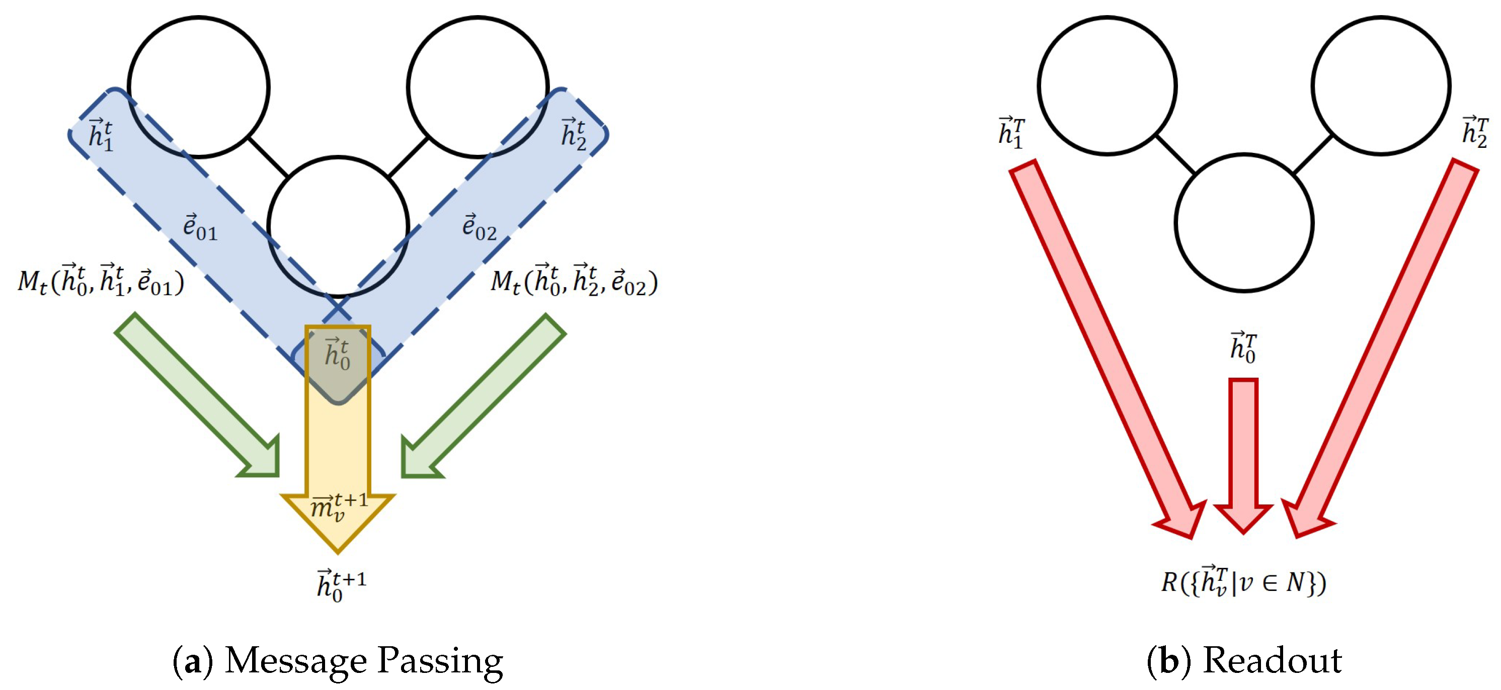
Figure 1.
The message-passing neural network (MPNN) framework. (a) One message passing step for Node 0. The blue section indicates the process of the calculation of individual messages; the green arrows indicate the aggregation; the yellow arrow represents the node feature update. (b) The readout phase.
Figure 2.
Overview of different systems, models, and tasks discussed in this work for graph neural network methodologies in materials research.
Figure 2.
Overview of different systems, models, and tasks discussed in this work for graph neural network methodologies in materials research.
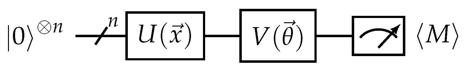
Figure 3.
Quantum variational model circuit. U is a quantum encoding circuit that maps the input data into a quantum state, while V is the quantum neural network (QNN) that can be trained. The model output is the expectation value of an observable M.
Figure 3.
Quantum variational model circuit. U is a quantum encoding circuit that maps the input data into a quantum state, while V is the quantum neural network (QNN) that can be trained. The model output is the expectation value of an observable M.
Figure 4.
An example of quantum encoding. Individual elements of an input classical vector are used as the rotation angles of rotation Pauli X (RX) gates, creating a quantum state.
Figure 4.
An example of quantum encoding. Individual elements of an input classical vector are used as the rotation angles of rotation Pauli X (RX) gates, creating a quantum state.
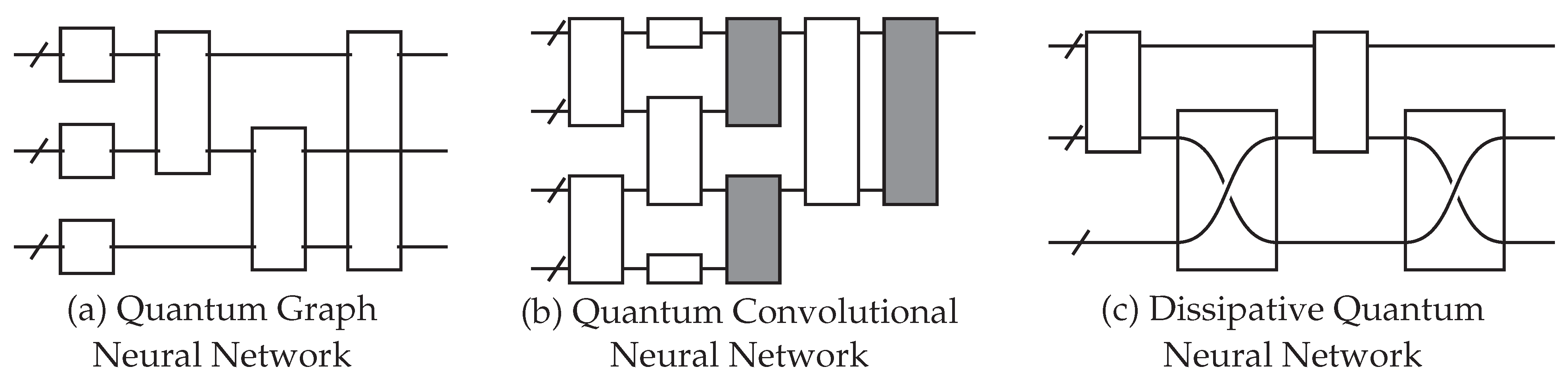
Figure 5.
Examples of different QNN architecture designs. Each empty gate has trainable parameters. (a) The quantum graph neural network (QGNN) is used for processing graph-structured data. The circuit structure is dependent on the input graph. (b) The quantum convolutional neural network has a convolution operator (white) and a pooling operator (gray). (c) The dissipative quantum neural network represents each neuron as a group of qubits, and unitary operators transform one layer to another. This example is an input layer of one perceptron (the top group of qubits) being mapped to a layer of two perceptrons (the bottom two groups of qubits).
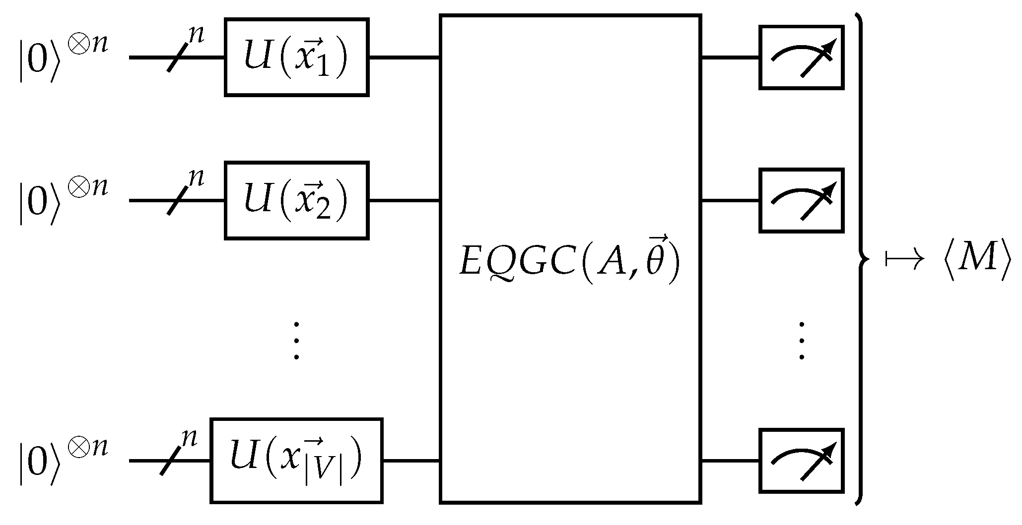
Figure 6.
The equivariant quantum graph circuit (EQGC) framework. Given an input graph with nodes V, adjacency matrix A, and node features , the circuit drawn above is used. The EQGC is equivariant on the permutation of nodes and is trainable, while the measurement is invariant on the permutation of nodes.
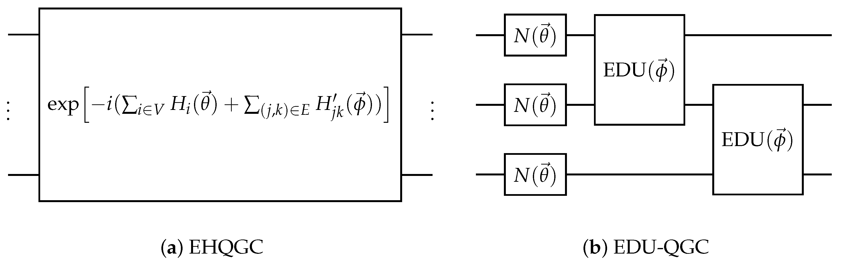
Figure 7.
Examples of two different EQGC implementation methods. (a) is an example of the equivariant Hamiltonian quantum graph circuit (EHQGC), and (b) is an example of the equivariantly diagonalizable unitary quantum graph circuit (EDU-QGC).
Figure 7.
Examples of two different EQGC implementation methods. (a) is an example of the equivariant Hamiltonian quantum graph circuit (EHQGC), and (b) is an example of the equivariantly diagonalizable unitary quantum graph circuit (EDU-QGC).
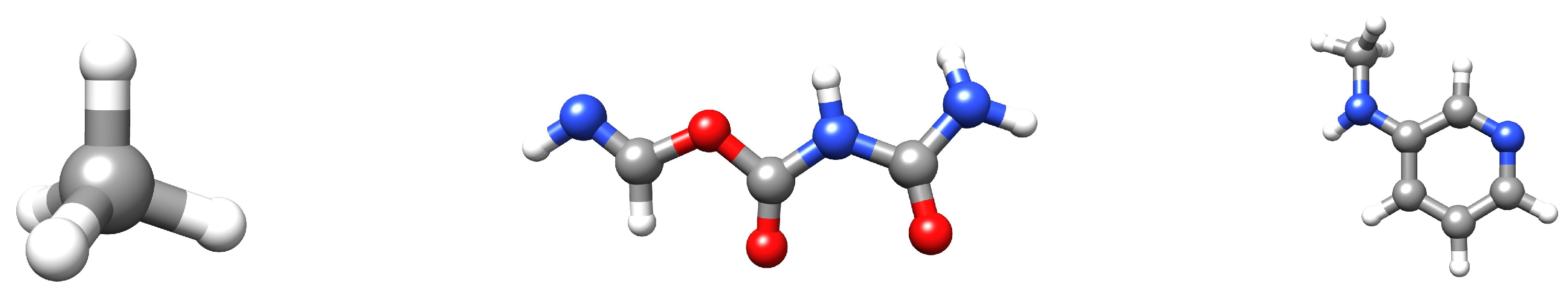
Figure 8.
Examples of molecules in the QM9 dataset. The white atoms are hydrogen; the grey atoms are carbon; the red atoms are oxygen; the blue atoms are nitrogen. Visualization was achieved with UCSF Chimera [
83].
Figure 8.
Examples of molecules in the QM9 dataset. The white atoms are hydrogen; the grey atoms are carbon; the red atoms are oxygen; the blue atoms are nitrogen. Visualization was achieved with UCSF Chimera [
83].
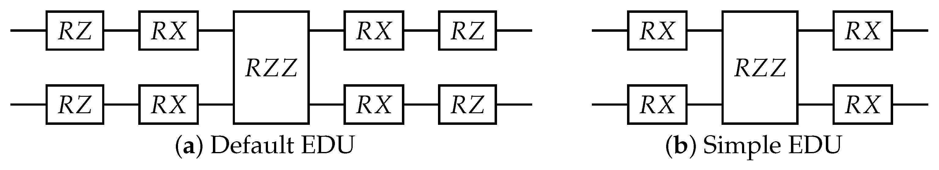
Figure 9.
The equivariantly diagonalizable unitary (EDU) circuit design. The single qubit gates are parameterized with trainable link variables, while the diagonal two-qubit gate is parameterized with a trainable parameter dependent on the layer. (a) The default EDU was used throughout the experiment. If not otherwise specified, this is the EDU that was used. (b) A simpler EDU was used to test the effect of the expressibility of the EDU on the model performance.
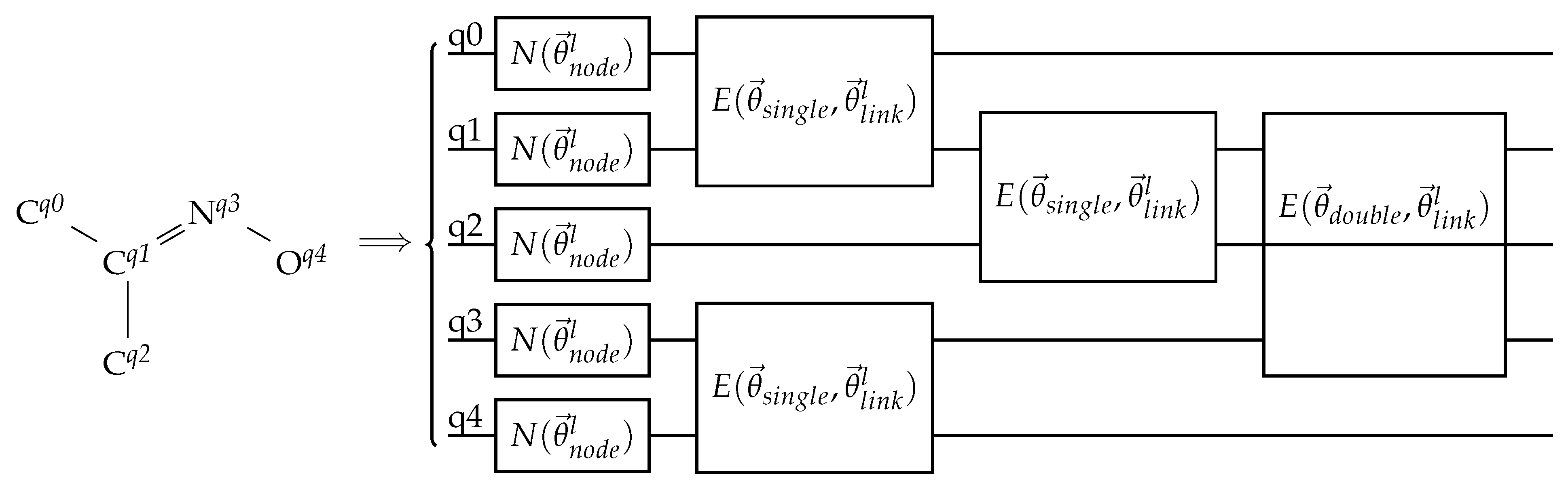
Figure 10.
An example of a bond-information-encoding EDU-QGC layer. The input molecule is drawn on the left without its hydrogen atoms. The superscripts are the assigned qubit indices. The circuit on the right shows one EDU-QGC layer. N and E are node-local unitaries and EDUs, respectively. and are trainable parameters that depend on the layer number l, while and are trainable variables that depend on the bond order. Note that the single bonds are applied first, then the double bond.
Figure 11.
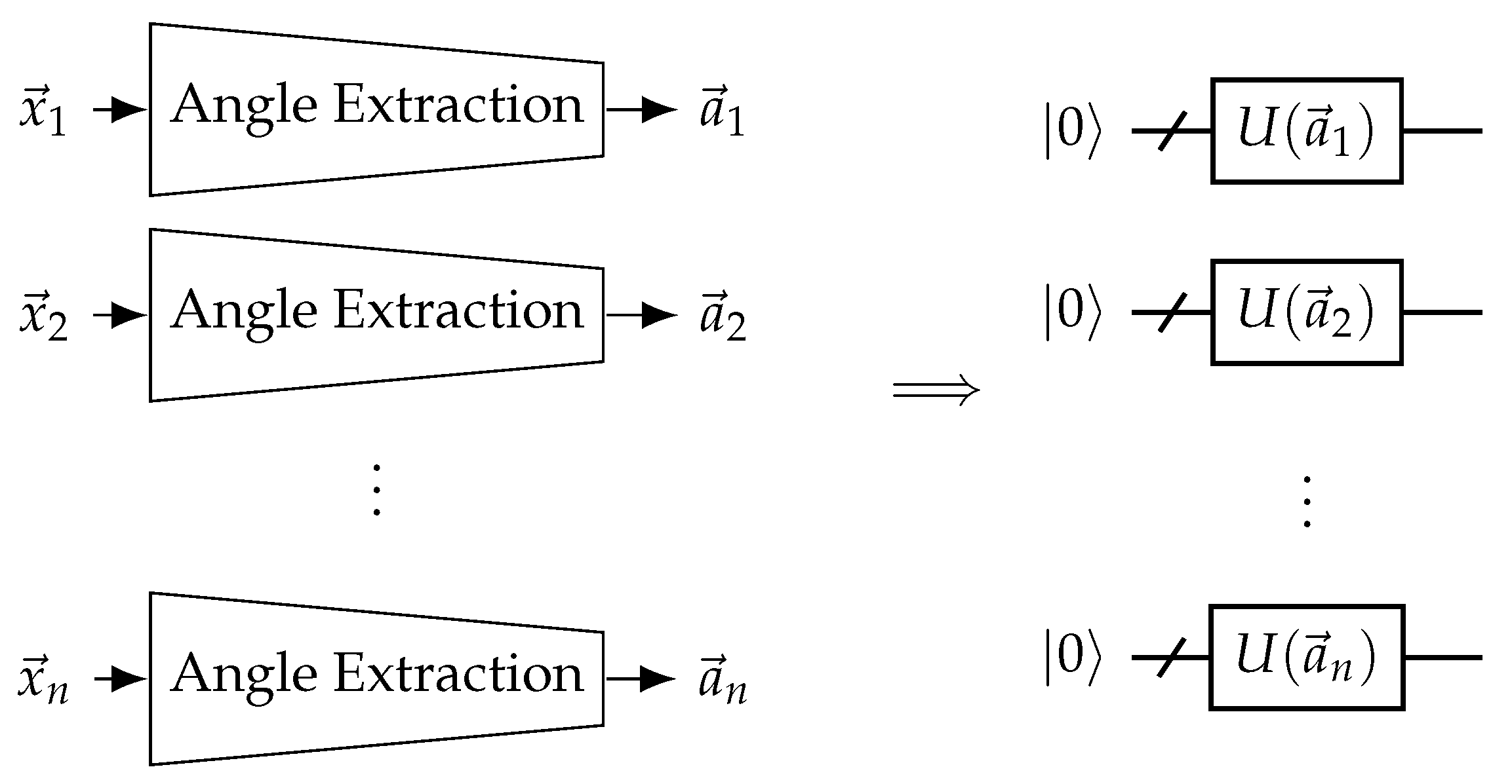
Neural network-assisted quantum encoding EQGCs. Explicit input features are transformed into rotation angles for the QGNN to use for encoding using a trainable angle extraction neural network. In the case of EQGCs, the same angle extraction network should be used for all nodes.
Figure 11.
Neural network-assisted quantum encoding EQGCs. Explicit input features are transformed into rotation angles for the QGNN to use for encoding using a trainable angle extraction neural network. In the case of EQGCs, the same angle extraction network should be used for all nodes.
Figure 12.
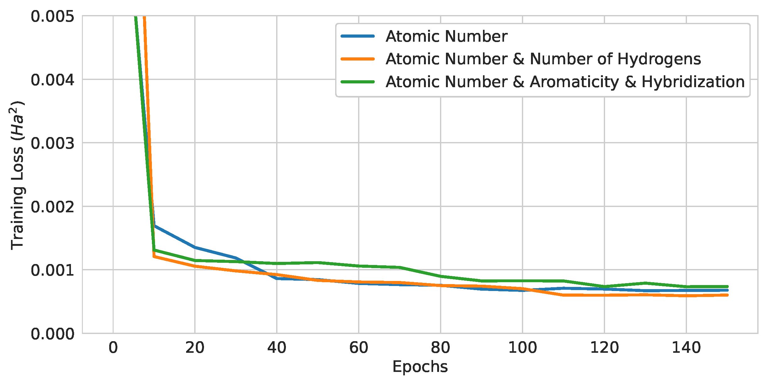
Training curves of 3-layer pure QGNNs with different encoding strategies.
Figure 12.
Training curves of 3-layer pure QGNNs with different encoding strategies.
Figure 13.
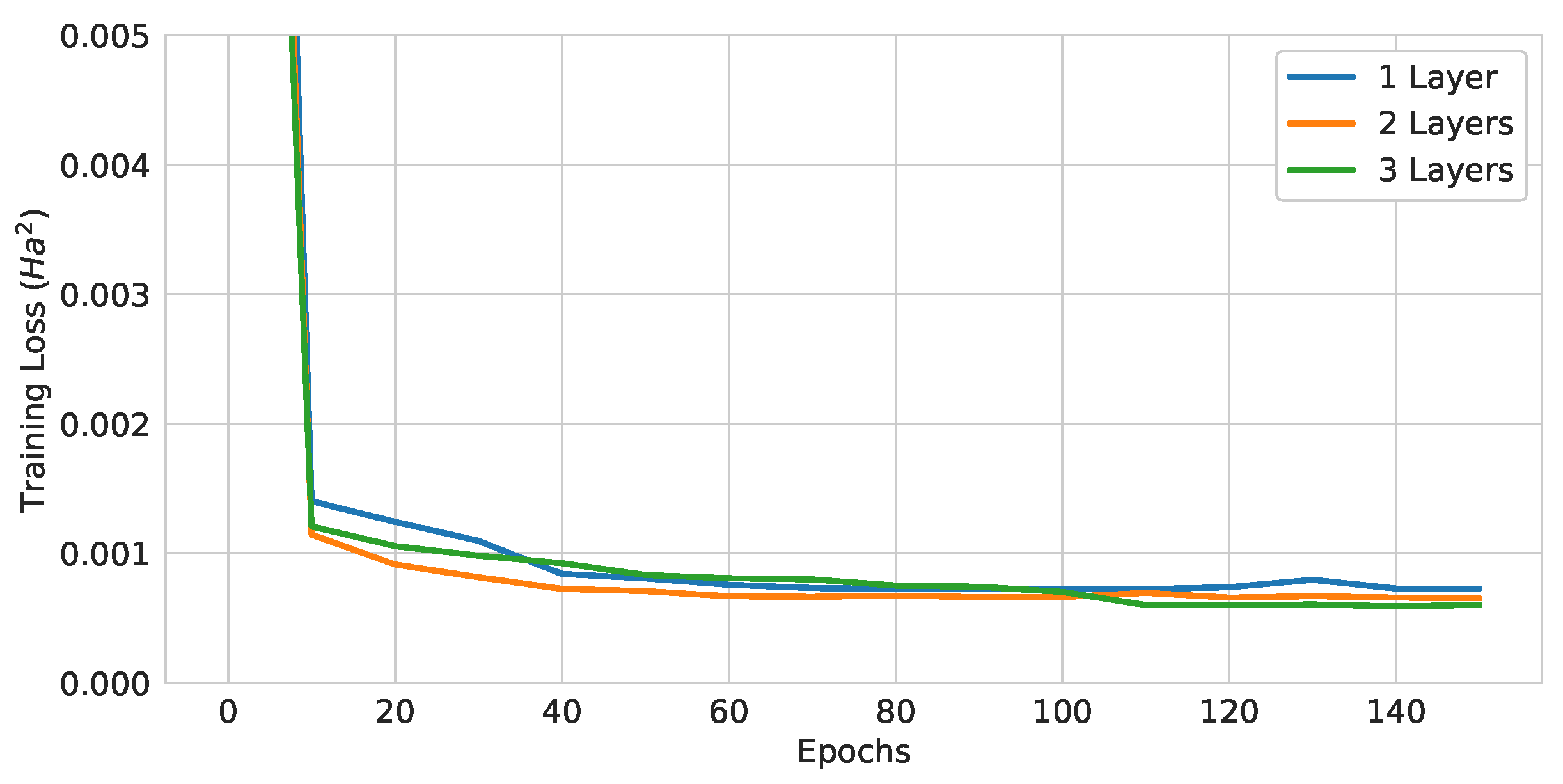
Training curves of pure QGNNs with different numbers of layers.
Figure 13.
Training curves of pure QGNNs with different numbers of layers.
Figure 14.
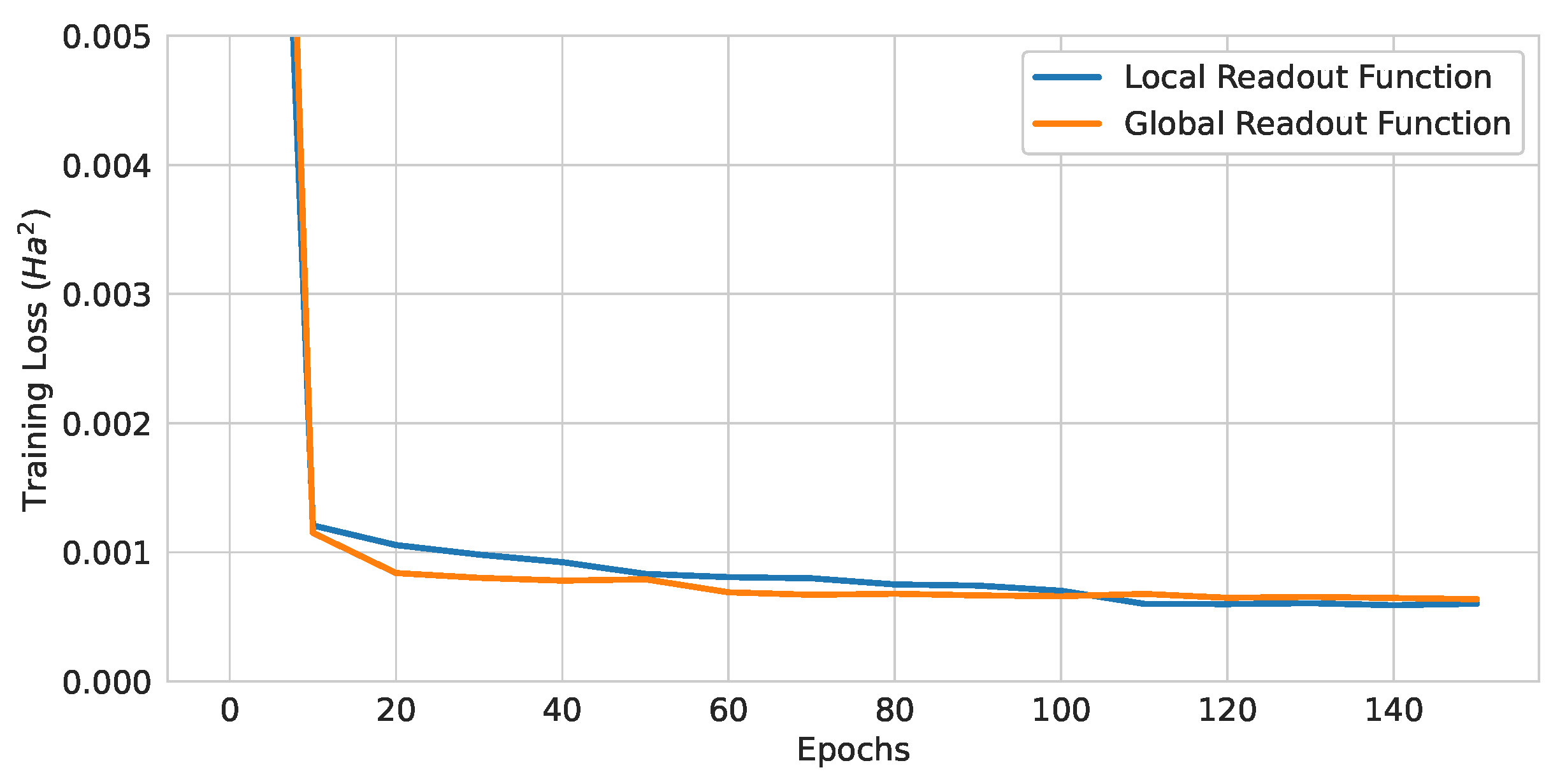
Training curves of QGNNs with different readout functions.
Figure 14.
Training curves of QGNNs with different readout functions.
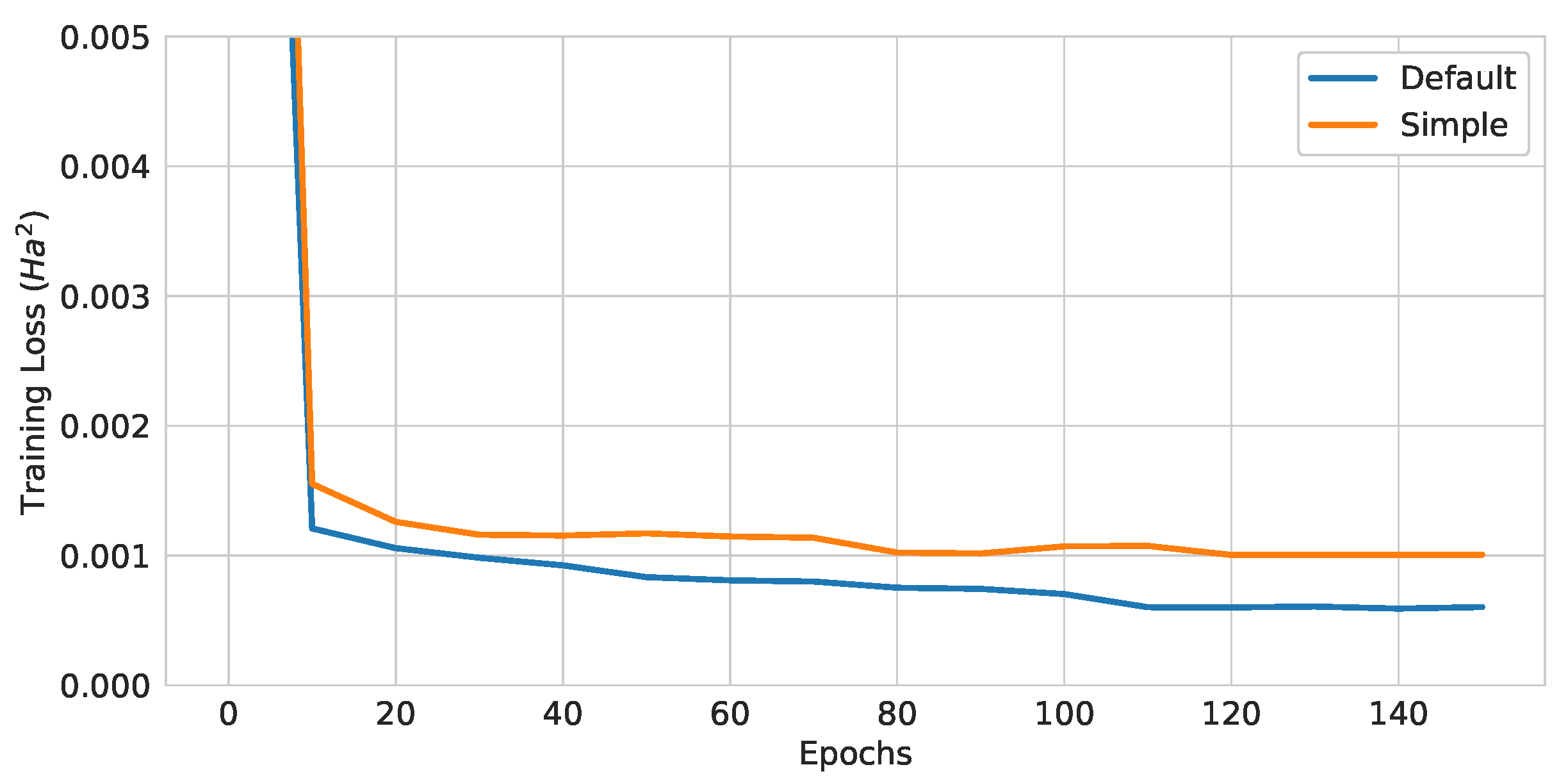
Figure 15.
Training curves of QGNNs with different EDU-QGC architectures.
Figure 15.
Training curves of QGNNs with different EDU-QGC architectures.
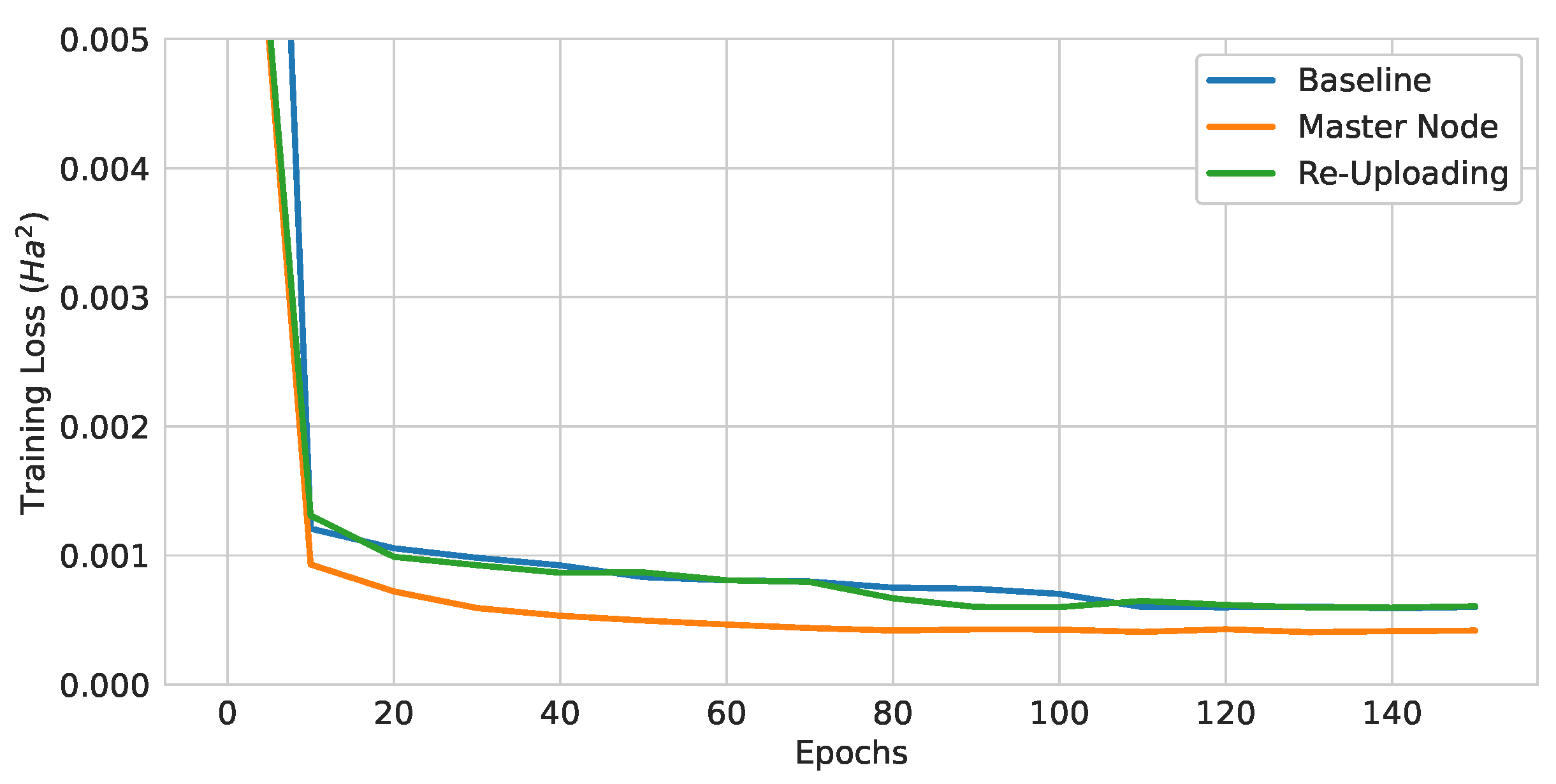
Figure 16.
Training curves of QGNNs with different modifications for higher expressibility.
Figure 16.
Training curves of QGNNs with different modifications for higher expressibility.
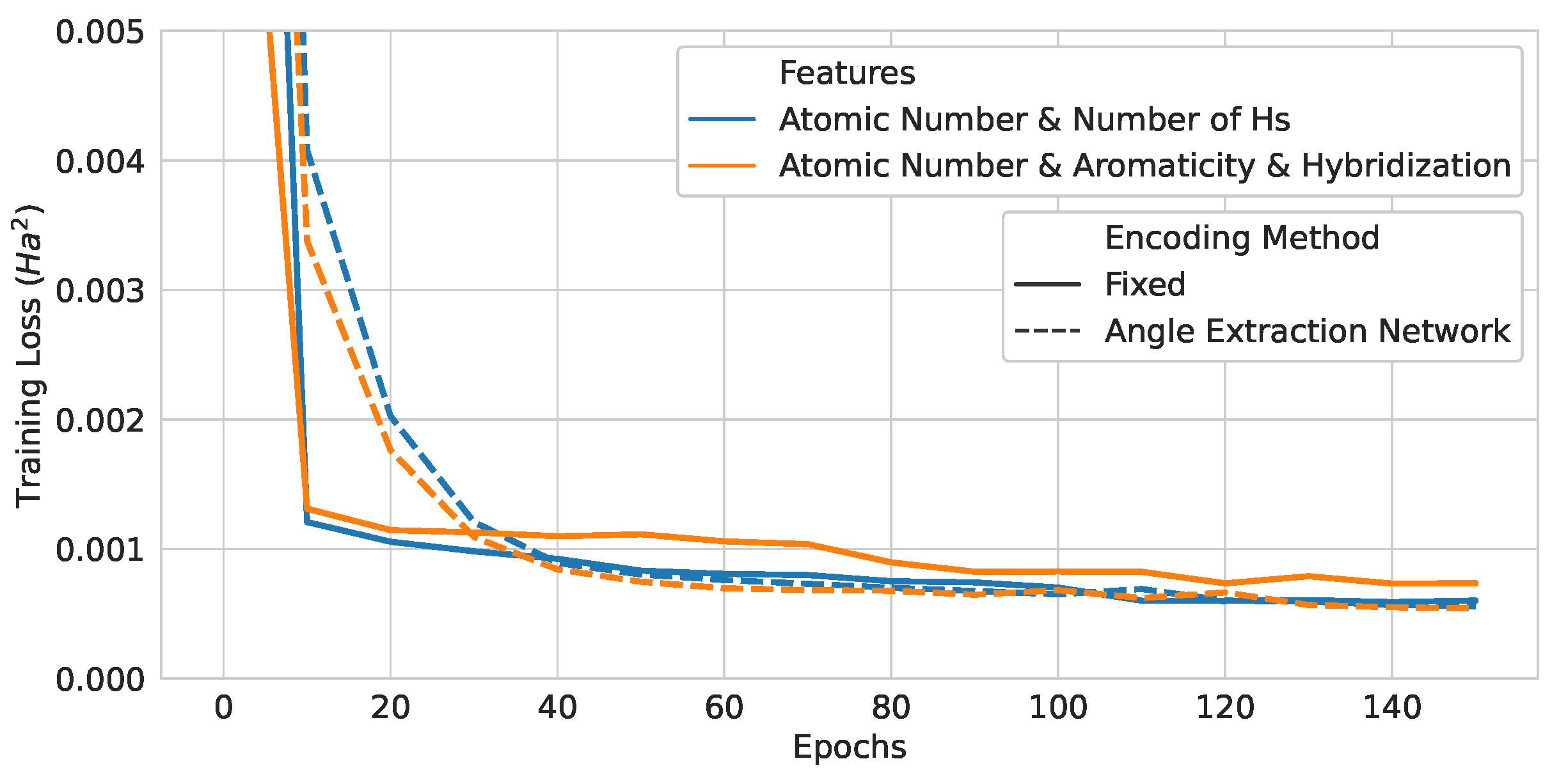
Figure 17.
Training curves of neural-network-assisted quantum encoding models and their quantum counterparts.
Figure 17.
Training curves of neural-network-assisted quantum encoding models and their quantum counterparts.
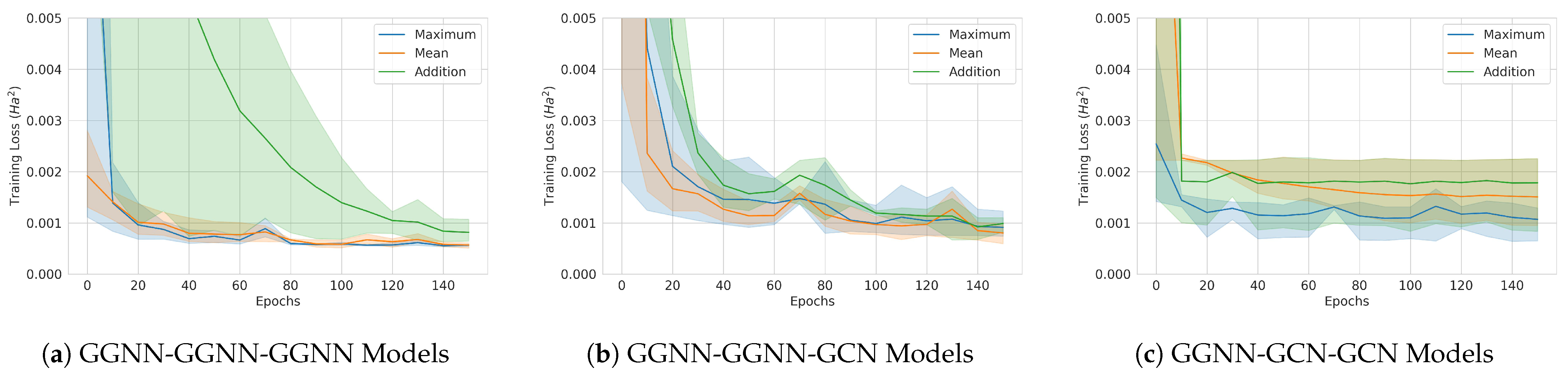
Figure 18.
Classical model training curves. The solid lines are averages over 3 runs, and the 95% confidence intervals are also shown. (a) GGNN-GGNN-GGNN model. (b) GGNN-GGNN-GCN model. (c) GGNN-GCN-GCN model.
Figure 18.
Classical model training curves. The solid lines are averages over 3 runs, and the 95% confidence intervals are also shown. (a) GGNN-GGNN-GGNN model. (b) GGNN-GGNN-GCN model. (c) GGNN-GCN-GCN model.
Figure 19.
Absolute prediction error distribution of quantum, hybrid, and classical models on the test dataset molecules. The molecules for which the models have accurate and inaccurate predictions are drawn.
Figure 19.
Absolute prediction error distribution of quantum, hybrid, and classical models on the test dataset molecules. The molecules for which the models have accurate and inaccurate predictions are drawn.
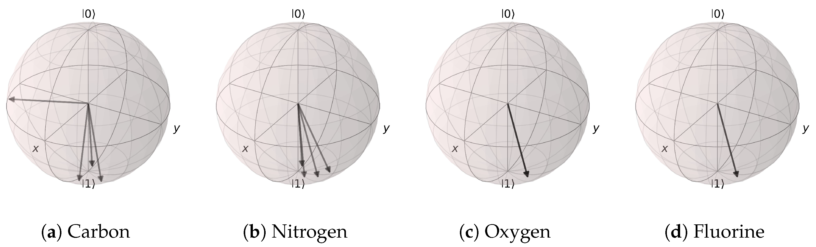
Figure 20.
Angle extraction network results for the (Atomic Number, Aromaticity, and Hybridization) model. All possible atomic features are grouped together by the atom type. (a) Carbon atom states are mostly distributed near |1〉, except for the non-aromatic hybridization case. (b) Nitrogen, (c) oxygen, and (d) fluorine atoms are all distributed near the |1〉 state.
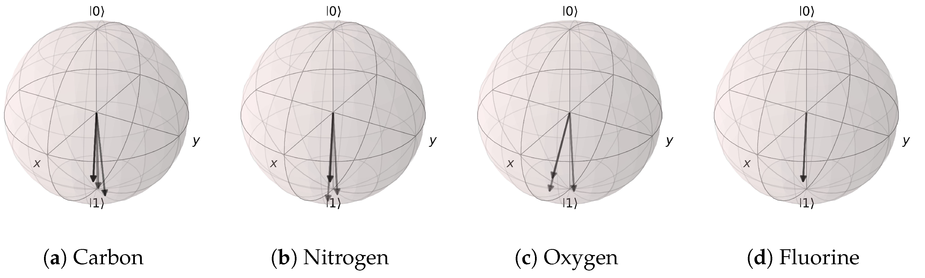
Figure 21.
Angle extraction network results for the (Atomic Number and Number of Hydrogens) model. The states are distributed near |1〉. (a) carbon atoms, (b) nitrogen atoms, (c) oxygen atoms, and (d) fluorine atoms.
Figure 21.
Angle extraction network results for the (Atomic Number and Number of Hydrogens) model. The states are distributed near |1〉. (a) carbon atoms, (b) nitrogen atoms, (c) oxygen atoms, and (d) fluorine atoms.
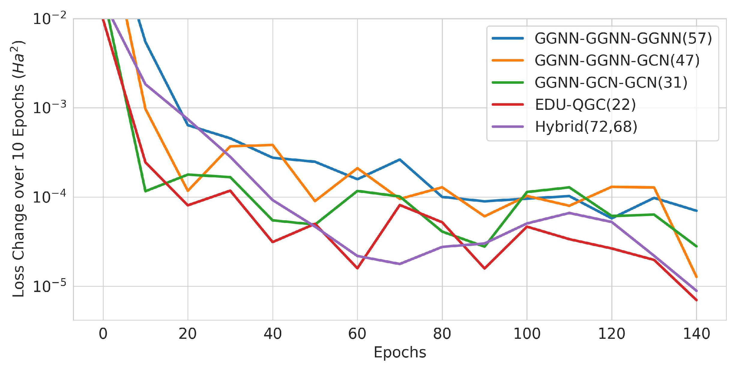
Figure 22.
Change in training loss in 10-epoch intervals. The solid lines are averages of the runs, and the x axis is the beginning epoch number of the interval. The number of trainable variables is written in the legend in parenthesis.
Figure 22.
Change in training loss in 10-epoch intervals. The solid lines are averages of the runs, and the x axis is the beginning epoch number of the interval. The number of trainable variables is written in the legend in parenthesis.
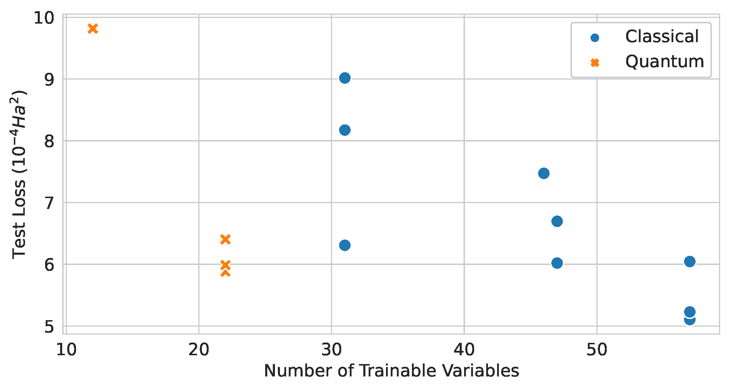
Figure 23.
Relationship between the number of trainable variables and the test loss values of classical and quantum graph network models.
Figure 23.
Relationship between the number of trainable variables and the test loss values of classical and quantum graph network models.
Table 1.
Node features and link features in the processed QM9 dataset.
Table 1.
Node features and link features in the processed QM9 dataset.
| | Feature | Explanation → Data Type |
|---|
Nodes
→ Non-Hydrogen Atoms | Atomic Number | C/N/O/F → Integer |
| Number of Bonded Hs | 0~4 → Integer |
| Aromaticity | True/False → Boolean |
| Hybridization | Integer |
Links
→ Bonds | Bond Type | Single/Aromatic/Double/Triple
→ Integer |
Table 2.
Quantum encoding methods. z is the atomic number; is the number of bonded hydrogen atoms; a is the aromaticity as True(1)/False(0); h is the hybridization type (: 1, : 2, : 3).
Table 2.
Quantum encoding methods. z is the atomic number; is the number of bonded hydrogen atoms; a is the aromaticity as True(1)/False(0); h is the hybridization type (: 1, : 2, : 3).
| | Atomic Number | Atomic Number and Number of Hydrogens | Atomic Number, Aromaticity, and Hybridization |
|---|
| RY Rotation Angle |
| | |
| RZ Rotation Angle |
| | |
Table 3.
Test loss values of pure QGNNs with different encoding.
Table 3.
Test loss values of pure QGNNs with different encoding.
| Encoding Method | Test MSE
| Test RMSE
| Test MAE
|
|---|
| Atomic Number | 6.3394 | 2.5178 | 1.9975 |
| Atomic Number and Number of Hydrogens | 5.8806 | 2.4250 | 1.8793 |
| Atomic Number, Aromaticity, and Hybridization | 7.1288 | 2.6700 | 2.0811 |
Table 4.
Test loss values of pure QGNNs with different numbers of layers.
Table 4.
Test loss values of pure QGNNs with different numbers of layers.
| Number of Layers | Test MSE
| Test RMSE
| Test MAE
|
|---|
| 1 | 7.3759 | 2.7159 | 2.1400 |
| 2 | 6.5147 | 2.5524 | 2.0174 |
| 3 | 5.8806 | 2.4250 | 1.8793 |
Table 5.
Test loss values of pure QGNNs with different readout functions.
Table 5.
Test loss values of pure QGNNs with different readout functions.
| Readout Function | Test MSE
| Test RMSE
| Test MAE
|
|---|
| Local | 5.8806 | 2.4250 | 1.8793 |
| Global | 6.4033 | 2.5305 | 1.9307 |
Table 6.
Test loss values of pure QGNNs with different EDU-QGC architectures.
Table 6.
Test loss values of pure QGNNs with different EDU-QGC architectures.
| Model | Test MSE
| Test RMSE
| Test MAE
|
|---|
| Default | 5.8806 | 2.4250 | 1.8793 |
| Simple | 9.8162 | 3.1331 | 2.5045 |
Table 7.
Test loss values of pure QGNNs with different modifications to the baseline model.
Table 7.
Test loss values of pure QGNNs with different modifications to the baseline model.
| Model | Test MSE
| Test RMSE
| Test MAE
|
|---|
| Baseline | 5.8806 | 2.4250 | 1.8793 |
| Baseline and Master Node | 4.0372 | 2.0093 | 1.5106 |
| Baseline and Re-Uploading | 5.9863 | 2.4467 | 1.9379 |
Table 8.
Test loss values of neural-network-assisted quantum encoding models and their quantum counterparts.
Table 8.
Test loss values of neural-network-assisted quantum encoding models and their quantum counterparts.
| Node Features | Encoding Method | Test MSE
| Test RMSE
| Test MAE
|
|---|
| Atomic Number | Fixed | 5.8806 | 2.4250 | 1.8793 |
| and Number of Hydrogens | Angle Extraction Network | 5.3127 | 2.3049 | 1.7846 |
| Atomic Number, | Fixed | 7.1288 | 2.6700 | 2.0811 |
| Aromaticity, and Hybridization | Angle Extraction Network | 5.4597 | 2.3366 | 1.8097 |
Table 9.
Test loss values of classical graph neural network models.
Table 9.
Test loss values of classical graph neural network models.
| Architecture | GGNN Aggregation | Test MSE
() | Test RMSE
| Test MAE
|
|---|
| | Addition | 6.0449 | 2.4586 | 1.9597 |
| GGNN-GGNN-GGNN | Mean | 5.1052 | 2.2595 | 1.7742 |
| | Max | 5.2289 | 2.2867 | 1.8053 |
| | Addition | 6.6965 | 2.5878 | 2.0311 |
| GGNN-GGNN-GCN | Mean | 6.0202 | 2.4536 | 1.9460 |
| | Max | 7.4732 | 2.7337 | 2.1468 |
| | Addition | 8.1737 | 2.8590 | 2.2079 |
| GGNN-GCN-GCN | Mean | 9.0177 | 3.0029 | 2.4088 |
| | Max | 6.3081 | 2.5116 | 2.0143 |
Table 10.
Mean absolute error values of quantum, hybrid, and classical models on molecules with and without aromatic rings.
Table 10.
Mean absolute error values of quantum, hybrid, and classical models on molecules with and without aromatic rings.
| Model | With Aromatic Rings
| Without Aromatic Rings
|
|---|
| Quantum (Master Node) | 1.9277 | 1.4128 |
| Quantum (Baseline) | 2.2509 | 1.7921 |
| Hybrid | 1.9323 | 1.7499 |
| Classical | 1.9820 | 1.7254 |


