
Damage Evolution of Hot Stamped Boron Steels Subjected to Various Stress States: Macro/Micro-Scale Experiments and Simulations

Abstract
1. Introduction
2. Materials and Methods
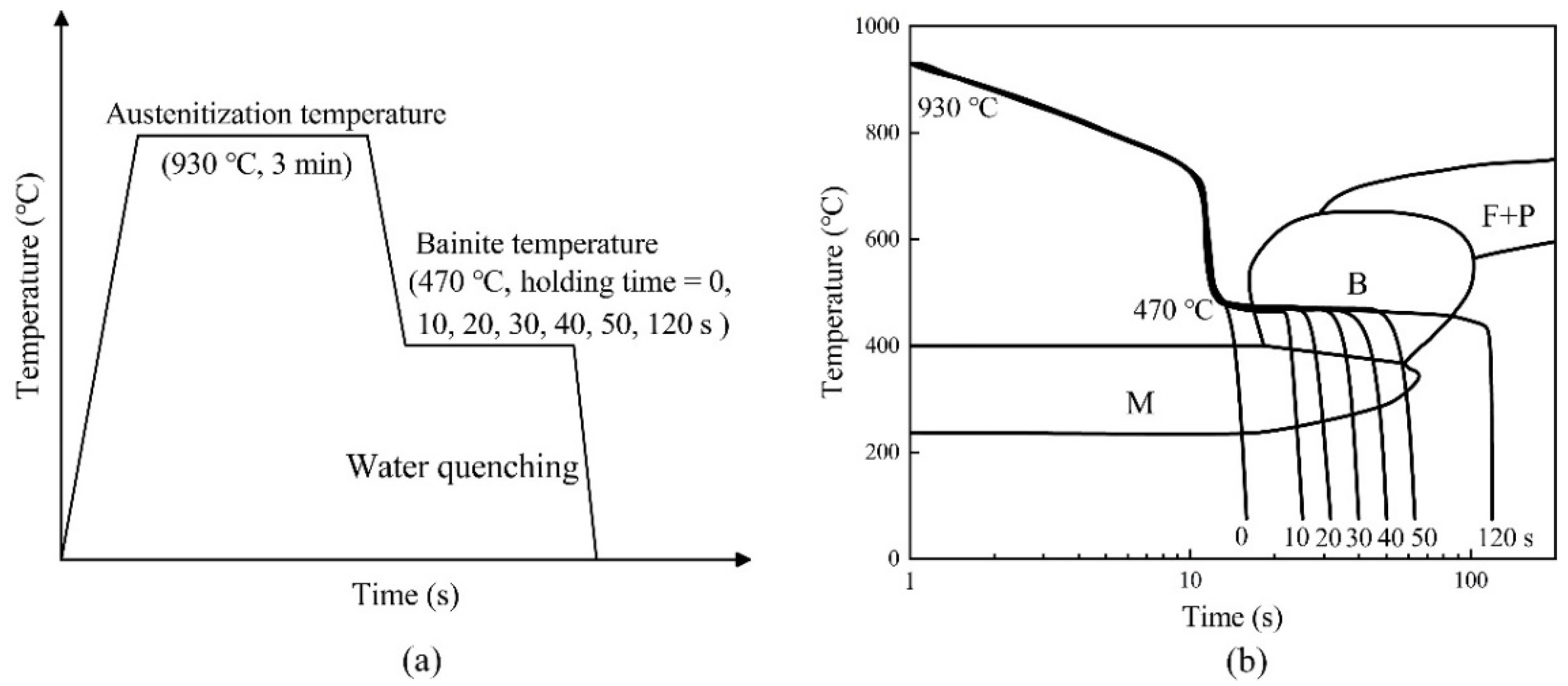
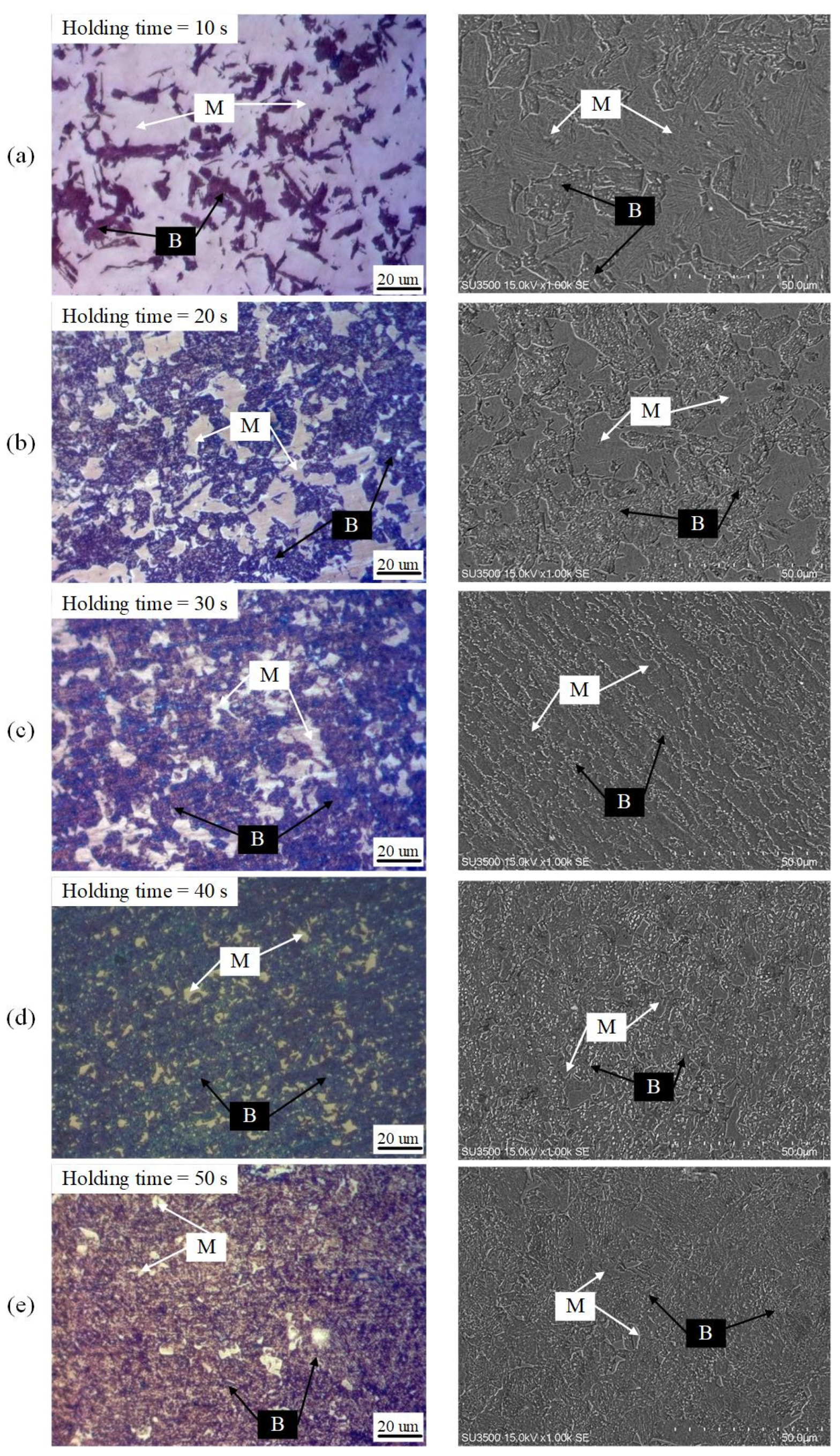
2.1. Material Characterization
2.2. Tensile Tests
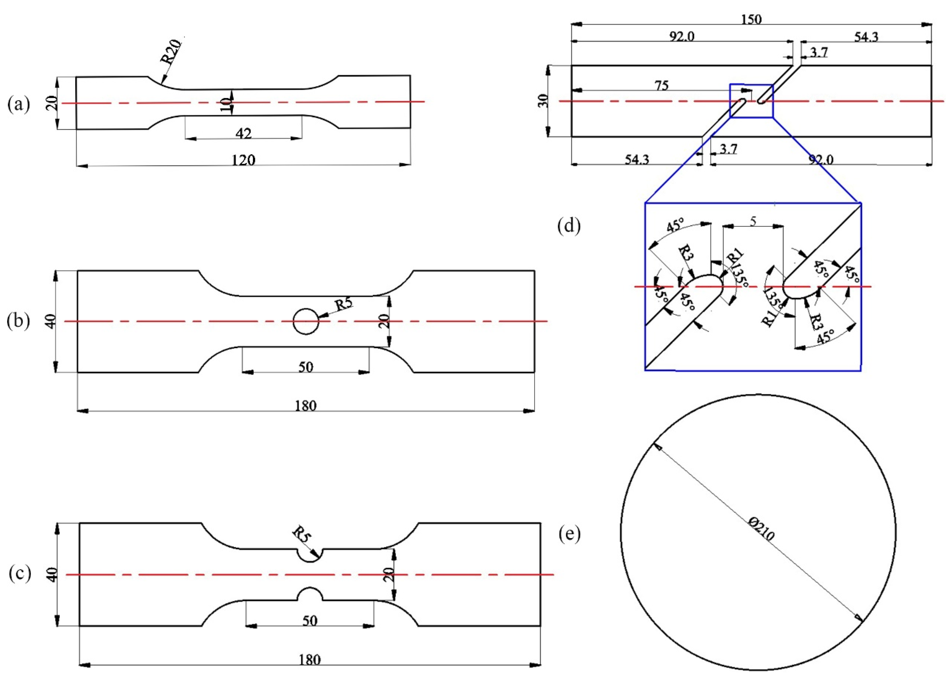
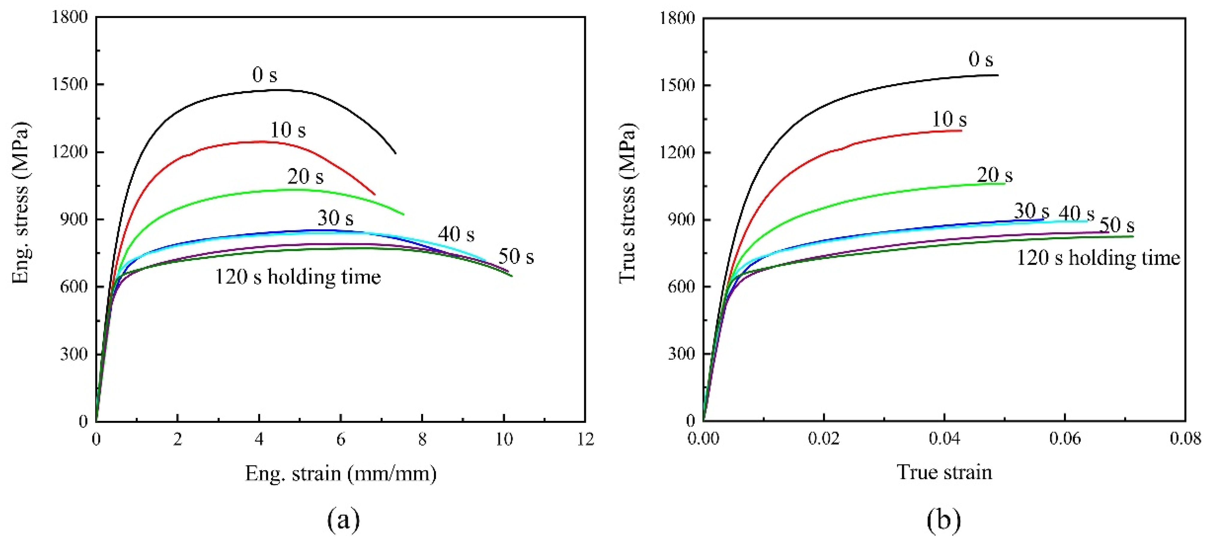
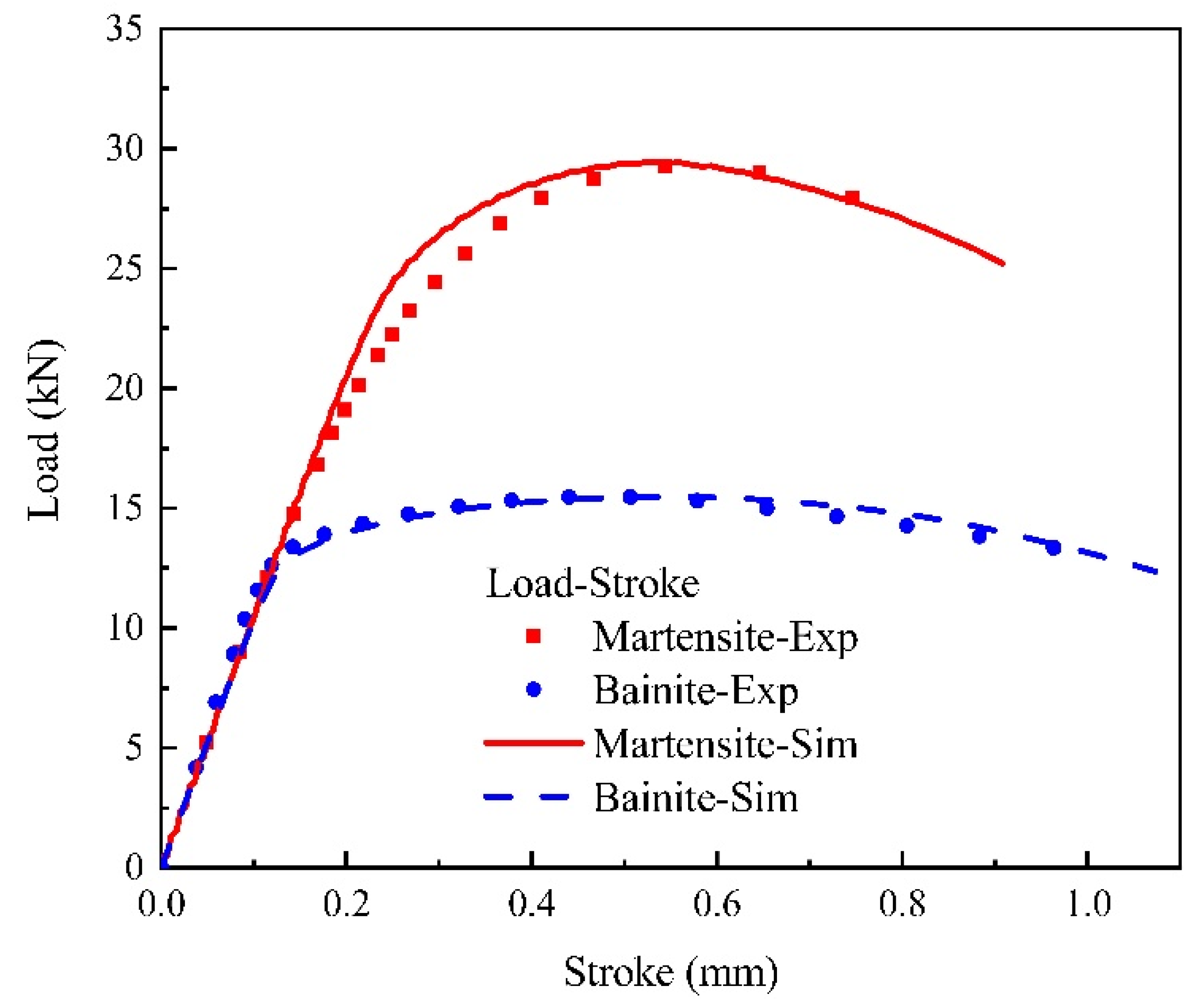
2.2.1. Dogbone Tensile Test
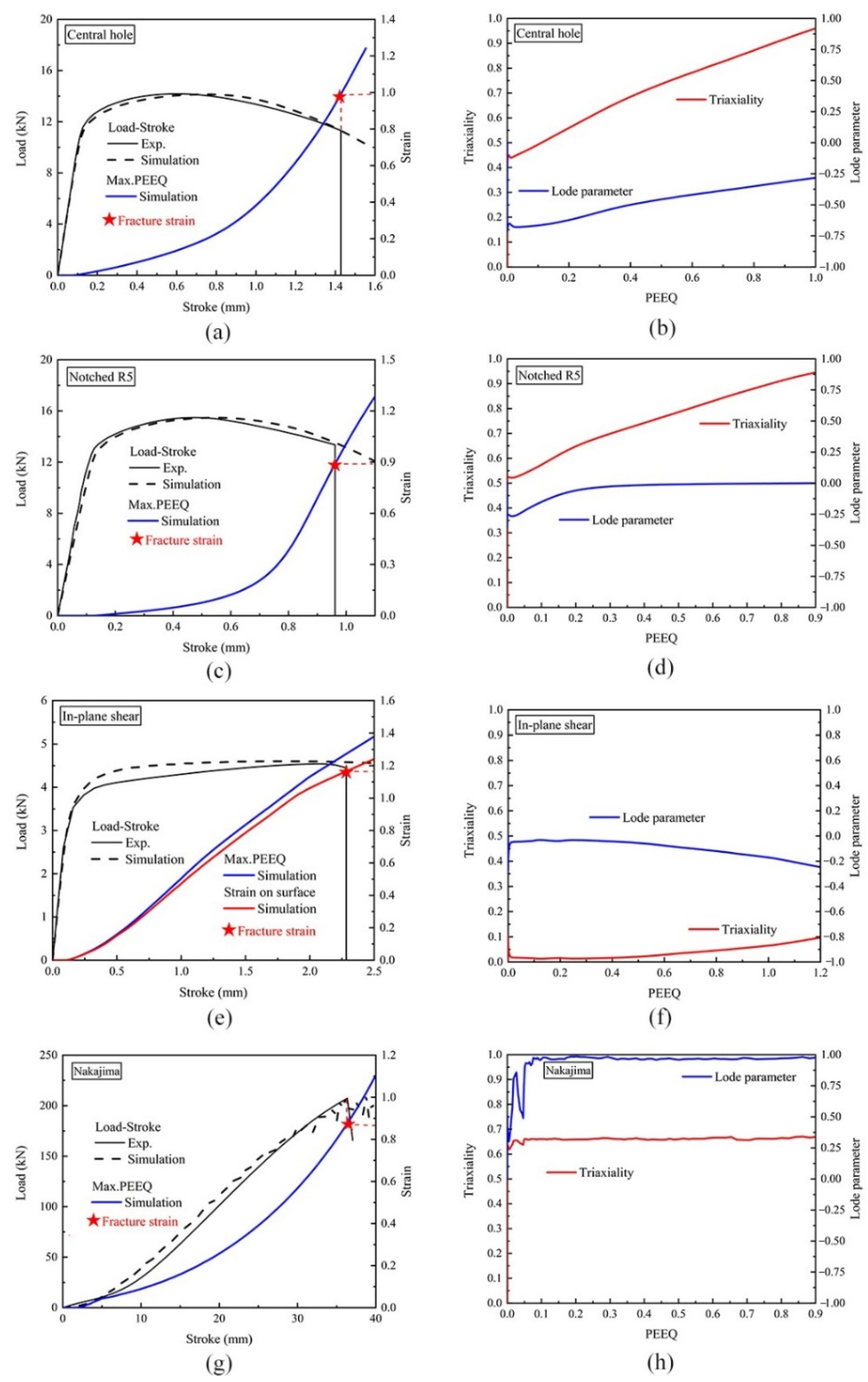
2.2.2. Tensile Tests in Different Stress States
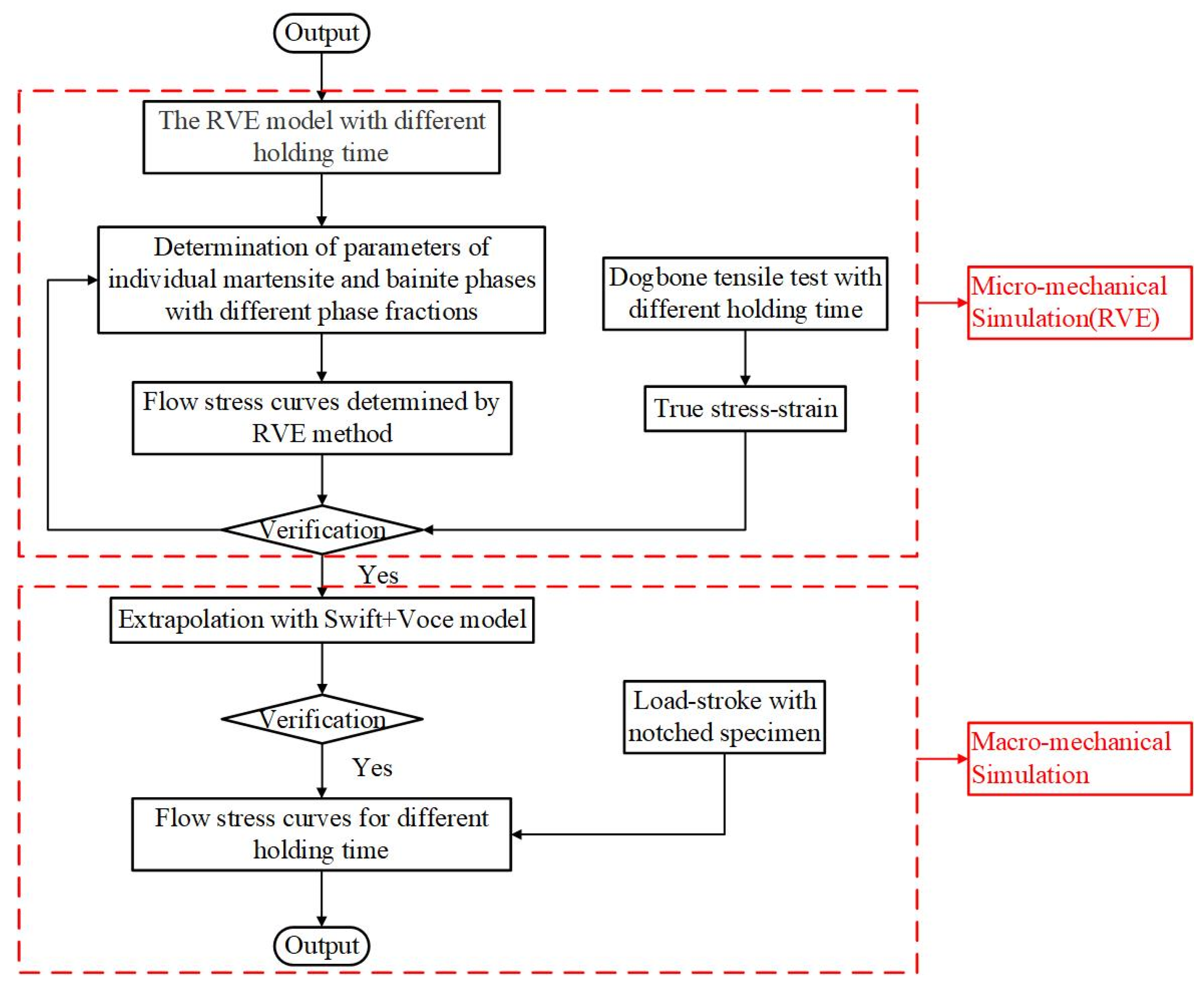
3. Micro-Mechanical Modeling
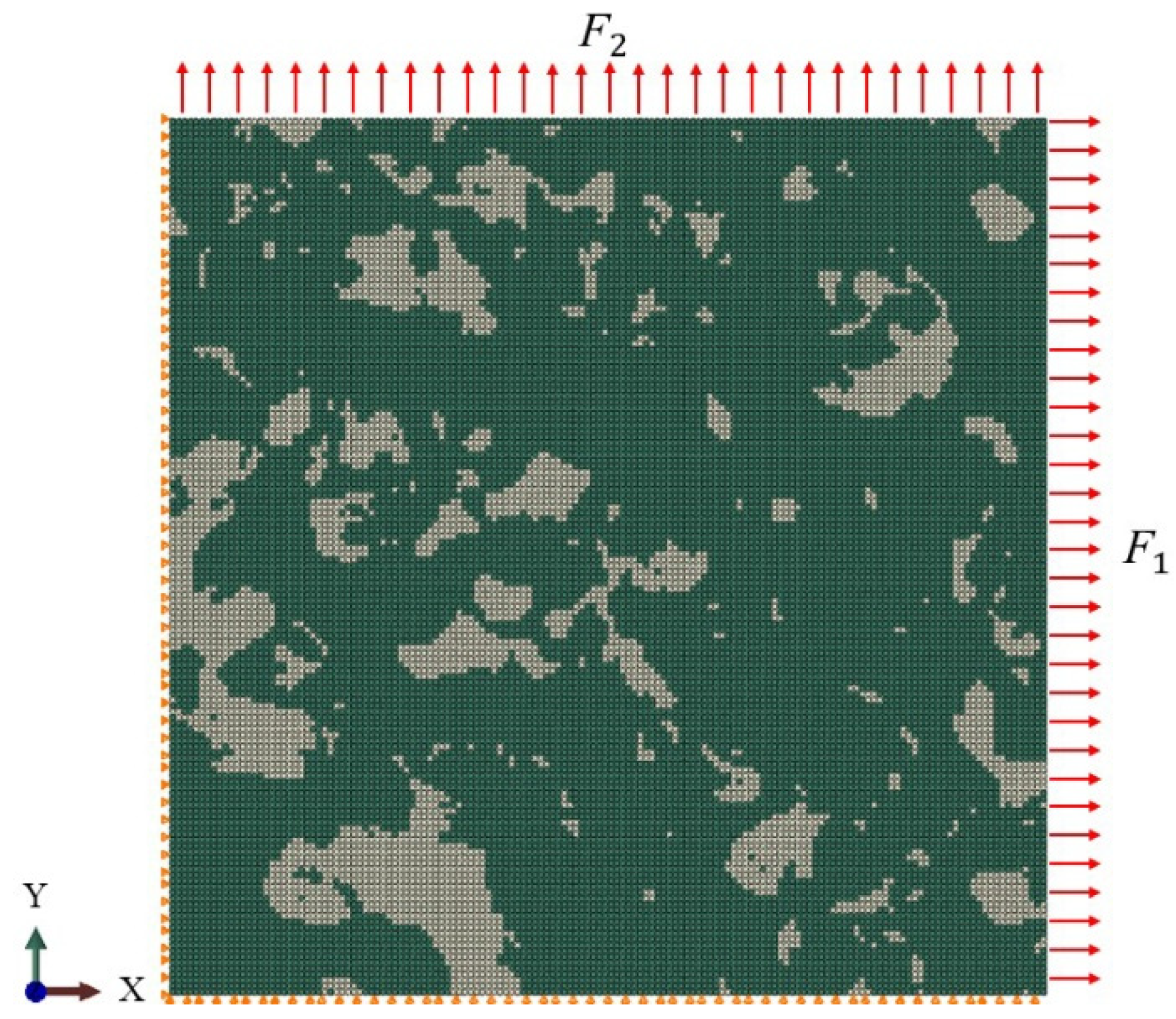
3.1. Representative Volume Element (RVE) Approach
3.2. Constitutive Modeling
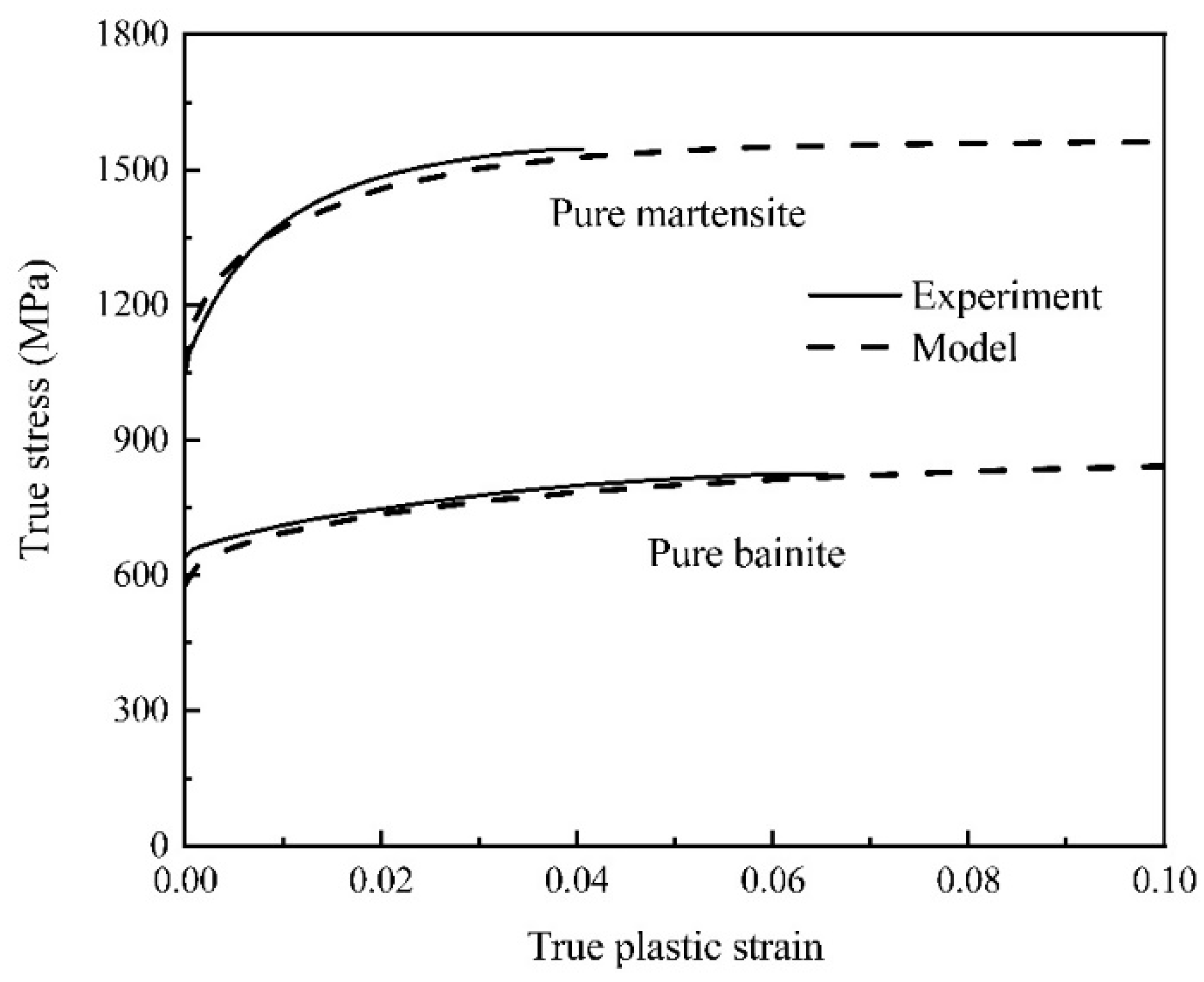
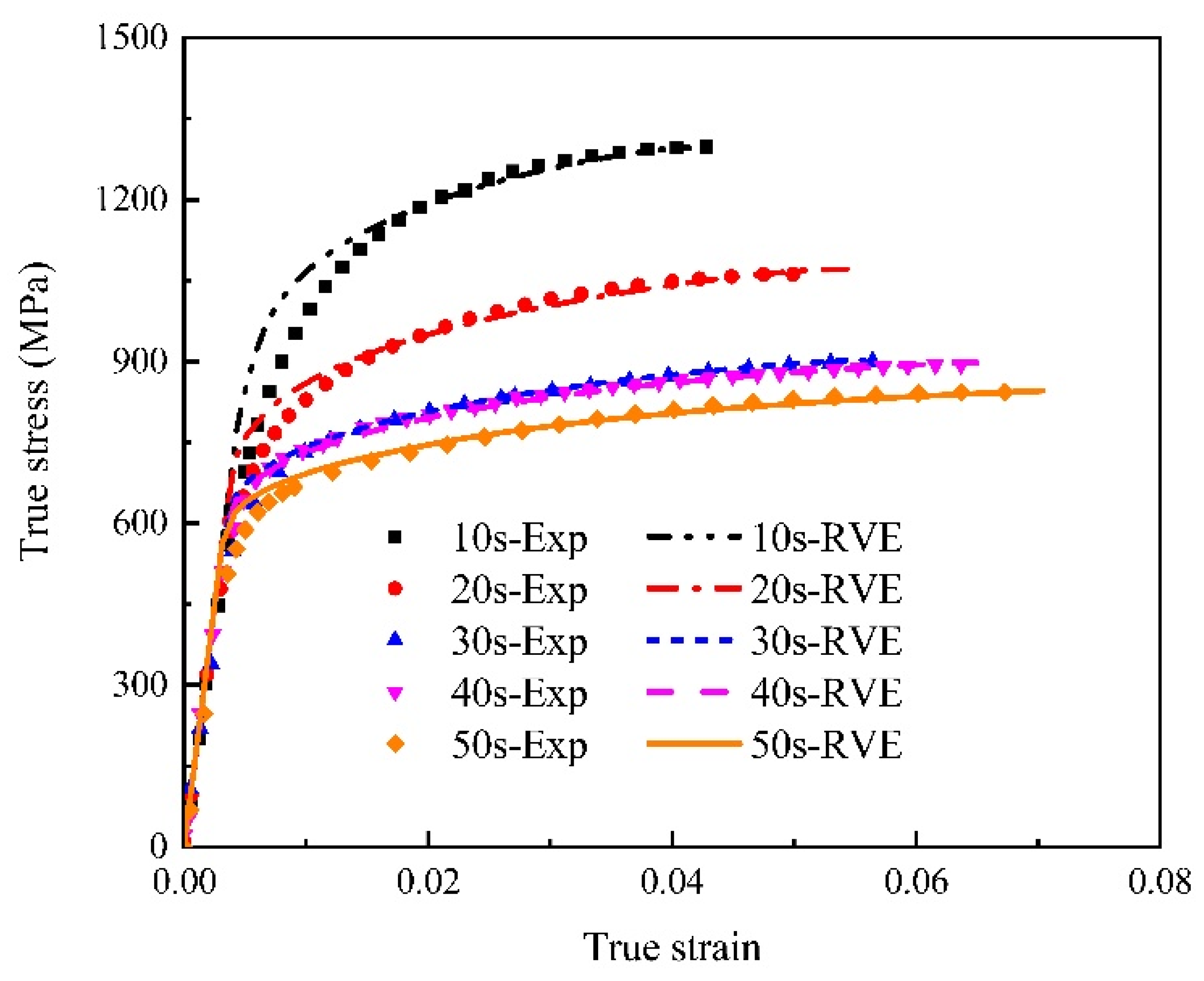
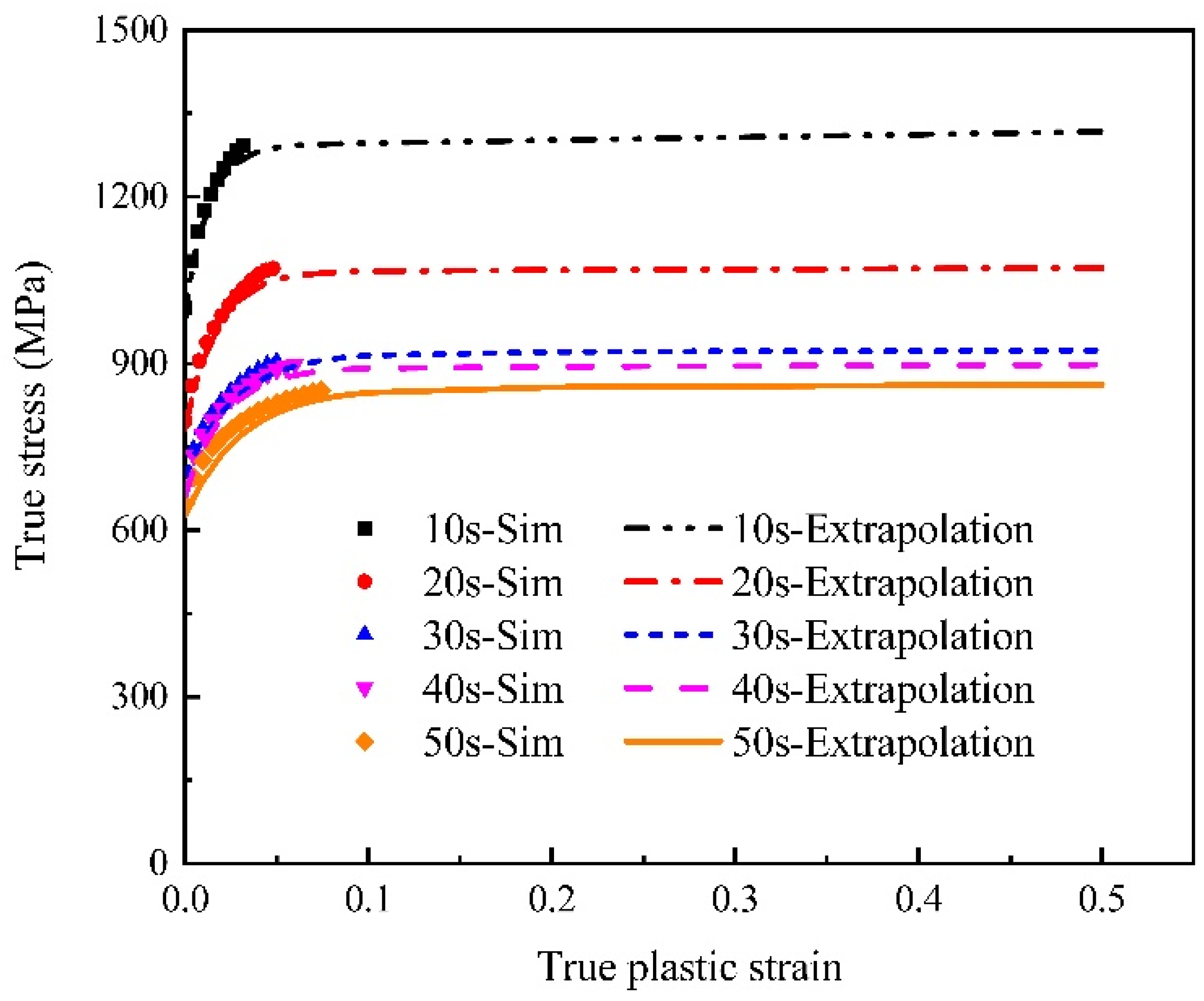
3.2.1. Stress–Strain Curve
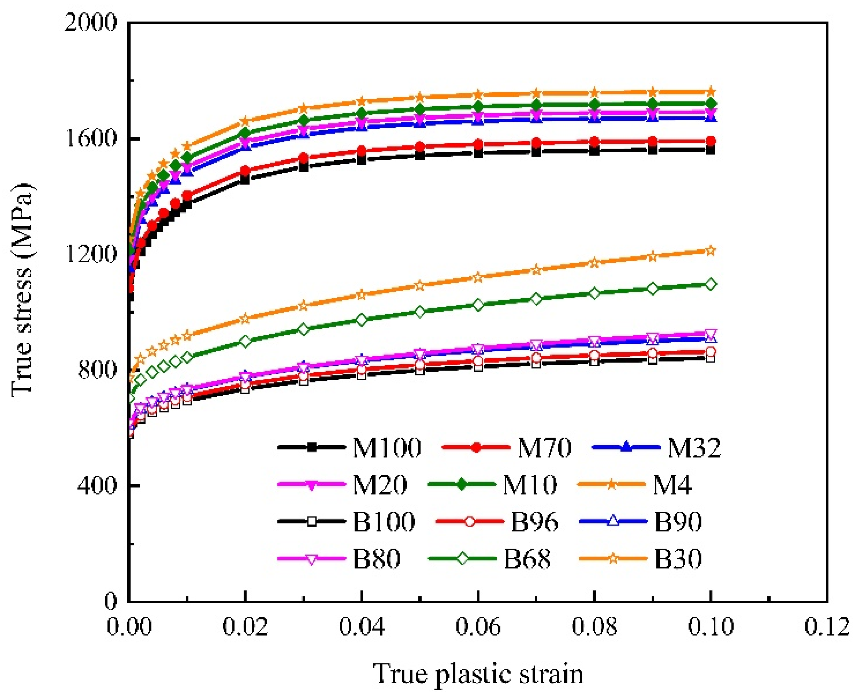
3.2.2. Constitutive Modeling of Individual Phases
3.2.3. Constitutive Modeling of Mixed B/M Microstructure
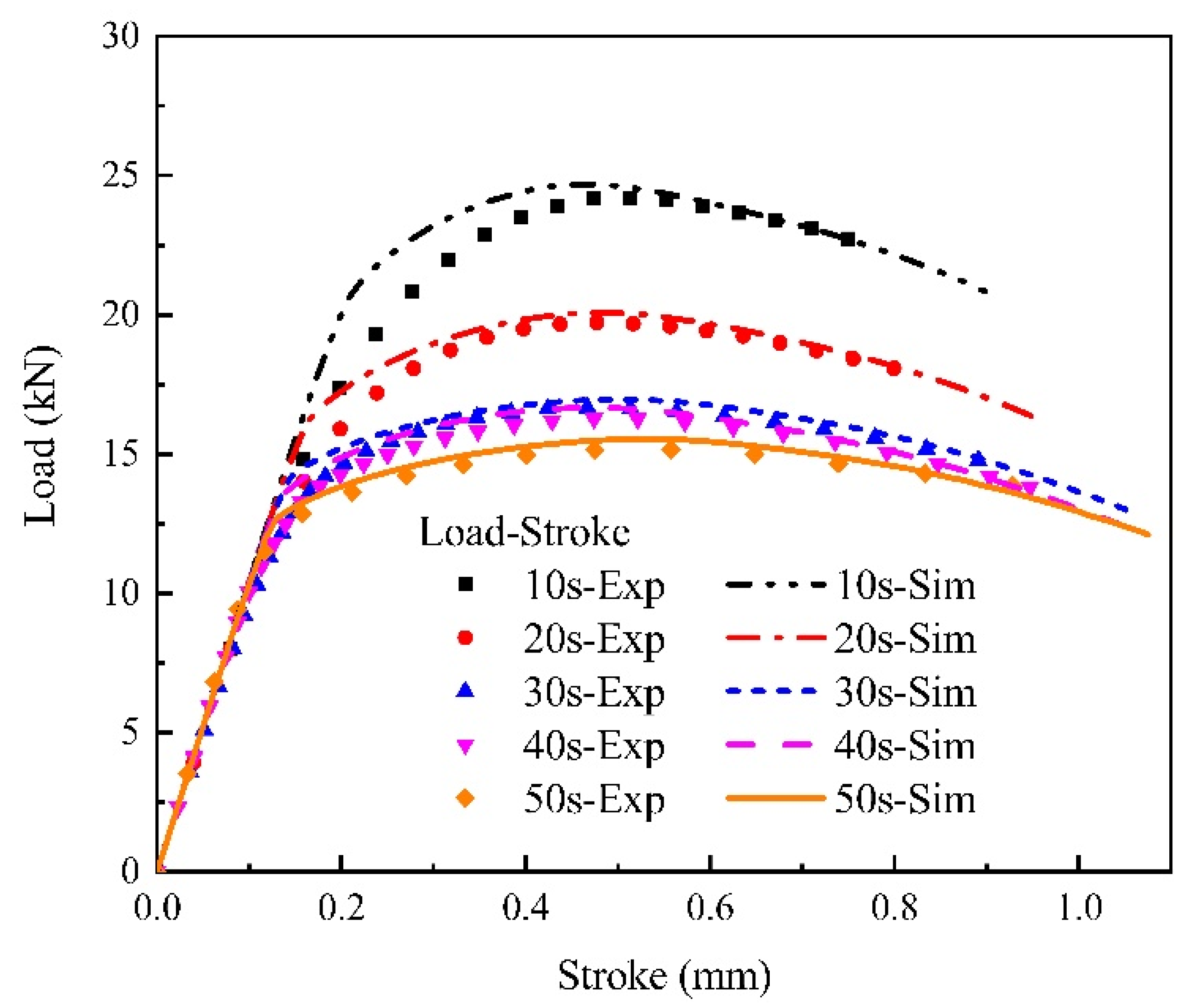
3.2.4. RVE Simulations for Uniaxial Tensile Specimens
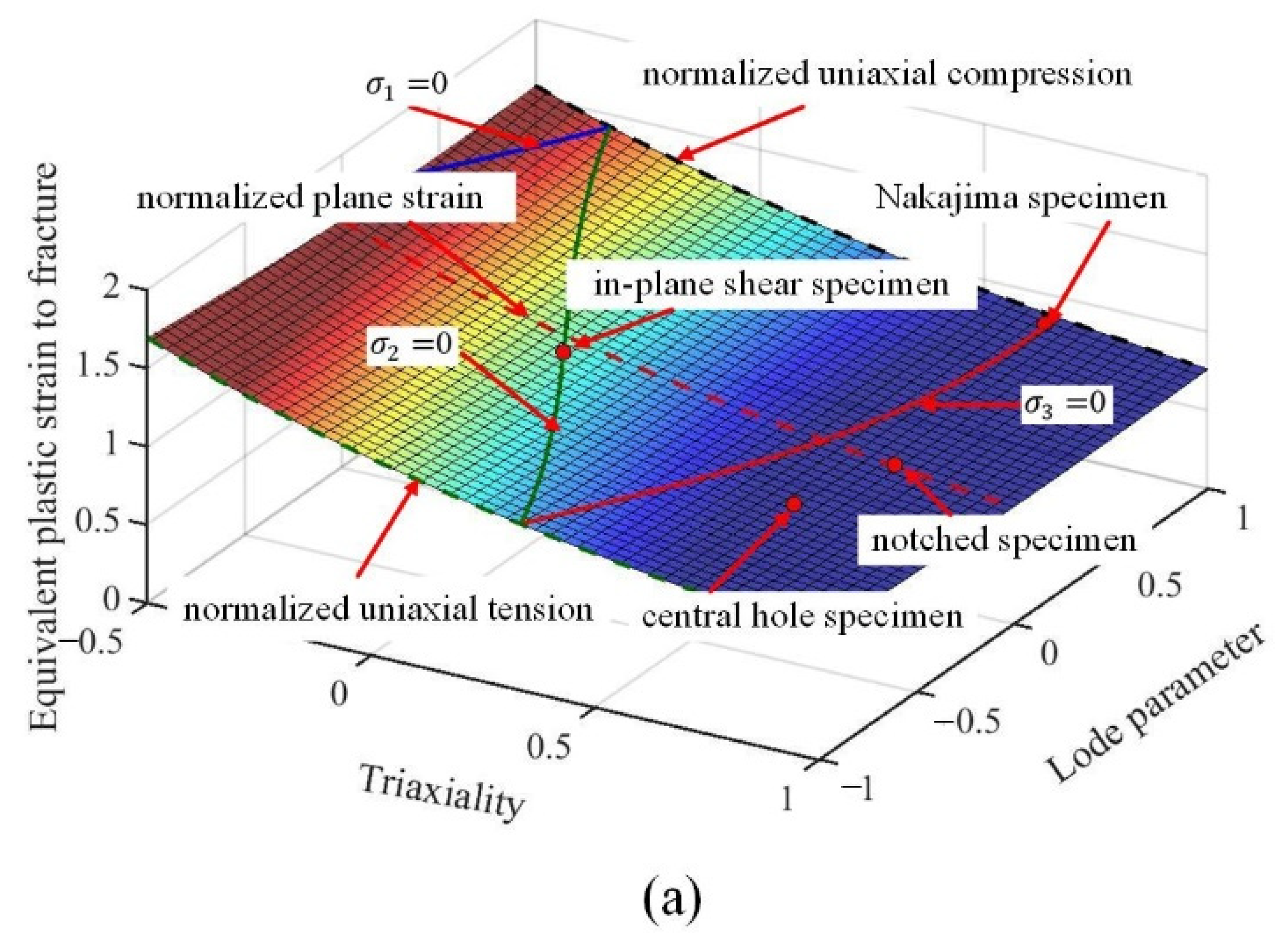
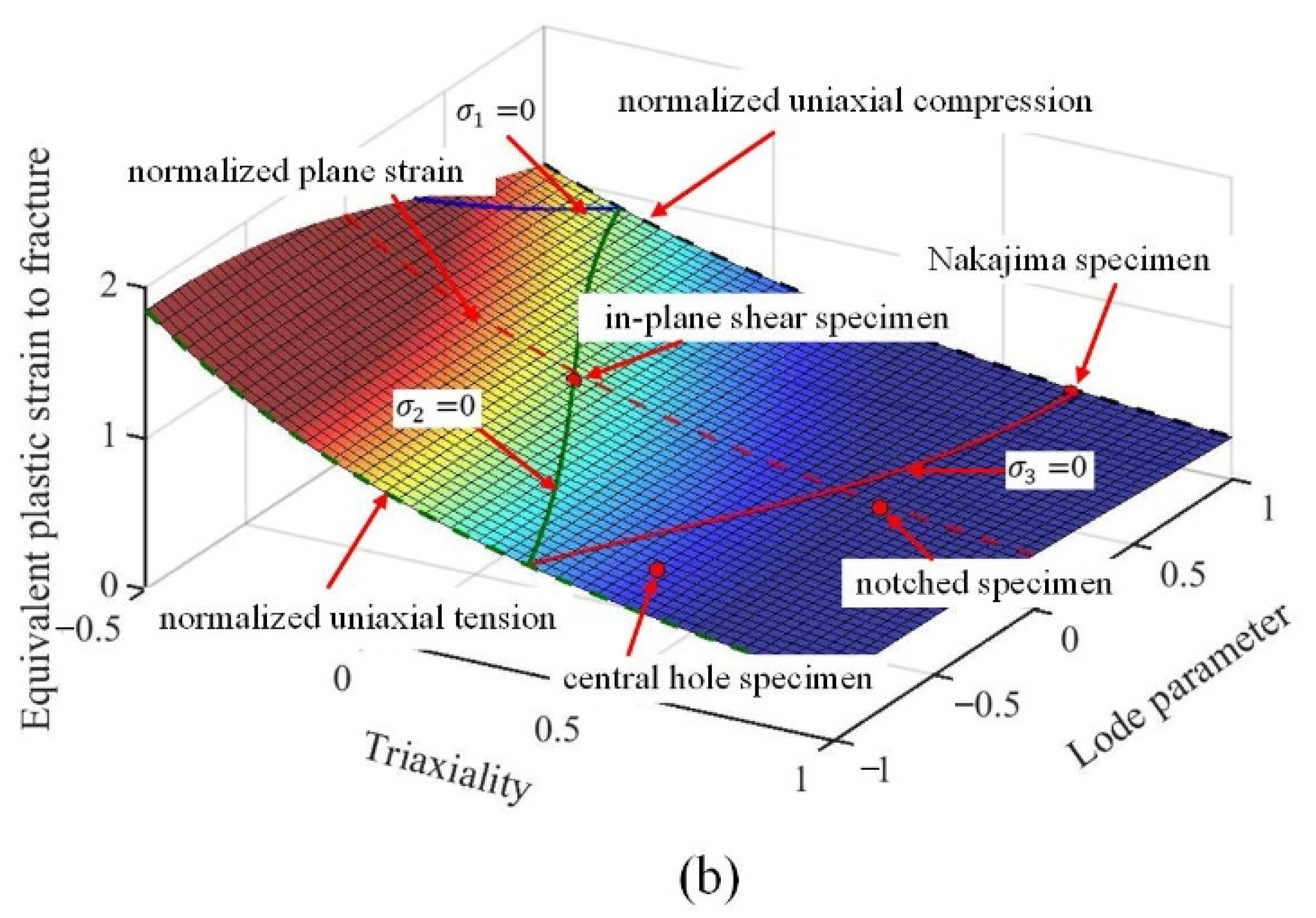
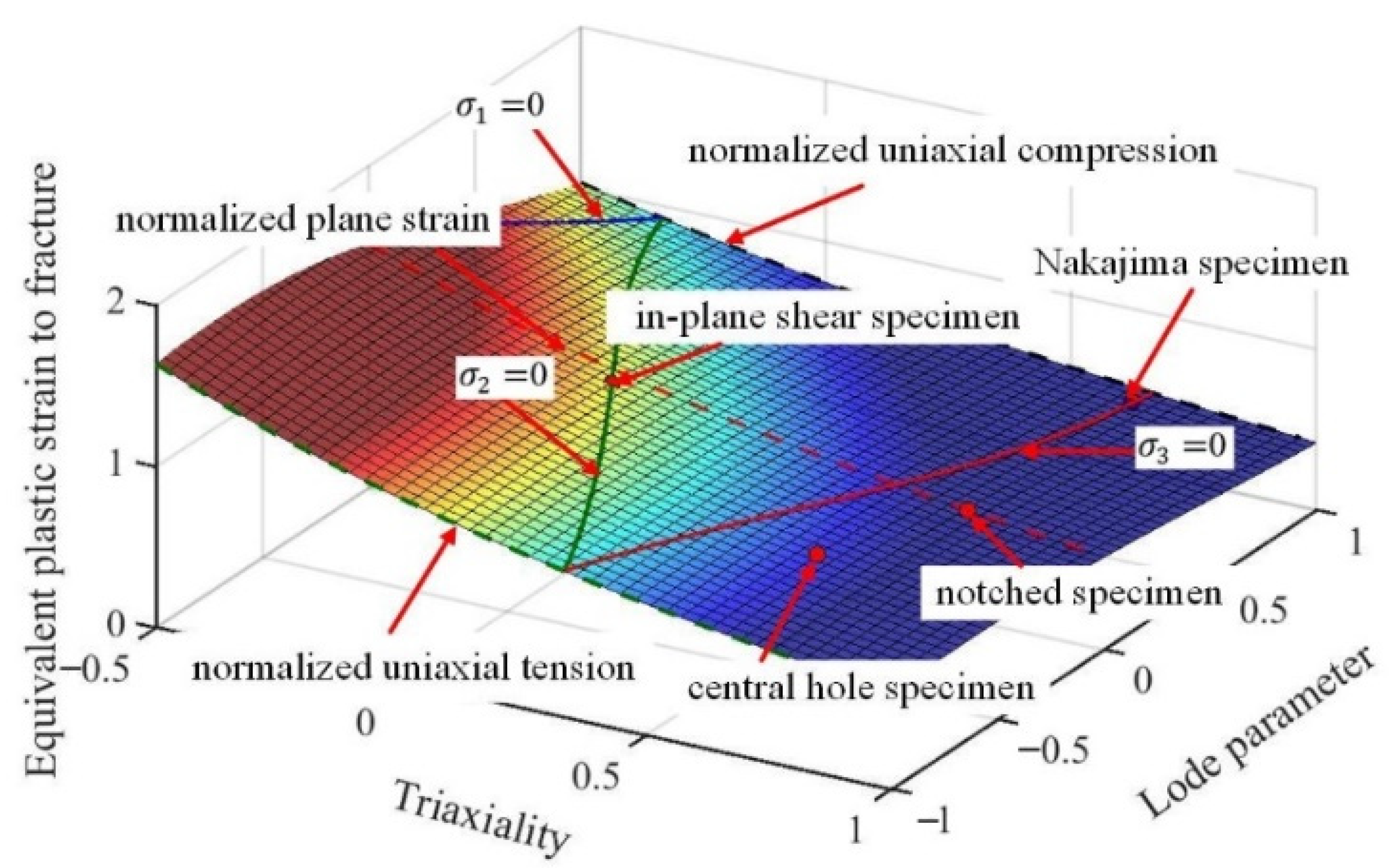
3.3. Damage Prediction
3.3.1. Damage Prediction of the Single Phase
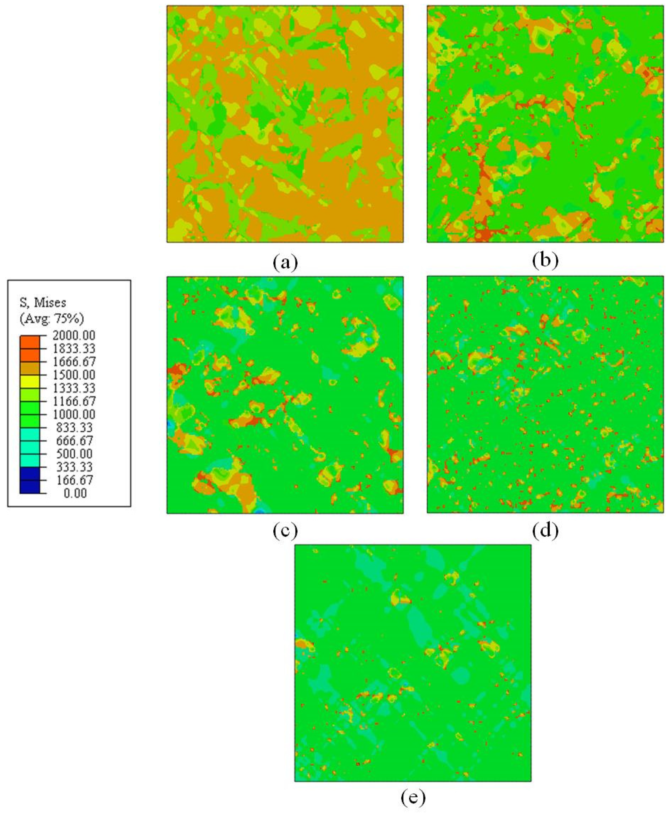
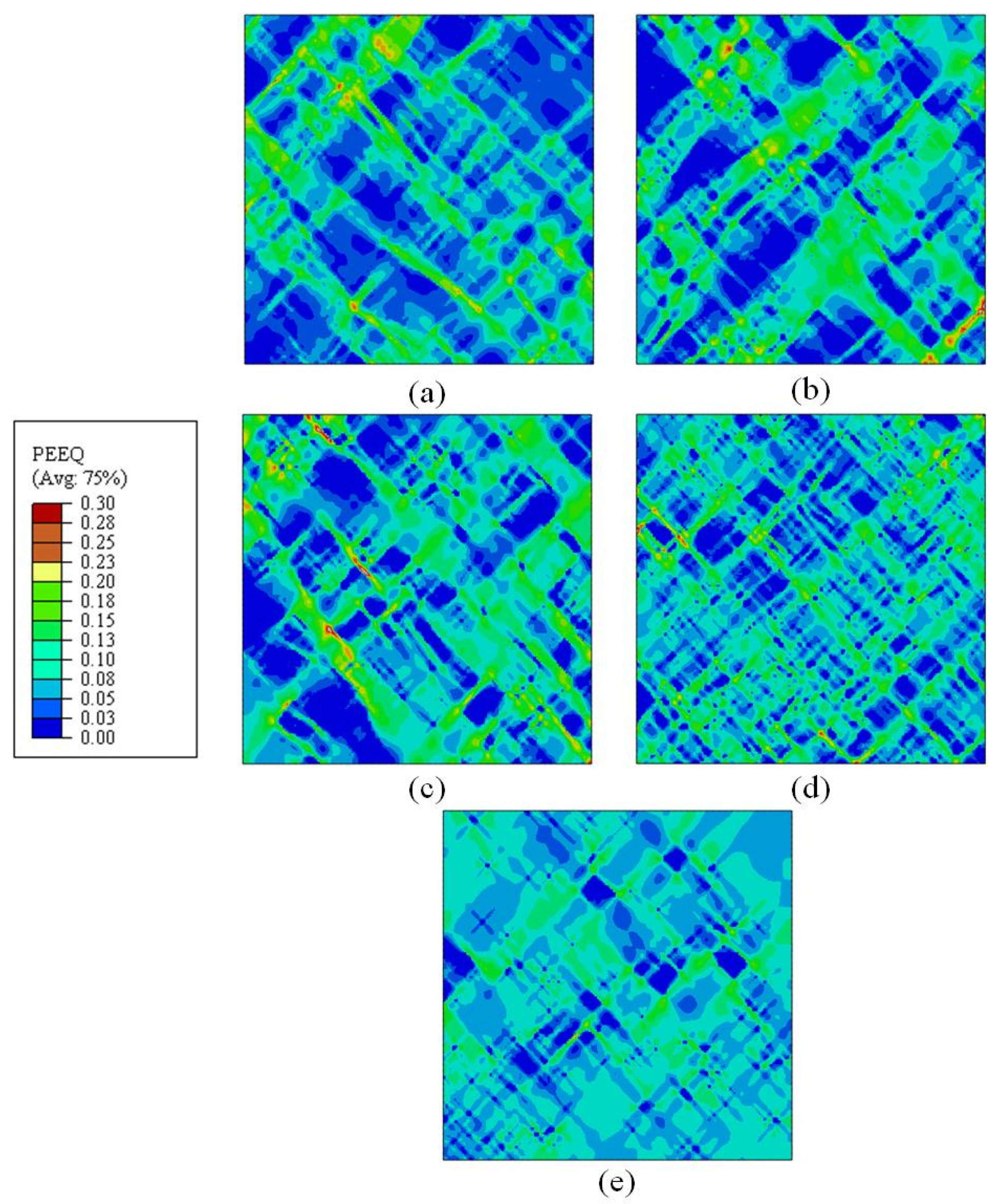
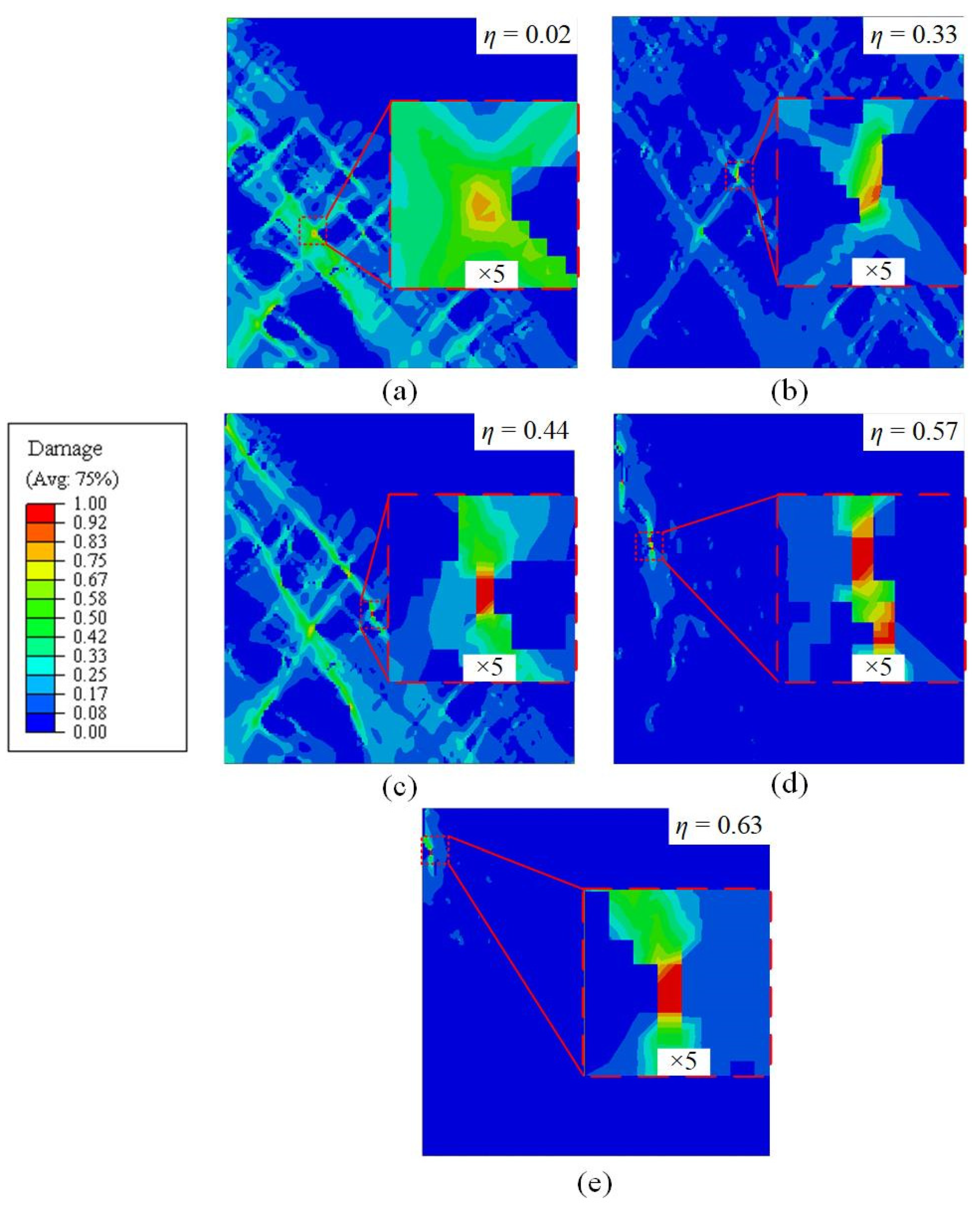
3.3.2. RVE Simulations in Varying Stress States
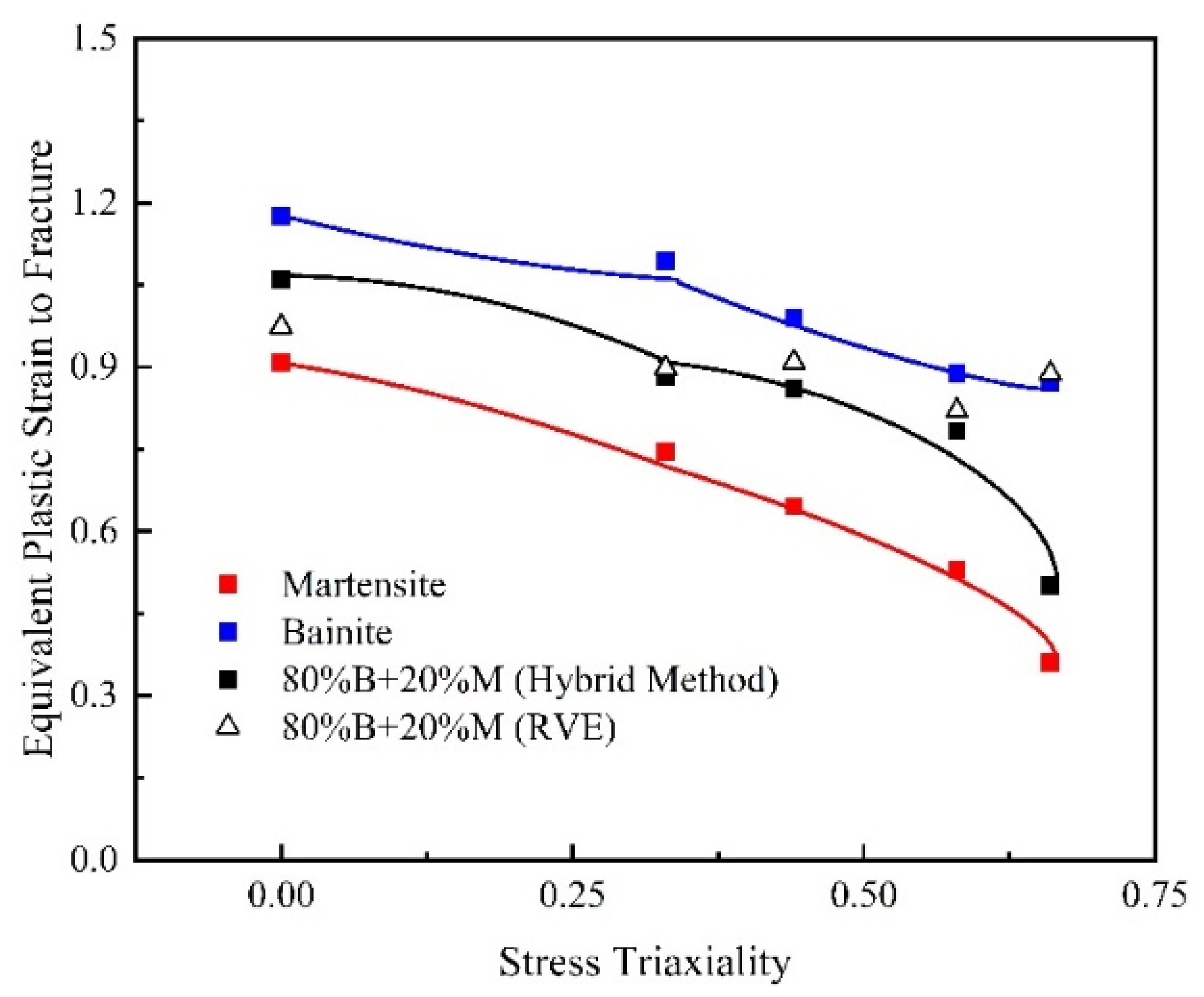
3.3.3. Damage Prediction of B/M Microstructures
4. Results and Discussion
5. Conclusions
Author Contributions
Funding
Institutional Review Board Statement
Data Availability Statement
Acknowledgments
Conflicts of Interest
Appendix A


References
- Merklein, M.; Wieland, M.; Lechner, M.; Bruschi, S.; Ghiotti, A. Hot stamping of boron steel sheets with tailored properties: A review. J. Mater. Proc. Technol. 2016, 228, 11–24. [Google Scholar] [CrossRef]
- Karbasian, H.; Tekkaya, A.E. A review on hot stamping. J. Mater. Proc. Technol. 2010, 210, 2103–2118. [Google Scholar] [CrossRef]
- Srithananan, P.; Kaewtatip, P.; Uthaisangsuk, V. Micromechanics-based modeling of stress–strain and fracture behavior of heat-treated boron steels for hot stamping process. Mater. Sci. Eng. A 2016, 667, 61–76. [Google Scholar] [CrossRef]
- Hein, P.; Wilsius, J. Status and innovation trends in hot stamping of USIBOR 1500 P. Steel Res. Int. 2008, 79, 85–91. [Google Scholar] [CrossRef]
- Maikranz-Valentin, M.; Weidig, U.; Schoof, U. Components with Optimised Properties due to Advanced Thermo-mechanical Process Strategies in Hot Sheet Metal Forming. Steel Res. Int. 2008, 79, 92–97. [Google Scholar] [CrossRef]
- Liang, W.; Wang, L.; Liu, Y.; Wang, Y.; Zhang, Y. Hot stamping parts with tailored properties by local resistance heating. Procedia Eng. 2014, 81, 1731–1736. [Google Scholar] [CrossRef]
- George, R.; Bardelcik, A.; Worswick, M.J. Hot forming of boron steels using heated and cooled tooling for tailored properties. J. Mater. Proc. Technol. 2012, 212, 2386–2399. [Google Scholar] [CrossRef]
- Cui, J.; Lei, C.; Xing, Z.; Li, C.; Ma, S. Predictions of the mechanical properties and microstructure evolution of high strength steel in hot stamping. J. Mater. Eng. Perform. 2012, 21, 2244–2254. [Google Scholar] [CrossRef]
- Cui, J.; Lei, C.; Xing, Z.; Li, C. Microstructure distribution and mechanical properties prediction of boron alloy during hot forming using FE simulation. Mater. Sci. Eng. A 2012, 535, 241–251. [Google Scholar] [CrossRef]
- Tang, B.T.; Bruschi, S.; Ghiotti, A.; Bariani, P. Numerical modelling of the tailored tempering process applied to 22MnB5 sheets. Finite Elem. Anal. Des. 2014, 81, 69–81. [Google Scholar] [CrossRef]
- Bardelcik, A.; Worswick, M.J.; Winkler, S.; Wells, M. A strain rate sensitive constitutive model for quenched boron steel with tailored properties. Int. J. Impact Eng. 2012, 50, 49–62. [Google Scholar] [CrossRef]
- Bardelcik, A.; Worswick, M.J.; Wells, M.A. The influence of martensite, bainite and ferrite on the as-quenched constitutive response of simultaneously quenched and deformed boron steel–Experiments and model. Mater. Des. 2014, 55, 509–525. [Google Scholar] [CrossRef]
- Eller, T.K.; Greve, L.; Andres, M.T.; Medricky, M.; Hatscher, A.; Meinders, V.; Boogaard, T.V.D. Plasticity and fracture modeling of quench-hardenable boron steel with tailored properties. J. Mater. Proc. Technol. 2014, 214, 1211–1227. [Google Scholar] [CrossRef]
- Mohr, D.; Ebnoether, F. Plasticity and fracture of martensitic boron steel under plane stress conditions. Int. J. Solids Struct 2009, 46, 3535–3547. [Google Scholar] [CrossRef][Green Version]
- Tang, B.; Wu, F.; Wang, Q.; Liu, J.; Guo, N.; Ge, H.; Wang, Q.; Liu, P. Damage prediction of hot stamped boron steel 22MnB5 with a microscopic motivated ductile fracture criterion: Experiment and simulation. Int. J. Mech. Sci. 2020, 169, 105302. [Google Scholar] [CrossRef]
- Tang, B.; Wu, F.; Wang, Q.; Li, C.; Liu, J.; Ge, H. Numerical and experimental study on ductile fracture of quenchable boron steels with different microstructures. Int. J. Lightweight Mater. Manuf. 2020, 3, 55–65. [Google Scholar] [CrossRef]
- Sodjit, S.; Uthaisangsuk, V. Microstructure based prediction of strain hardening behavior of dual phase steels. Mater. Des. 2012, 41, 370–379. [Google Scholar] [CrossRef]
- Phetlam, P.; Uthaisangsuk, V. Microstructure based flow stress modeling for quenched and tempered low alloy steel. Mater. Des. 2015, 82, 189–199. [Google Scholar] [CrossRef]
- Anbarlooie, B.; Hosseini-Toudeshky, H.; Hosseini, M.; Kadkhodapour, J. Experimental and 3D micromechanical analysis of stress–strain behavior and damage initiation in dual-phase steels. J. Mater. Eng. Perform. 2019, 28, 2903–2918. [Google Scholar] [CrossRef]
- Ramazani, A.; Mukherjee, K.; Quade, H.; Prahl, U.; Bleck, W. Correlation between 2D and 3D flow curve modelling of DP steels using a microstructure-based RVE approach. Mater. Sci. Eng. A 2013, 560, 129–139. [Google Scholar] [CrossRef]
- Golling, S.; Frómeta, D.; Casellas, D.; Jonsén, P. Influence of microstructure on the fracture toughness of hot stamped boron steel. Mater. Sci. Eng. A 2019, 743, 529–539. [Google Scholar] [CrossRef]
- Lian, J.; Yang, H.; Vajragupta, N.; Münstermann, S.; Bleck, W. A method to quantitatively upscale the damage initiation of dual-phase steels under various stress states from microscale to macroscale. Comp. Mater. Sci 2014, 94, 245–257. [Google Scholar] [CrossRef]
- Toda, H.; Takijiri, A.; Azuma, M.; Yabu, S.; Hayashi, K.; Seo, D.; Kobayashi, M.; Hirayama, K.; Takeuchi, A.; Uesugi, K. Damage micromechanisms in dual-phase steel investigated with combined phase-and absorption-contrast tomography. Acta Mater. 2017, 126, 401–412. [Google Scholar] [CrossRef]
- Hoefnagels, J.P.M.; Tasan, C.C.; Maresca, F.; Peters, F.J.; Kouznetsova, V. Retardation of plastic instability via damage-enabled microstrain delocalization. J. Mater. Sci. 2015, 50, 6882–6897. [Google Scholar] [CrossRef]
- Tang, A.; Liu, H.; Chen, R.; Liu, G.; Lai, Q.; Zhong, Y.; Wang, L.; Wang, J.; Lu, Q.; Shen, Y. Mesoscopic origin of damage nucleation in dual-phase steels. Int. J. Plast. 2021, 137, 102920. [Google Scholar] [CrossRef]
- Matsuno, T.; Maeda, D.; Shutoh, H.; Uenishi, A.; Suehiro, M. Effect of martensite volume fraction on void formation leading to ductile fracture in dual phase steels. ISIJ Int. 2014, 54, 938–944. [Google Scholar] [CrossRef]
- Ismail, K.; Perlade, A.; Jacques, P.J.; Pardoen, T.; Brassart, L. Impact of second phase morphology and orientation on the plastic behavior of dual-phase steels. Int. J. Plast. 2019, 118, 130–146. [Google Scholar] [CrossRef]
- Zhang, J.; Di, H.; Deng, Y.; Misra, R. Effect of martensite morphology and volume fraction on strain hardening and fracture behavior of martensite–ferrite dual phase steel. Mater. Sci. Eng. A 2015, 627, 230–240. [Google Scholar] [CrossRef]
- Avramovic-Cingara, G.; Ososkov, Y.; Jain, M.K.; Wilkinson, D. Effect of martensite distribution on damage behaviour in DP600 dual phase steels. Mater. Sci. Eng. A 2009, 516, 7–16. [Google Scholar] [CrossRef]
- Calcagnotto, M.; Adachi, Y.; Ponge, D.; Raabe, D. Deformation and fracture mechanisms in fine-and ultrafine-grained ferrite/martensite dual-phase steels and the effect of aging. Acta Mater. 2011, 59, 658–670. [Google Scholar] [CrossRef]
- Yan, D.; Tasan, C.C.; Raabe, D. High resolution in situ mapping of microstrain and microstructure evolution reveals damage resistance criteria in dual phase steels. Acta Mater. 2015, 96, 399–409. [Google Scholar] [CrossRef]
- Saeidi, N.; Ashrafizadeh, F.; Niroumand, B.; Forouzan, M.; Mofidi, S.M.; Barlat, F. Examination and modeling of void growth kinetics in modern high strength dual phase steels during uniaxial tensile deformation. Mater. Chem. Phys. 2016, 172, 54–61. [Google Scholar] [CrossRef]
- Matsuno, T.; Teodosiu, C.; Maeda, D.; Uenishi, A. Mesoscale simulation of the early evolution of ductile fracture in dual-phase steels. Int. J. Plast 2015, 74, 17–34. [Google Scholar] [CrossRef]
- Avramovic-Cingara, G.; Saleh, C.A.R.; Jain, M.K.; Wilkinson, D. Void nucleation and growth in dual-phase steel 600 during uniaxial tensile testing. Metall. Mater. Trans. 2009, 40, 3117–3127. [Google Scholar] [CrossRef]
- Tang, B.; Wang, Q.; Guo, N.; Liu, J.; Ge, H.; Luo, Z.; Li, X. Microstructure-based RVE modeling of ductile failure induced by plastic strain localization in tailor-tempered 22MnB5 boron steel. Eng. Fract. Mech. 2020, 240, 107351. [Google Scholar] [CrossRef]
- Evening, M.; Schewe, J. Adobe Photoshop CS5 for Photographers: The Ultimate Workshop; Routledge: Abingdon-on-Thames, UK, 2012. [Google Scholar]
- Roth, C.C.; Mohr, D. Effect of strain rate on ductile fracture initiation in advanced high strength steel sheets: Experiments and modeling. Int. J. Plast. 2014, 56, 19–44. [Google Scholar] [CrossRef]
- Tang, B.; Wu, F.; Guo, N.; Liu, J.; Ge, H.; Bruschi, S.; Li, X. Numerical modeling of ductile fracture of hot stamped 22MnB5 boron steel parts in three-point bending. Int. J. Mech. Sci. 2020, 188, 105951. [Google Scholar] [CrossRef]
- Reid, A.C.E.; Lua, R.C.; García, R.E.; Coffman, V.R.; Langer, S.A. Modelling microstructures with OOF2. Int. J. Mater. Product Technol. 2009, 35, 361–373. [Google Scholar] [CrossRef]
- Ramazani, A.; Mukherjee, K.; Prahl, U.; Bleck, W. Transformation-induced, geometrically necessary, dislocation-based flow curve modeling of dual-phase steels: Effect of grain size. Metall Mater. Trans. A 1985, 43, 3850–3869. [Google Scholar] [CrossRef]
- Rodriguez, R.M.; Gutierrez, I. Unified formulation to predict the tensile curves of steels with different microstructures. Mater. Sci. Forum. 2003, 426–432, 4525–4530. [Google Scholar] [CrossRef]
- Rodriguez, R.M.; Gutierrez, I. Mechanical behaviour of steels with mixed microstructures. Proc. TMP 2004, 4, 356–363. [Google Scholar]
- Luo, M.; Dunand, M.; Mohr, D. Experiments and modeling of anisotropic aluminum extrusions under multi-axial loading–Part II: Ductile fracture. Int. J. Plast. 2012, 32, 36–58. [Google Scholar] [CrossRef]
- Golling, S.; Östlund, R.; Oldenburg, M. A study on homogenization methods for steels with varying content of ferrite, bainite and martensite. J. Mater. Proc. Technol. 2016, 228, 88–97. [Google Scholar] [CrossRef]
- Zhang, C.; Wang, Y.; Chen, Z.; Yang, N.; Lou, Y.; Clausmeyer, T.; Tekkaya, A.E.; Zhang, Q. Characterization of plasticity and fracture of an QP1180 steel sheet. Procedia Manuf. 2020, 50, 529–534. [Google Scholar] [CrossRef]
- Lou, Y.; Huh, H. Prediction of ductile fracture for advanced high strength steel with a new criterion: Experiments and simulation. J. Mater. Proc. Technol. 2013, 213, 1284–1302. [Google Scholar] [CrossRef]
- Lou, Y.; Chen, L.; Clausmeyer, T.; Tekkaya, A.E.; Yoon, J.W. Modeling of ductile fracture from shear to balanced biaxial tension for sheet metals. Int. J. Solids Struct. 2017, 112, 169–184. [Google Scholar] [CrossRef]
- Dunand, M.; Mohr, D. Hybrid experimental–numerical analysis of basic ductile fracture experiments for sheet metals. Int. J. Solids Struct. 2010, 47, 1130–1143. [Google Scholar] [CrossRef]
- Darabi, A.C.; Kadkhodapour, J.; Anaraki, A.P.; Khoshbin, M.; Alaie, A.; Schmauder, S. Micromechanical modeling of damage mechanisms in dual-phase steel under different stress states. Eng. Fract. Mech. 2021, 243, 107520. [Google Scholar] [CrossRef]


| C | Si | Mn | P | S | Cr | Ti | B |
|---|---|---|---|---|---|---|---|
| 0.21 | 0.25 | 1.34 | 0.009 | 0.006 | 0.20 | 0.03 | 0.002 |
| Time (s) | Modified LePera | SEM | ||
|---|---|---|---|---|
| Martensite (%) | Bainite (%) | Martensite (%) | Bainite (%) | |
| 10 | 70 | 30 | 64 | 36 |
| 20 | 32 | 68 | 34 | 66 |
| 30 | 20 | 80 | 18 | 82 |
| 40 | 10 | 90 | 12 | 88 |
| 50 | 4 | 96 | 5 | 95 |
| Dogbone | Central Hole | Notched | In-Plane Shear | Nakajima |
|---|---|---|---|---|
| 1.8 | 0.3 | 0.5 | 0.5 | 30 |
| Phase | (m) | k | ||||||
|---|---|---|---|---|---|---|---|---|
| Bainite | 218.29 | 360.97 | 0.33 | 3 | 80 | 5.75 | ||
| Martensite | 218.29 | 834.73 | 0.33 | 3 | 80 | 16.75 |
| Phase Fraction | k | ||
|---|---|---|---|
| B30 | 555.4 | 0.644 | |
| B68 | 484.8 | 1.958 | |
| B80 | 400.4 | 2.7 | |
| B90 | 390.4 | 4.4 | |
| B96 | 370.4 | 5.6 |
| Phase Fraction | k | ||
|---|---|---|---|
| M4 | 1034.73 | 16.75 | |
| M10 | 994.73 | 16.75 | |
| M20 | 964.73 | 16.75 | |
| M32 | 934.73 | 16.75 | |
| M70 | 864.73 | 16.75 |
| Specimen | Lode Parameter | Lode Angle | Normalized Lode Angle | Stress Triaxiality | Fracture Strain |
|---|---|---|---|---|---|
| Central hole | −0.4775 | 0.2546 | 0.5138 | 0.7169 | 0.9901 |
| Notched R5 | −0.0458 | 0.4972 | 0.0505 | 0.7527 | 0.8896 |
| In-plane shear | −0.0945 | 0.4691 | 0.1041 | 0.0365 | 1.1766 |
| Nakajima | 0.9469 | 1.0239 | −0.9555 | 0.6603 | 0.8719 |
| Specimen | Lode Parameter | Lode Angle | Normalized Lode Angle | Stress Triaxiality | Fracture Strain |
|---|---|---|---|---|---|
| Central hole | −0.8030 | 0.0895 | 0.8291 | 0.5290 | 0.6458 |
| Notched R5 | −0.0537 | 0.4926 | 0.0592 | 0.6892 | 0.5155 |
| In-plane shear | −0.0517 | 0.4937 | 0.0570 | 0.0211 | 0.9076 |
| Nakajima | 0.9780 | 1.0376 | −0.9817 | 0.6578 | 0.3612 |
| Stress Triaxiality | |||
|---|---|---|---|
| 100 | −80 | −0.8 | 0.02 |
| 100 | 0 | 0 | 0.33 |
| 100 | 18 | 0.18 | 0.44 |
| 100 | 60 | 0.6 | 0.57 |
| 100 | 100 | 1 | 0.63 |
| Specimen | Lode Parameter | Lode Angle | Normalized Lode Angle | Stress Triaxiality | Fracture Strain |
|---|---|---|---|---|---|
| Central hole | −0.5738 | 0.2037 | 0.6110 | 0.6635 | 0.8608 |
| Notched R5 | −0.0465 | 0.4968 | 0.0513 | 0.7549 | 0.7835 |
| In-plane shear | −0.0766 | 0.4794 | 0.0844 | 0.0294 | 1.0672 |
| Nakajima | 0.9243 | 1.0138 | −0.9362 | 0.6564 | 0.5019 |
Publisher’s Note: MDPI stays neutral with regard to jurisdictional claims in published maps and institutional affiliations. |
© 2022 by the authors. Licensee MDPI, Basel, Switzerland. This article is an open access article distributed under the terms and conditions of the Creative Commons Attribution (CC BY) license (https://creativecommons.org/licenses/by/4.0/).
Share and Cite
Zhang, H.; Liu, G.; Guo, N.; Meng, X.; Shi, Y.; Su, H.; Liu, Z.; Tang, B. Damage Evolution of Hot Stamped Boron Steels Subjected to Various Stress States: Macro/Micro-Scale Experiments and Simulations. Materials 2022, 15, 1751. https://doi.org/10.3390/ma15051751
Zhang H, Liu G, Guo N, Meng X, Shi Y, Su H, Liu Z, Tang B. Damage Evolution of Hot Stamped Boron Steels Subjected to Various Stress States: Macro/Micro-Scale Experiments and Simulations. Materials. 2022; 15(5):1751. https://doi.org/10.3390/ma15051751
Chicago/Turabian StyleZhang, Hao, Guoqiang Liu, Ning Guo, Xiangbin Meng, Yanbin Shi, Hangqi Su, Zhe Liu, and Bingtao Tang. 2022. "Damage Evolution of Hot Stamped Boron Steels Subjected to Various Stress States: Macro/Micro-Scale Experiments and Simulations" Materials 15, no. 5: 1751. https://doi.org/10.3390/ma15051751
APA StyleZhang, H., Liu, G., Guo, N., Meng, X., Shi, Y., Su, H., Liu, Z., & Tang, B. (2022). Damage Evolution of Hot Stamped Boron Steels Subjected to Various Stress States: Macro/Micro-Scale Experiments and Simulations. Materials, 15(5), 1751. https://doi.org/10.3390/ma15051751