
Artificial Neural Networks for Predicting Plastic Anisotropy of Sheet Metals Based on Indentation Test


Abstract
:
1. Introduction
2. Materials and Methods
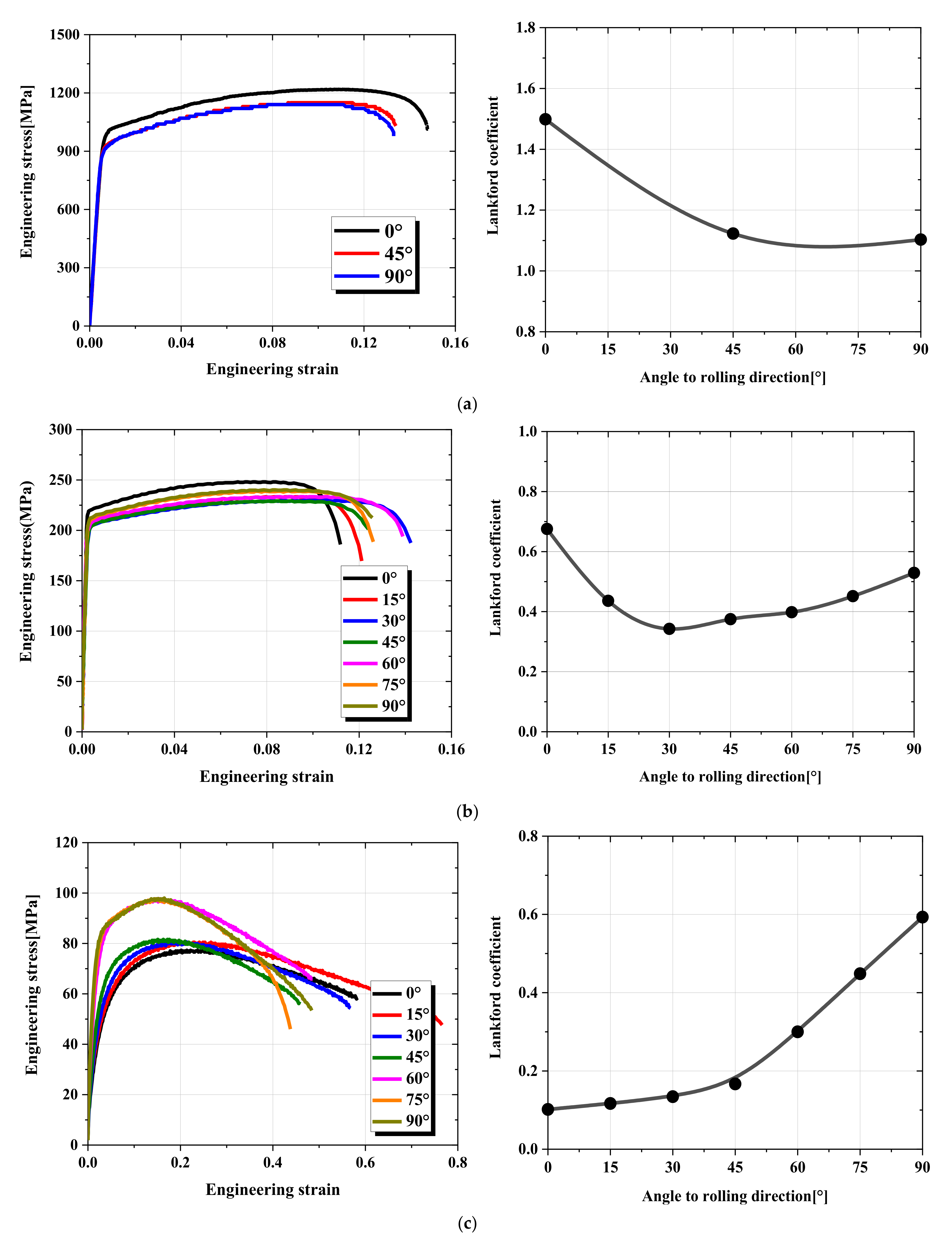
2.1. Mechanical Property Measurement of Materials
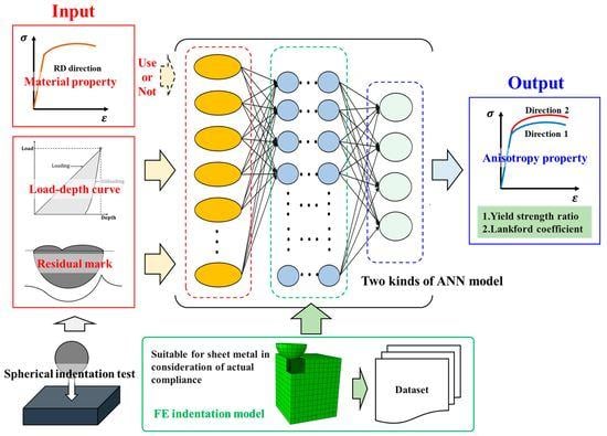
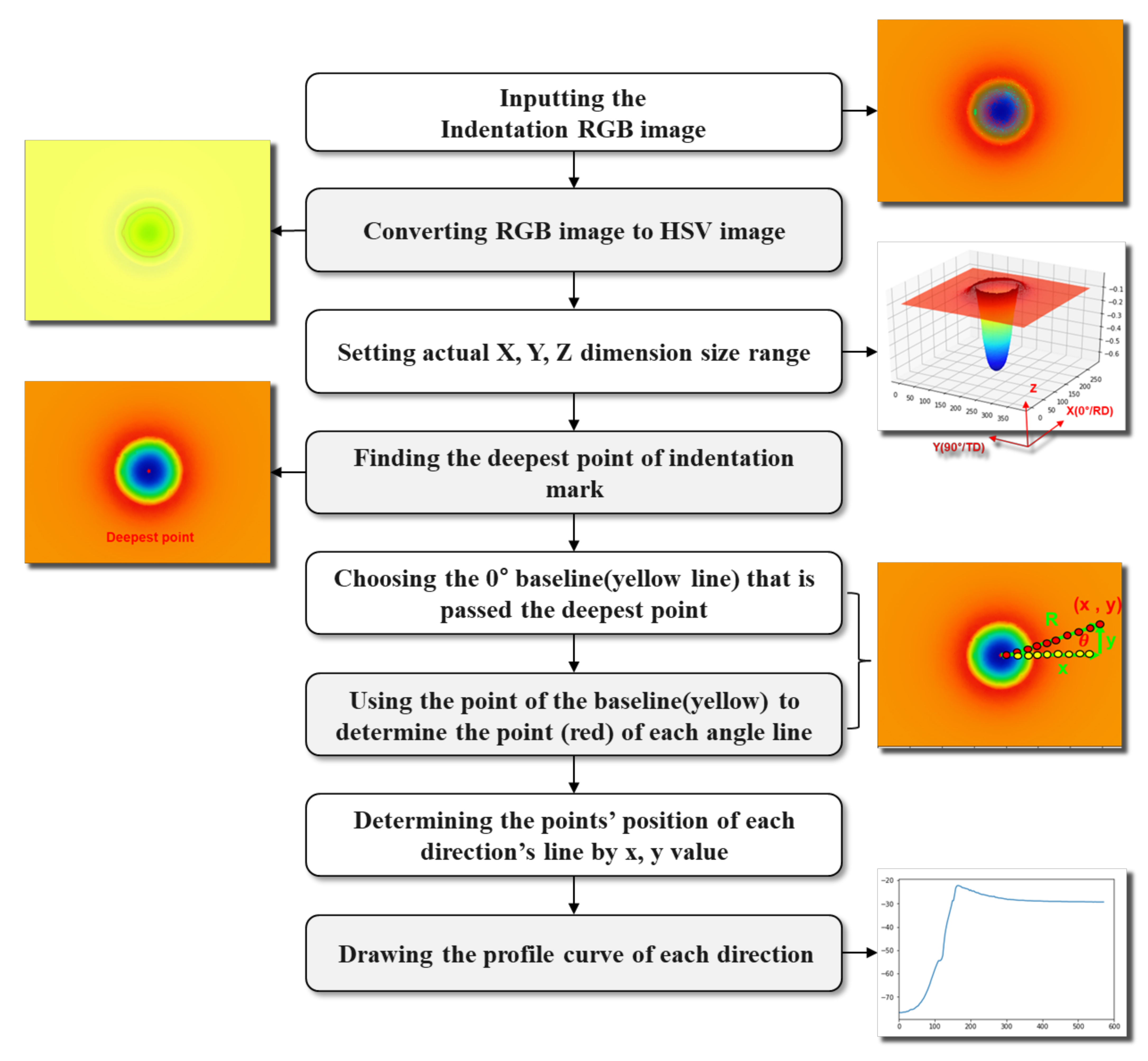
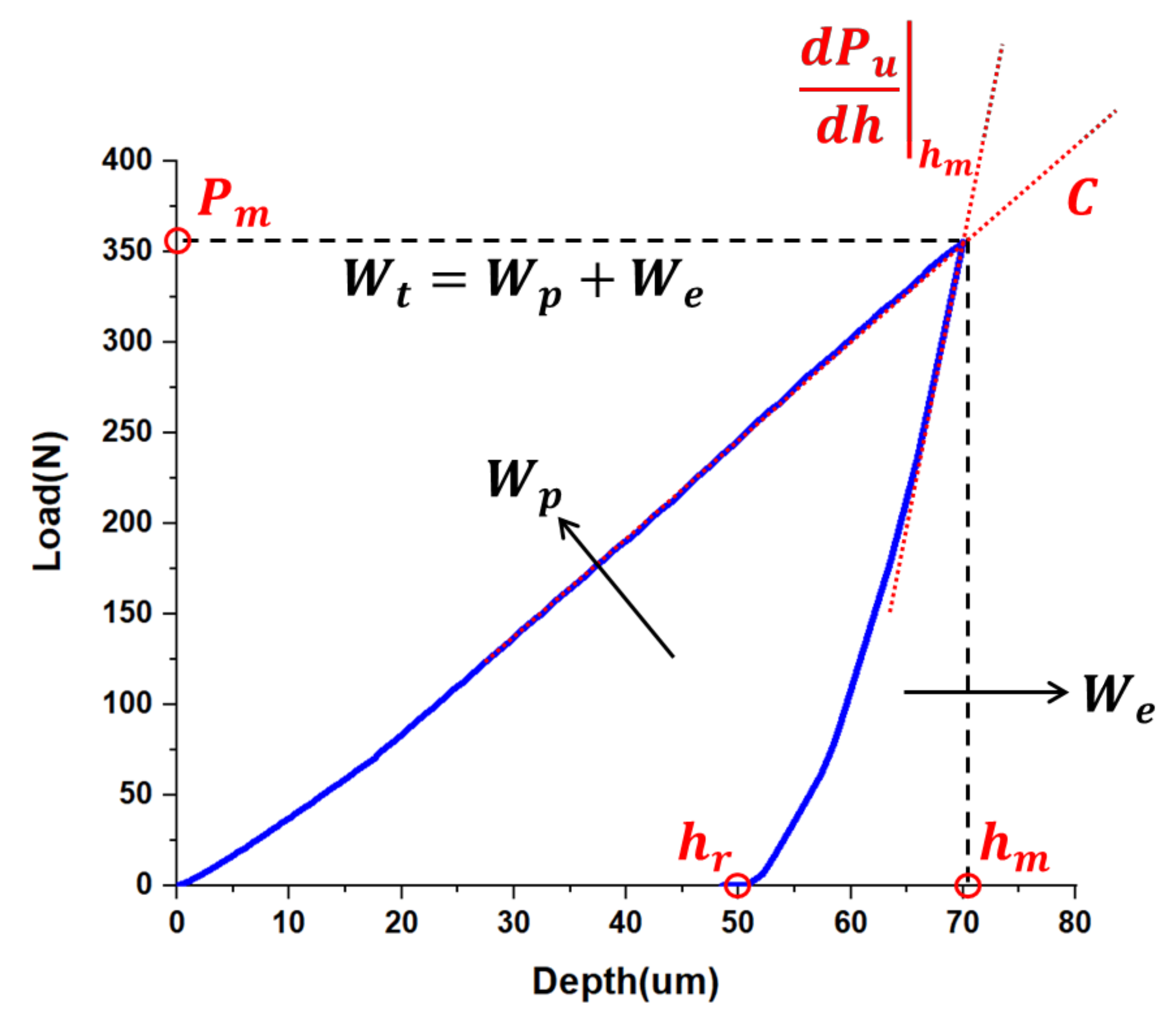
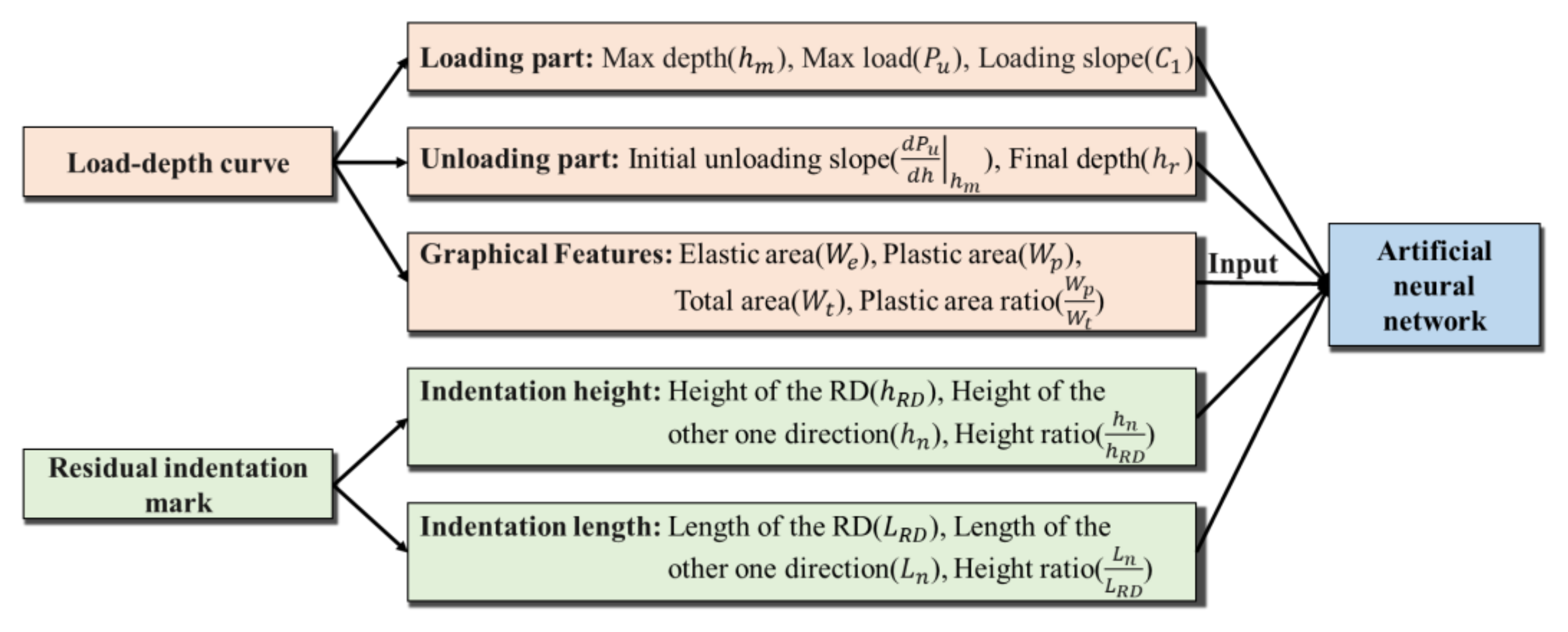
2.2. Input Parameters for the Proposed ANN Model
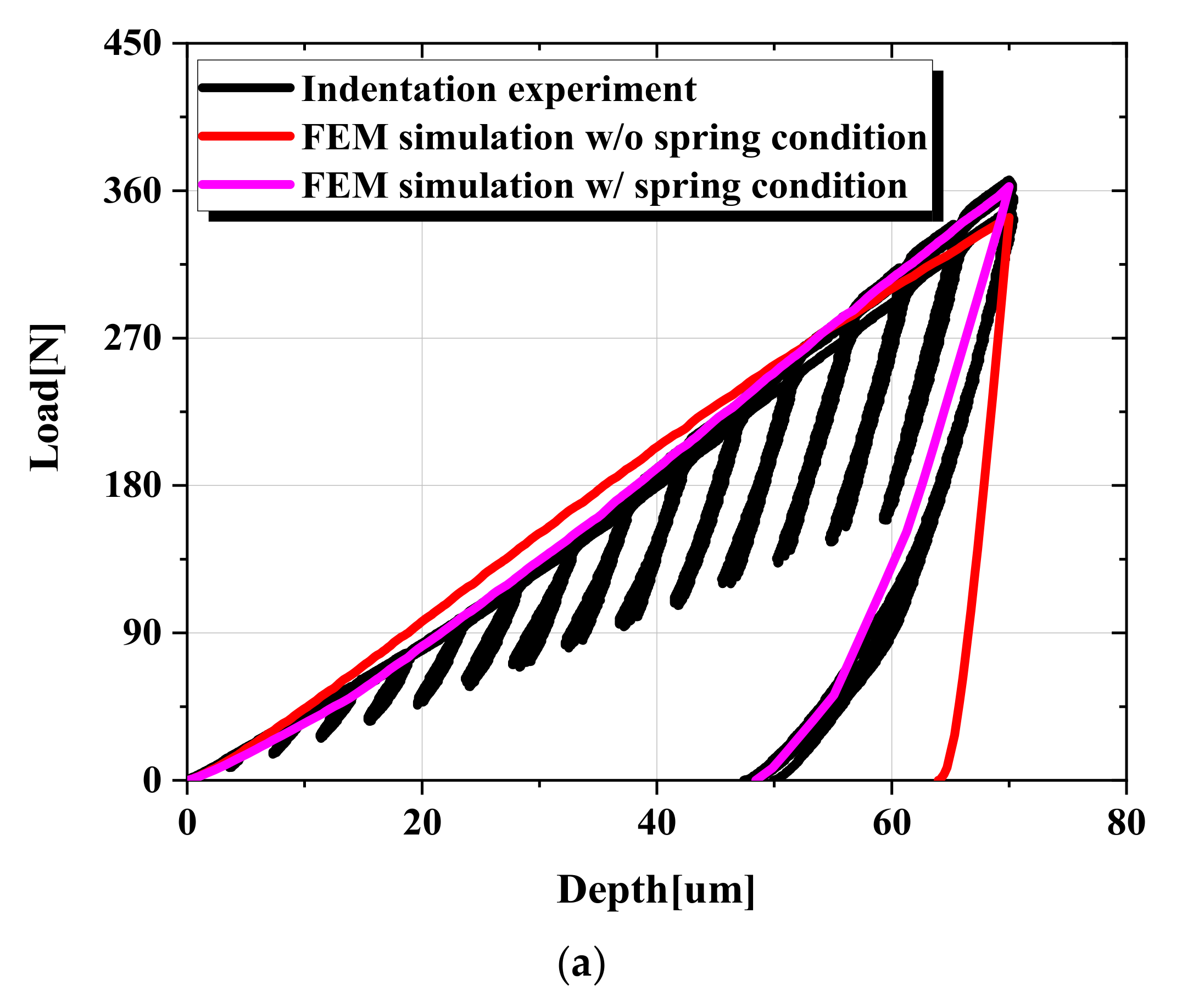
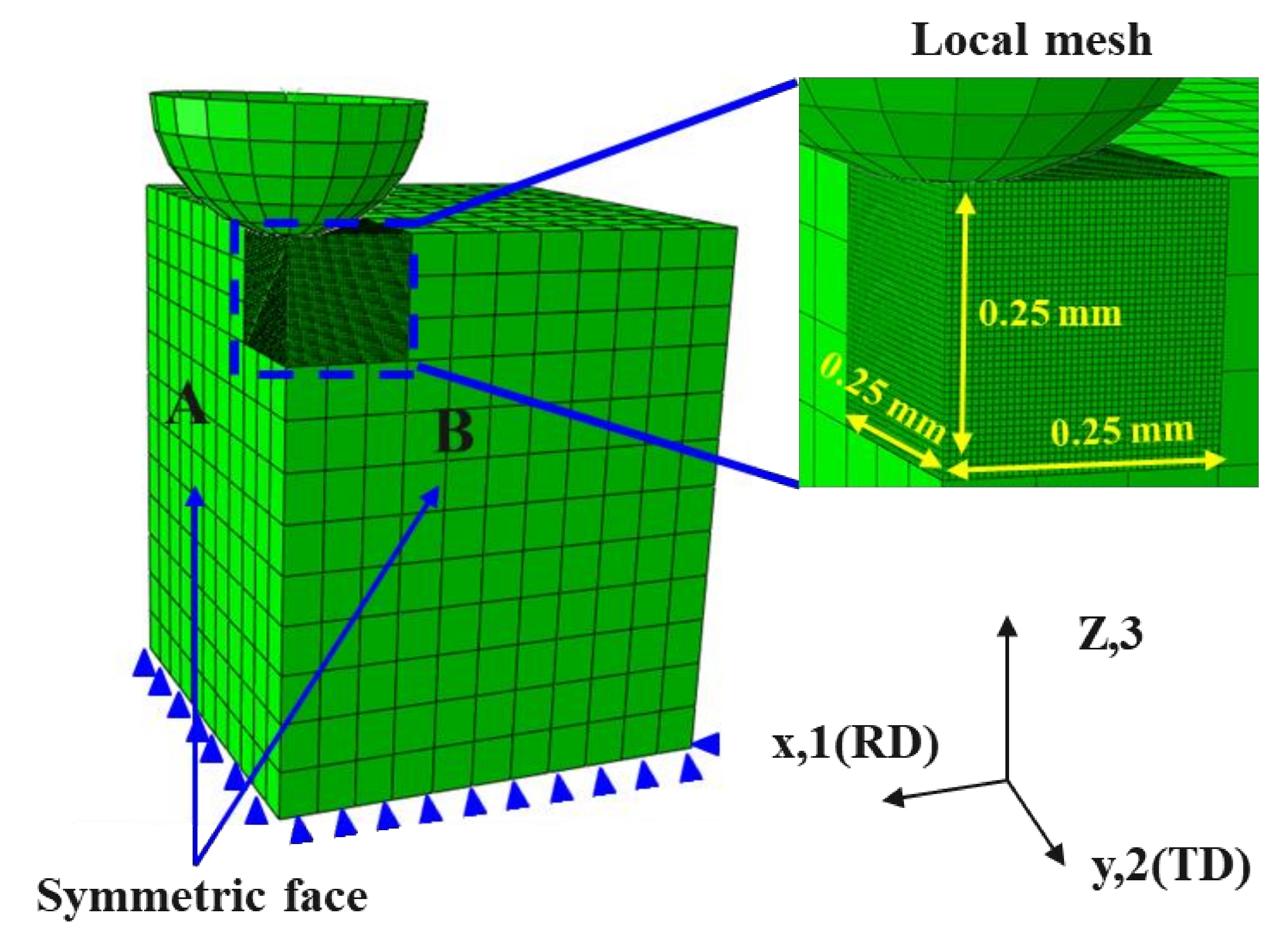
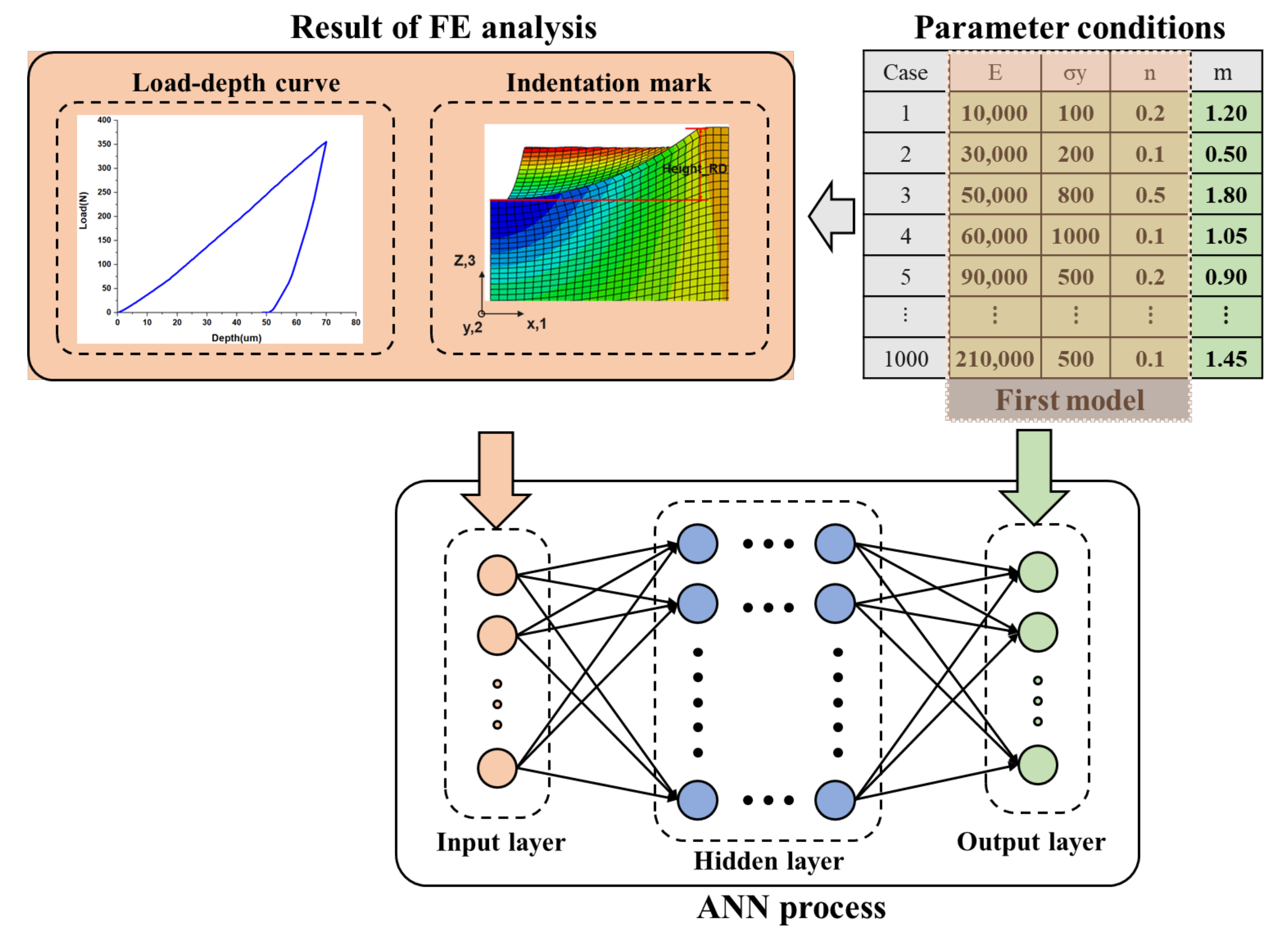
2.3. Dataset Acquisition Using FE Model for ANN Model
2.4. Anisotropy Artificial Neural Network Model
3. Results
4. Conclusions
- An ANN model for predicting anisotropic properties of materials was constructed, and this model can replace the conventional dimensionless analysis with complex procedures to derive the analysis function.
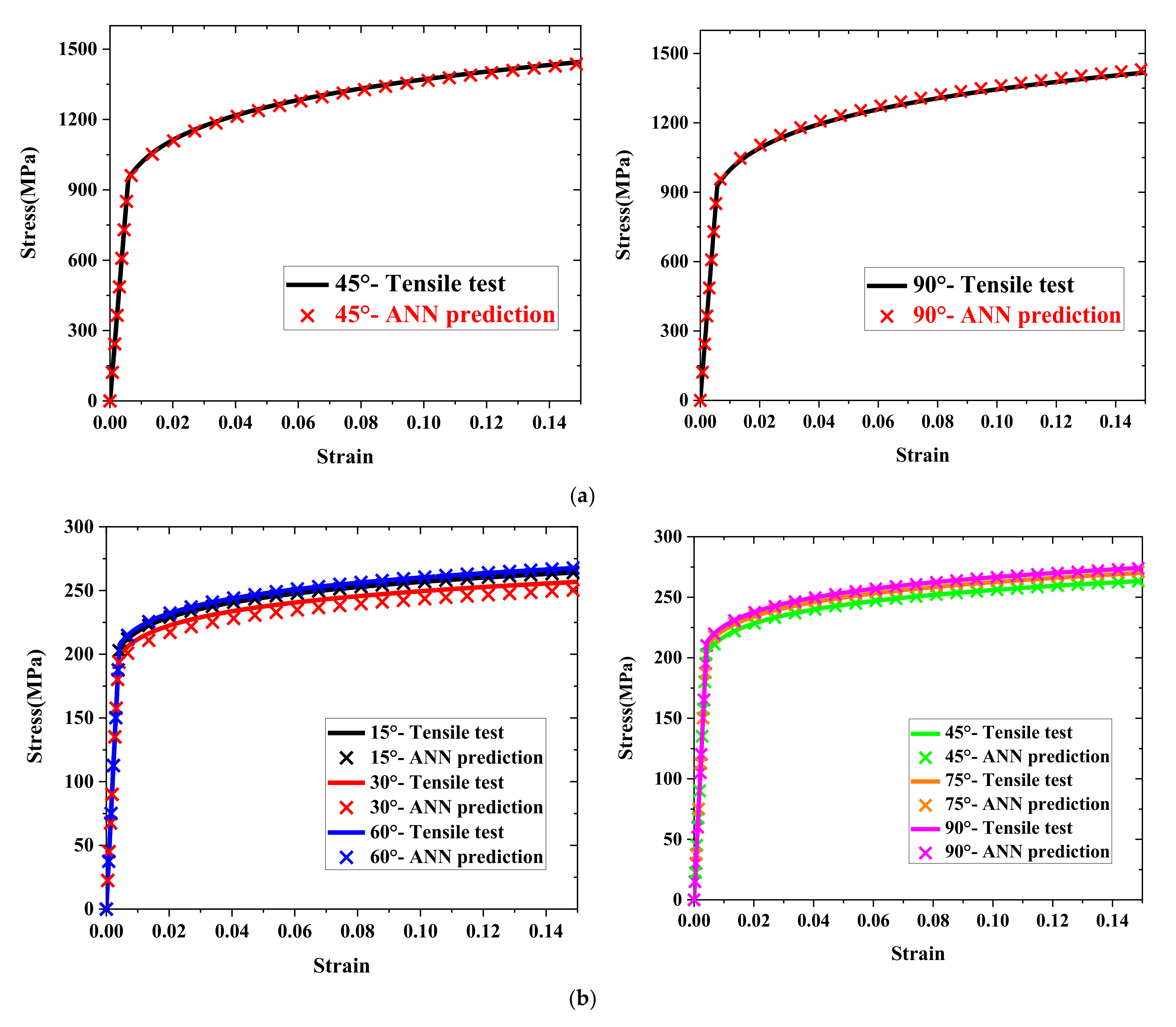
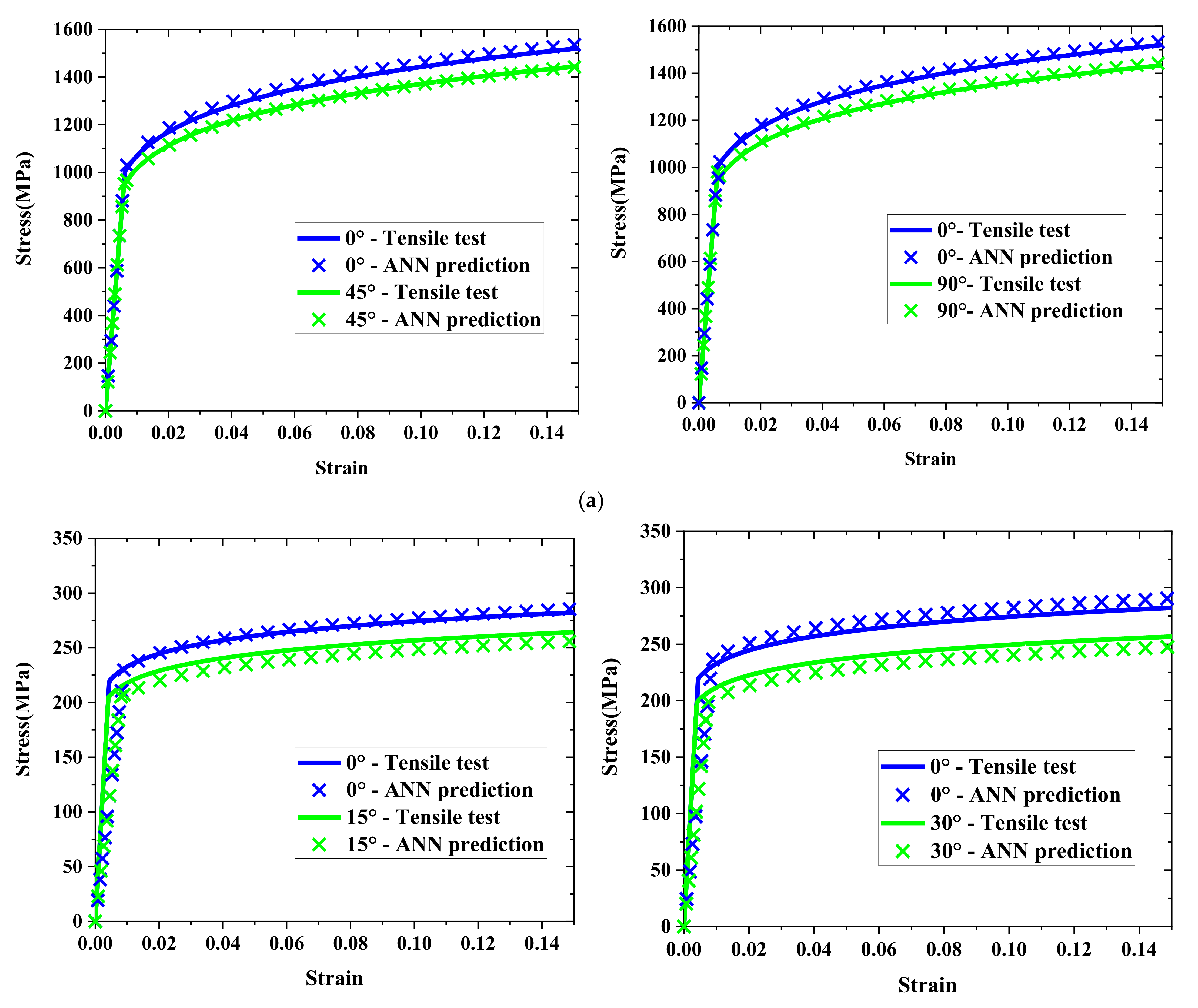
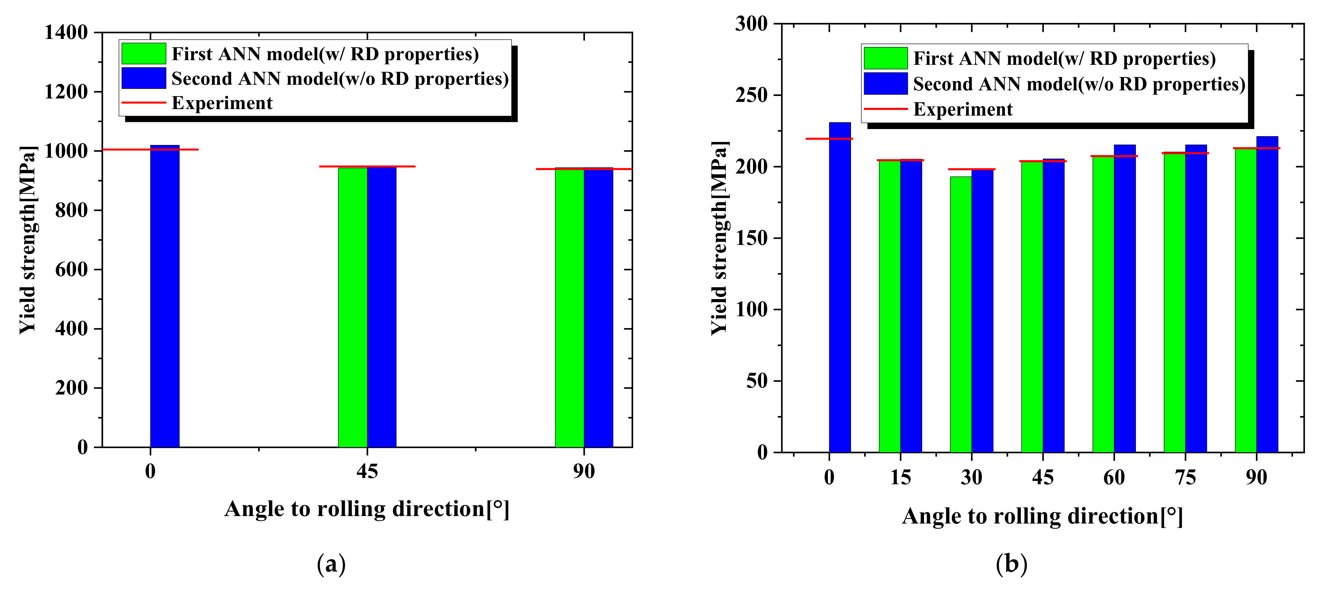
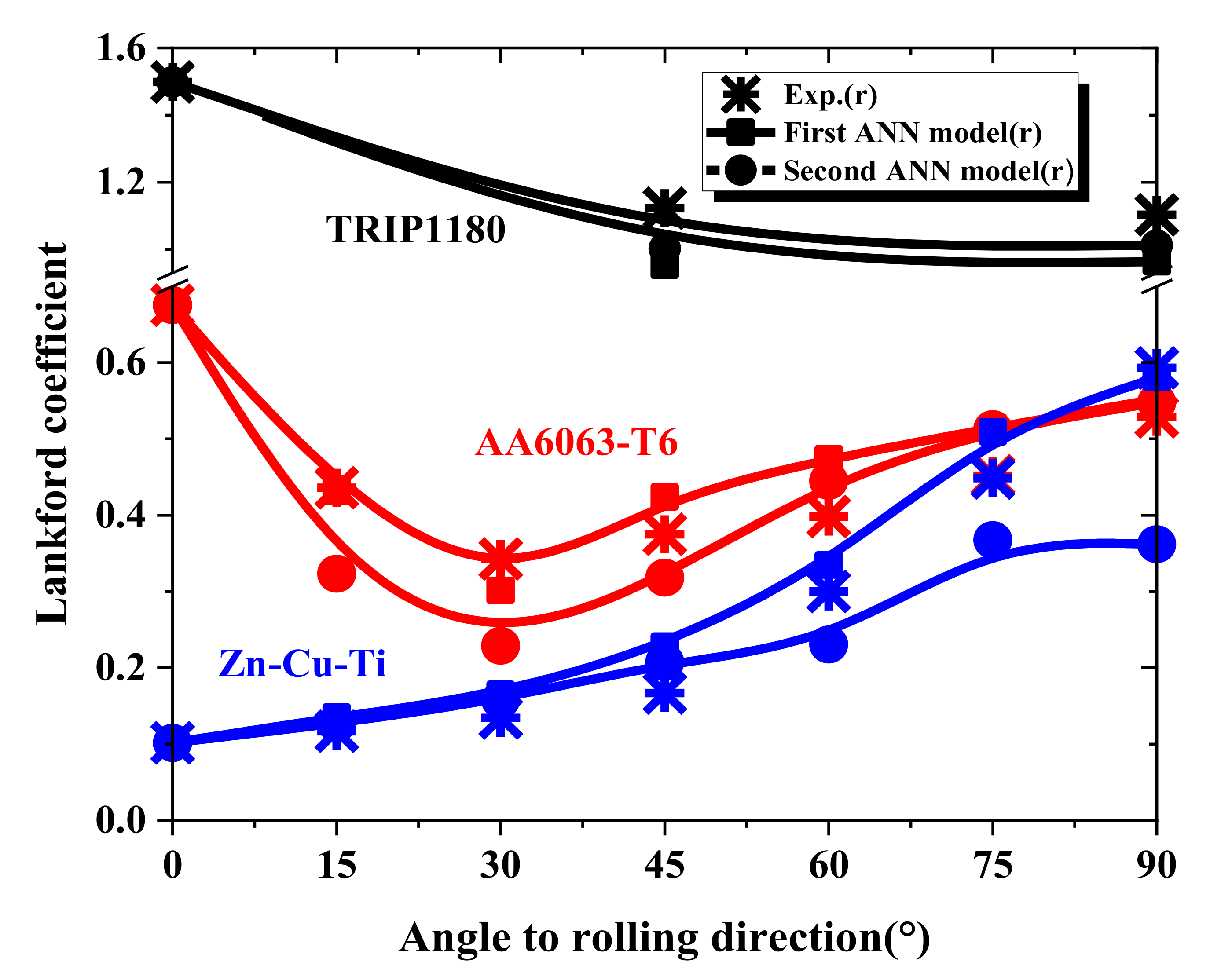
- The proposed two types of artificial neural network models can predict the anisotropic properties of materials, where the first prediction model, with RD characteristics as input parameters, can predict the yield strength ratio and the Lankford coefficient well. On the other hand, in cases without RD characteristics as input parameters, the second model provides a comprehensive prediction of the material’s properties, including its elastic–plastic and anisotropic properties.
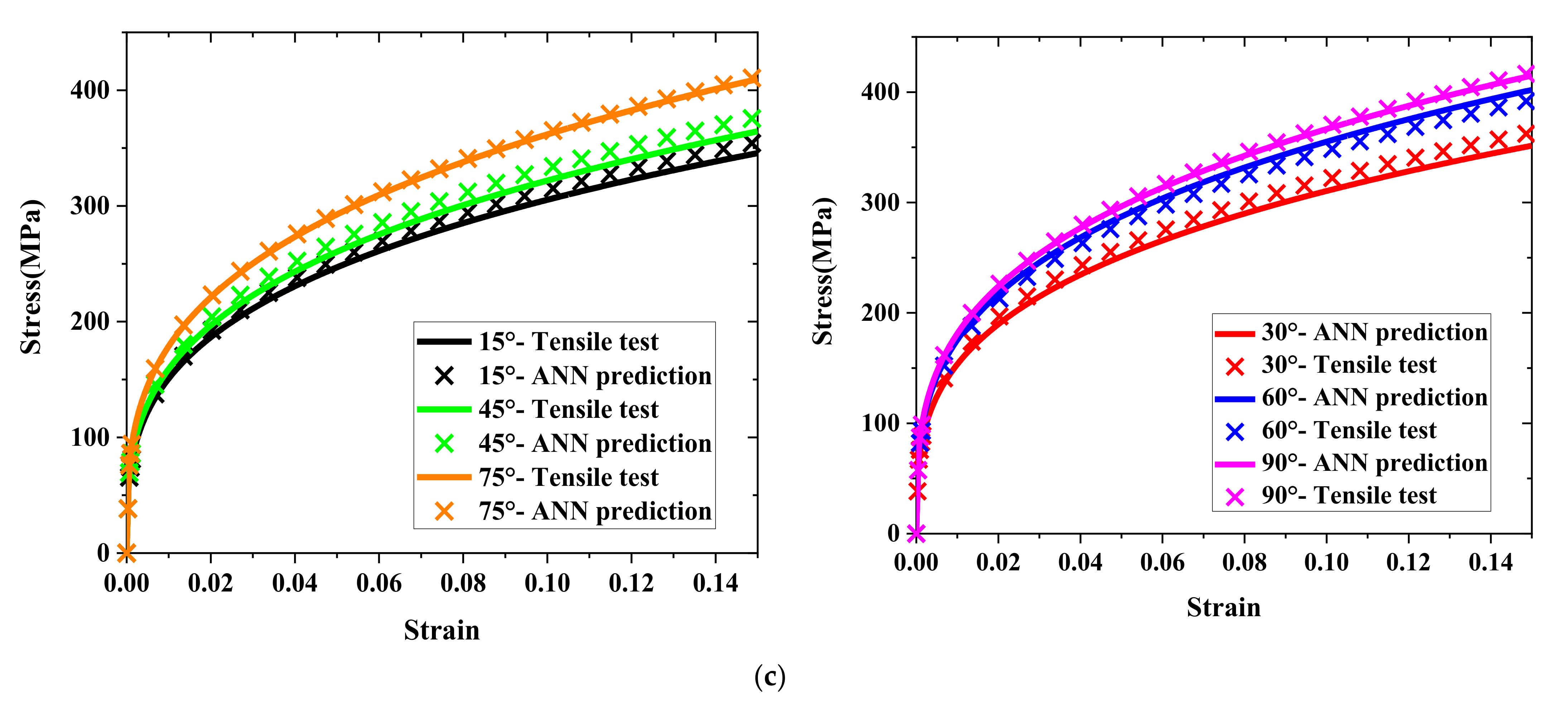
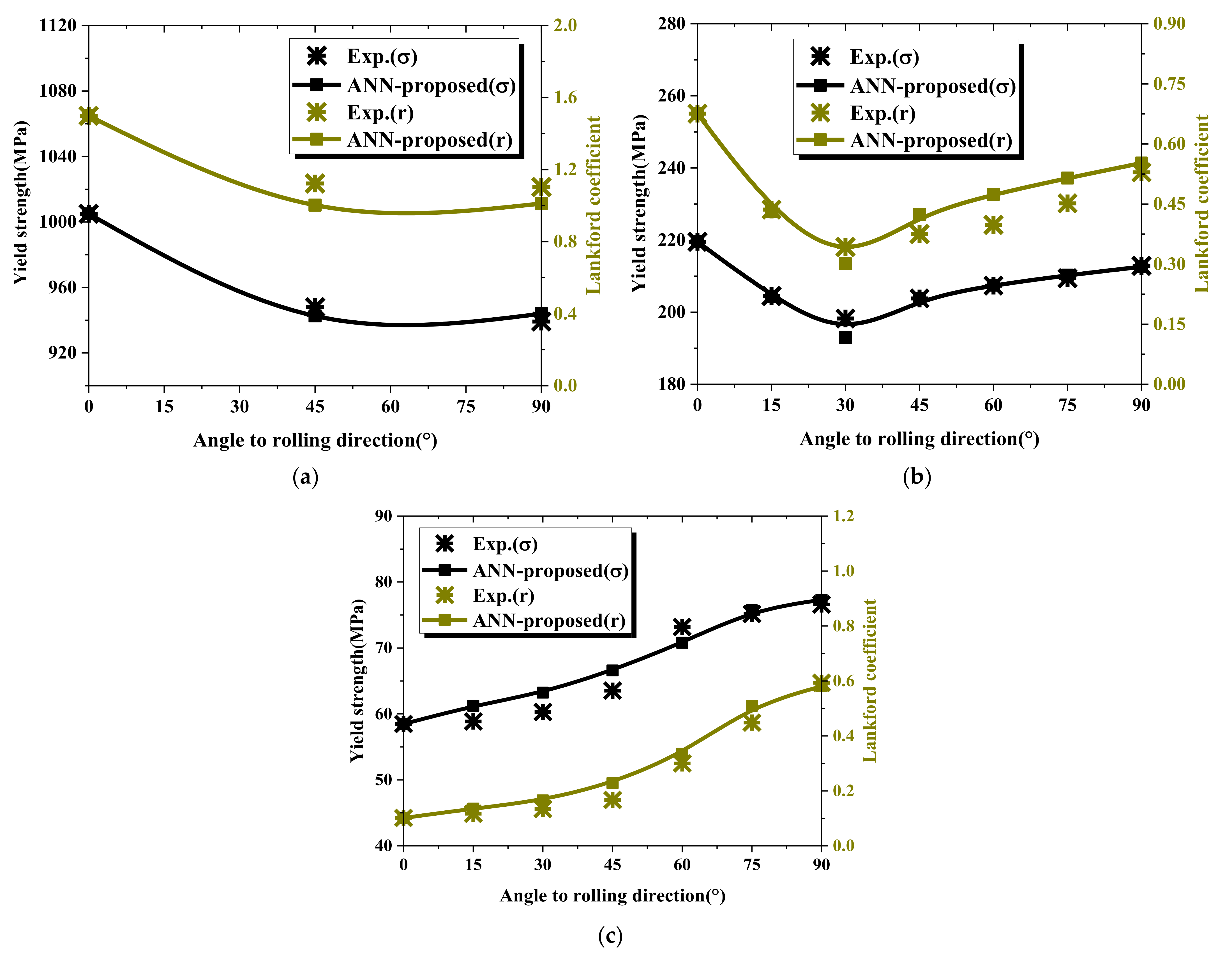
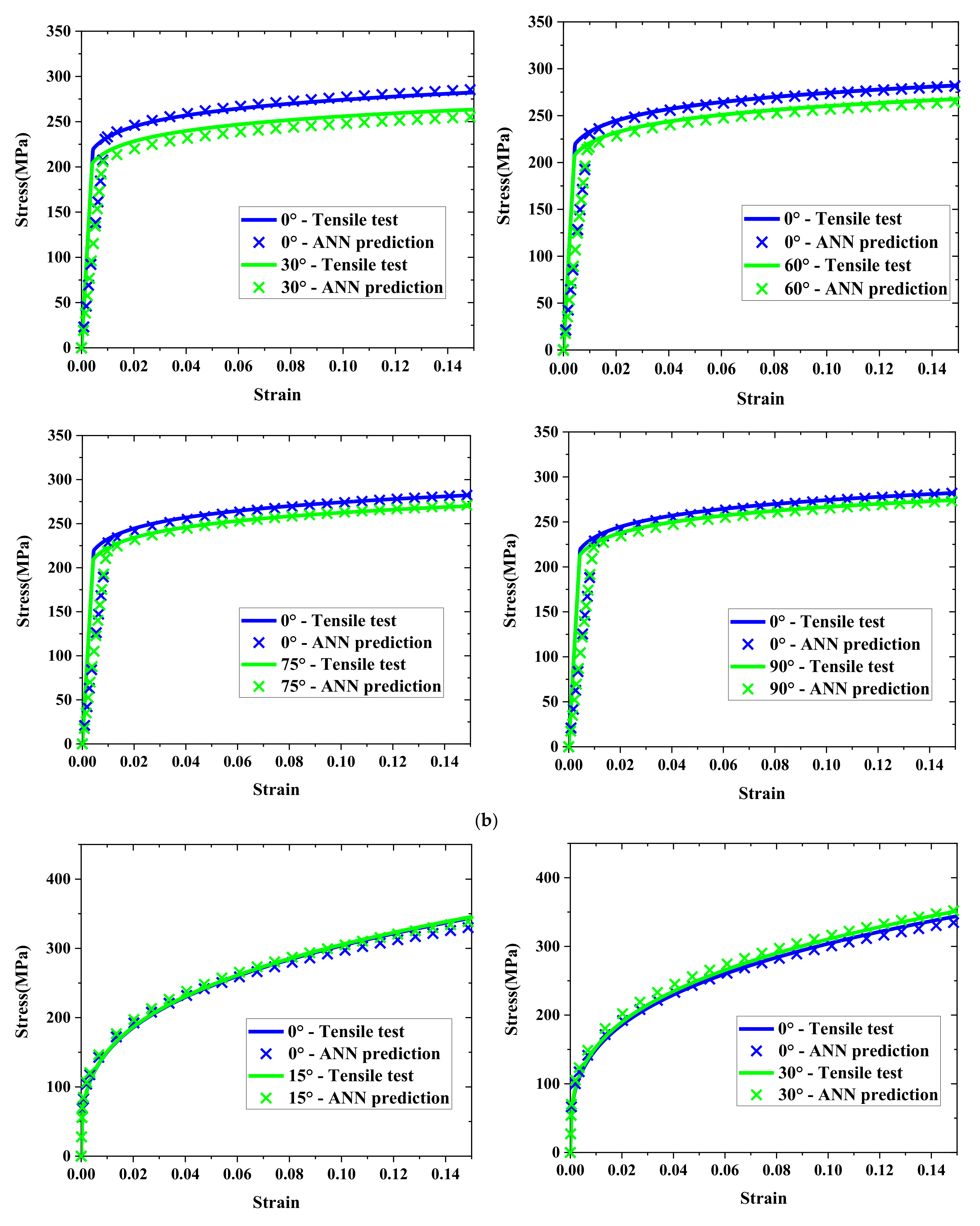
- The predicted yield strength ratios using the first model of TRIP1180, AA6063-T6, and Zn-Cu-Ti alloy had a maximum deviation from the experimental results of 0.6%, 2.6%, and 4.9%, respectively. At the same time, the Lankford coefficient predicted by our model was consistent with the experimental results. The deviations in the predicted stress–strain flow curves were all less than 5%. Furthermore, the flow curve predicted for each material using the improved ANN model showed a maximum deviation from the tensile test of 4.7%.
- In future work, the deeper prediction ANN model for the anisotropy of Young’s modulus and hardness exponent can be constructed to comprehensively predict the anisotropy properties of materials with larger Young’s modulus and hardness exponent. Furthermore, it is possible to improve the ANN model, which can predict the anisotropy properties by utilizing the Chaboche model after undergoing the complex stress state.
Author Contributions
Funding
Institutional Review Board Statement
Informed Consent Statement
Data Availability Statement
Conflicts of Interest
References
- Yoon, J.H.; Cazacu, O.; Yoon, J.W.; Dick, R.E. Earing predictions for strongly textured aluminum sheets. Int. J. Mech. Sci. 2010, 52, 1563–1578. [Google Scholar] [CrossRef]
- Khalfallah, A.; Alves, J.L.; Oliveira, M.C.; Menezes, L.F. Influence of the characteristics of the experimental data set used to identify anisotropy parameters. Simul. Model. Pract. Theory 2015, 53, 15–44. [Google Scholar] [CrossRef] [Green Version]
- Singh, A.; Basak, S.; Prakash, L.P.S.; Roy, G.G.; Jha, M.N.; Mascarenhas, M.; Panda, S.K. Prediction of earing defect and deep drawing behavior of commercially pure titanium sheets using CPB06 anisotropy yield theory. J. Manuf. Process. 2018, 33, 256–267. [Google Scholar] [CrossRef]
- Aldalur, E.; Suárez, A.; Veiga, F. Metal transfer modes for Wire Arc Additive Manufacturing Al-Mg alloys: Influence of heat input in microstructure and porosity. J. Mater. Process. Technol. 2021, 297, 117271. [Google Scholar] [CrossRef]
- Oliver, W.C.; Pharr, G.M. Measurement of hardness and elastic modulus by instrumented indentation: Advances in understanding and refinements to methodology. J. Mater. Res. 2014, 19, 3–20. [Google Scholar] [CrossRef]
- Jeong, K.J.; Lee, H.J.; Kwon, O.M.; Jung, J.W.; Kwon, D.I.; Ha, H.N. Prediction of uniaxial tensile flow using finite element-based indentation and optimized artificial neural networks. Mater. Des. 2020, 196, 109104. [Google Scholar] [CrossRef]
- Field, J.; Swain, M. A simple predictive model for spherical indentation. J. Mater. Res. 1993, 8, 297–306. [Google Scholar] [CrossRef]
- Peng, G.J.; Xu, F.L.; Chen, J.F.; Wang, H.D.; Hu, J.J.; Zhang, T.H. Evaluation of Non-Equibiaxial Residual Stresses in Metallic Materials via Instrumented Spherical Indentation. Metals 2020, 10, 440. [Google Scholar] [CrossRef] [Green Version]
- Jang, J.I. Estimation of residual stress by instrumented indentation: A review. J. Ceram. Process. Res. 2009, 10, 391–400. [Google Scholar]
- Shen, L.; He, Y.; Liu, D.; Gong, Q.; Zhang, B.; Lei, J. A novel method for determining surface residual stress components and their directions in spherical indentation. J. Mater. Res. 2015, 30, 1078–1089. [Google Scholar] [CrossRef]
- Nakamura, T.; Gu, Y. Identification of elastic–plastic anisotropic parameters using instrumented indentation and inverse analysis. Mech. Mater. 2007, 39, 340–356. [Google Scholar] [CrossRef]
- Yoneda, K.; Yonezu, A.; Hirakata, H.; Minoshima, K. Estimations of anisotropic plastic properties of engineering steel from spherical impressions. Int. J. Appl. Mech. 2010, 2, 355–379. [Google Scholar] [CrossRef]
- Yonezu, A.; Yoneda, K.; Hirakata, H.; Sakihara, M.; Minoshima, K. A simple method to evaluate anisotropic plastic properties based on dimensionless function of single spherical indentation—Application to SiC whisker-reinforced aluminum alloy. Mater. Sci. Eng. A 2010, 527, 7646–7657. [Google Scholar] [CrossRef]
- Wang, M.Z.; Wu, J.J.; Zhan, X.P.; Guo, R.C.; Hui, Y.; Fan, H. On the determination of the anisotropic plasticity of metal materials by using instrumented indentation. Mater. Des. 2016, 111, 98–107. [Google Scholar] [CrossRef]
- Wu, J.J.; Wang, M.Z.; Hui, Y.; Zhang, Z.K.; Fan, H. Identification of anisotropic plasticity properties of materials using spherical indentation imprint mapping. Mater. Sci. Eng. A 2018, 723, 269–278. [Google Scholar] [CrossRef]
- Huber, N.; Konstantinidis, A.; Tsakmakis, C.H. Determination of Poisson’s Ratio by Spherical Indentation Using Neural Networks—Part I: Theory. J. Appl. Mech. 2004, 68, 218–223. [Google Scholar] [CrossRef]
- Tho, K.K.; Swaddiwudhipong, S.; Liu, Z.S.; Hua, J. Artificial neural network model for material characterization by indentation. Model. Simul. Mater. Sci. Eng. 2004, 12, 1055–1062. [Google Scholar] [CrossRef]
- Muliana, A.; Steward, R.; Haj-Ali, R.M.; Saxena, A. Artificial Neural Network and Finite Element Modeling of Nanoindentation Tests. Metall. Mater. Trans. A 2002, 33, 1939–1947. [Google Scholar] [CrossRef]
- Mahmoudi, A.H.; Nourbakhsh, S.H. A Neural Networks approach to characterize material properties using the spherical indentation test. Procedia Eng. 2001, 10, 3062–3067. [Google Scholar] [CrossRef] [Green Version]
- Lu, L.; Dao, M.; Kumarc, P.; Ramamurtyc, U.; Karniadakisa, G.E.; Sureshd, S. Extraction of mechanical properties of materials through deep learning from instrumented indentation. Proc. Natl. Acad. Sci. USA 2020, 117, 7052–7062. [Google Scholar] [CrossRef] [Green Version]
- Dao, M.; Chollacoop, N.; Van Vliet, K.J.; Venkatesh, T.A.; Suresh, S. Computational modeling of the forward and reverse problems in instrumented sharp indentation. Acta Mater. 2001, 49, 3899–3918. [Google Scholar] [CrossRef] [Green Version]
- Lee, H.; Lee, J.H.; Pharr, G.M. A numerical approach to spherical indentation techniques for material property evaluation. J. Mech. Phys. Solids 2005, 53, 2037–2069. [Google Scholar] [CrossRef]
- Taljat, B.; Pharr, G.M. Development of pile-up during spherical indentation of elastic–plastic solids. Int. J. Solids Struct. 2004, 41, 3891–3904. [Google Scholar] [CrossRef]
- Hill, R. A theory of the yielding and plastic flow of anisotropic metals. Math. Phys. Sci. 1948, 193, 281–297. [Google Scholar]
- ABAQUS. Analysis User’s Manual Version 6.9; Software for Finite Element Analysis and Computer-Aided Engineering; ABAQUS Inc.: Providence, RI, USA, 2009. [Google Scholar]
- Wang, M.; Wu, J.; Wu, H.; Zhang, Z.; Fan, H. A novel approach to estimate the plastic anisotropy of metallic materials using cross-sectional indentation-application to extruded magnesium alloy AZ31B. Materials 2017, 10, 1065. [Google Scholar] [CrossRef] [Green Version]
- Doerner, M.F.; Nix, W.D. A method for interpreting the data from depth-sensing indentation instruments. J. Mater. Res. 1986, 1, 601–609. [Google Scholar] [CrossRef]
- Karthik, V.; Visweswaran, P.; Bhushan, A.; Pawaskar, D.N.; Kasiviswanathan, K.V.; Jayakumar, T.; Raj, B. Finite element analysis of spherical indentation to study pile-up/sink-in phenomena in steels and experimental validation. Int. J. Mech. Sci. 2012, 54, 74–83. [Google Scholar] [CrossRef]
- Crawford, G.A.; Chawla, N.; Koopman, M.; Carlisle, K.; Chawla, K.K. Effect of Mounting Material Compliance on Nanoindentation Response of Metallic Materials. Adv. Eng. Mater. 2009, 11, 45–51. [Google Scholar] [CrossRef]
- Kurlov, A.S.; Gusev, A.I. Tungsten Carbides: Structure, Properties and Application in Hardmetals; Springer International Publishing: Berlin/Heidelberg, Germany, 2013. [Google Scholar]
- Zíta, D.; Hanus, P.; Schmidová, E.; Zajíc, J. Determining of the machine compliance using instrumented indentation test and finite element method. Mater. Sci. Eng. 2019, 461, 012095. [Google Scholar] [CrossRef]


| Young’s Modulus (MPa) | Yield Strength (MPa) | Strain Hardening Exponent (n) | Lankford Coefficient (r) | ||
|---|---|---|---|---|---|
| TRIP1180 | 0° | 161,994 | 1005 | 0.13 | 1.499 |
| 45° | 948 | 1.123 | |||
| 90° | 939 | 1.103 | |||
| AA6063-T6 | 0° | 50,000 | 219 | 0.0712 | 0.675 |
| 15° | 204 | 0.436 | |||
| 30° | 198 | 0.343 | |||
| 45° | 203 | 0.375 | |||
| 60° | 207 | 0.398 | |||
| 75° | 209 | 0.452 | |||
| 90° | 212 | 0.529 | |||
| Zn-Cu-Ti alloy | 0° | 127,700 | 58 | 0.306 | 0.101 |
| 15° | 59 | 0.117 | |||
| 30° | 60 | 0.134 | |||
| 45° | 63 | 0.167 | |||
| 60° | 73 | 0.300 | |||
| 75° | 75 | 0.449 | |||
| 90° | 76 | 0.593 |
| Direction | TRIP1180 | AA6063-T6 | Zn-Cu-Ti Alloy | |
|---|---|---|---|---|
| Indentation height () | 0° | 52.315 | 58.747 | 76.597 |
| 15° | − | 63.026 | 74.496 | |
| 30° | − | 65.357 | 72.689 | |
| 45° | 53.521 | 63.161 | 70.363 | |
| 60° | − | 60.717 | 68.673 | |
| 75° | − | 59.539 | 65.604 | |
| 90° | 53.587 | 59.109 | 65.520 | |
| Indentation length () | 0° | 158.385 | 160.625 | 191.154 |
| 15° | − | 170.201 | 190.768 | |
| 30° | − | 175.103 | 187.953 | |
| 45° | 159.306 | 170.885 | 184.407 | |
| 60° | − | 165.869 | 178.858 | |
| 75° | − | 162.791 | 178.190 | |
| 90° | 160.481 | 162.335 | 177.520 |
| Indenter | Material | |
|---|---|---|
| E (MPa) | 700,000 | 161,994 |
| v | 0.31 | 0.31 |
| Load–Depth Curve | Residual Indentation Mark | Properties of the RD Stress–Strain Curve (Only Works on the First Model) |
|---|---|---|
|
|
|
| Properties | Range |
|---|---|
| Young’s modulus (E) | 5~210 GPa |
| Yield strength () | 30~3000 MPa |
| Hardness exponent (n) | 0~0.5 |
| Yield strength ratio (m) | 0.1~2 |
| First Model | Yield Strength Ratio (m) | |||
|---|---|---|---|---|
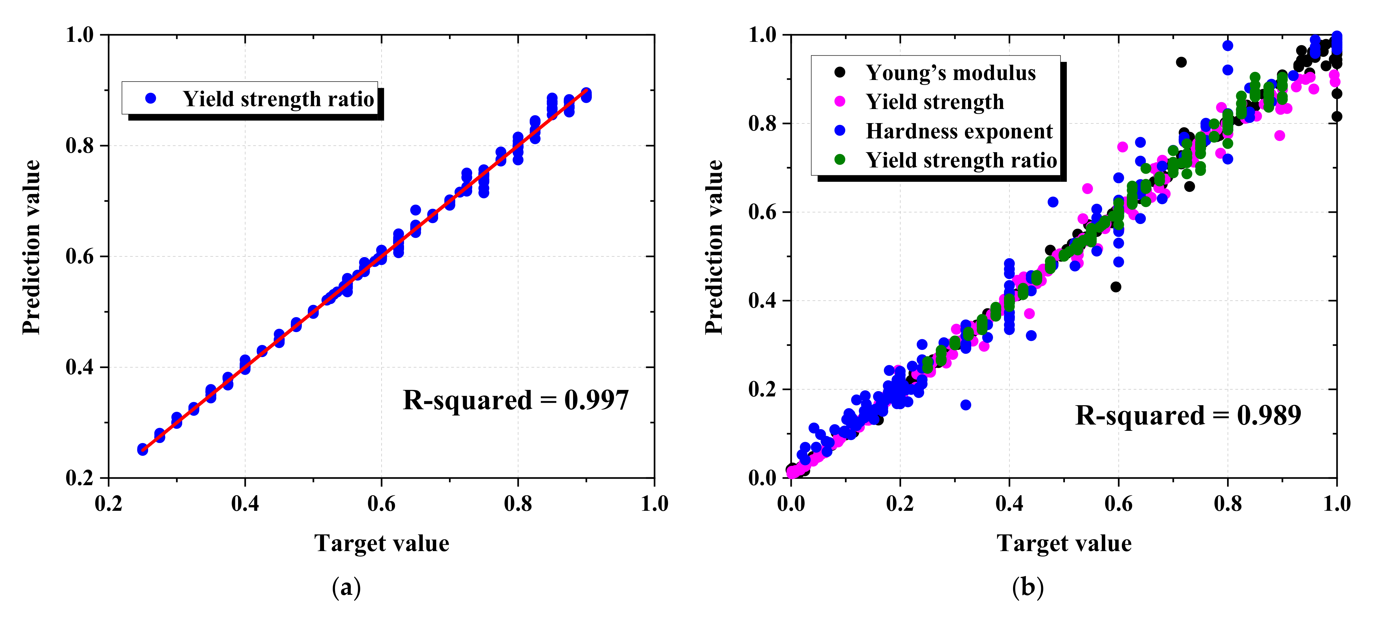
| Correlation (R-squared) | 99.764% | |||
| Loss (MAE) | 0.285% | |||
| Second model | Young’s modulus (E) | Yield strength () | Hardness exponent (n) | Yield strength ratio(m) |
| Correlation (R-squared) | 99.004% | 99.079% | 98.231% | 99.400% |
| Loss (MAE) | 1.161% | 1.509% | 2.506% | 0.913% |
| Direction | Yield Strength | ||||
|---|---|---|---|---|---|
| Tensile Test Result (MPa) | ANN Prediction Result (MPa) | Deviation | Deviation in the Flow Curve Area | ||
| TRIP1180 | 45° | 948.023 | 942.603 | 0.572% | 0.499% |
| 90° | 939.164 | 944.000 | 0.515% | 0.433% | |
| AA6063-T6 | 15° | 204.497 | 204.404 | 0.042% | 0.042% |
| 30° | 198.227 | 192.956 | 2.578% | 2.445% | |
| 45° | 203.815 | 203.807 | 0.004% | 0.003% | |
| 60° | 207.376 | 207.478 | 0.050% | 0.045% | |
| 75° | 209.392 | 210.239 | 0.408% | 0.372% | |
| 90° | 212.856 | 212.612 | 0.117% | 0.105% | |
| Zn-Cu-Ti alloy | 15° | 58.859 | 61.238 | 4.042% | 2.787% |
| 30° | 60.291 | 63.221 | 4.860% | 3.347% | |
| 45° | 63.528 | 66.586 | 4.814% | 3.331% | |
| 60° | 73.177 | 70.79 | 3.262% | 2.274% | |
| 75° | 75.169 | 75.707 | 0.716% | 0.496% | |
| 90° | 76.602 | 77.306 | 0.919% | 0.637% | |
| Material | Properties | Direction | Tensile Test Result | ANN Prediction Result |
|---|---|---|---|---|
| TRIP1180 | Young’s modulus (E) | 0°–45° | 161,994 | 163,075 |
| 0°–90° | 161,994 | 163,266 | ||
| Yield strength () | 0°–45° | 1005/948.023 | 1019.760/948.614 | |
| 0°–90° | 1005/939.164 | 1012.740/943.840 | ||
| Hardness exponent (n) | 0°–45° | 0.130 | 0.129 | |
| 0°–90° | 0.130 | 0.130 | ||
| Yield strength ratio (m) | 0°–45° | 1.060 | 1.075 | |
| 0°–90° | 1.070 | 1.073 | ||
| Deviation of the flow curve area | 0°–45° | 1.172%/0.045% | ||
| 0°–90° | 0.924%/0.695% | |||
| AA6063-T6 | Young’s modulus (E) | 0°–15° | 50,000 | 25,509 |
| 0°–30° | 50,000 | 27,065 | ||
| 0°–45° | 50,000 | 25,587 | ||
| 0°–60° | 50,000 | 23,739 | ||
| 0°–75° | 50,000 | 23,354 | ||
| 0°–90° | 50,000 | 23,193 | ||
| Yield strength () | 0°–15° | 219.520 /204.497 | 230.893 /205.238 | |
| 0°–30° | 219.520 /198.227 | 235.867 /198.374 | ||
| 0°–45° | 219.520 /203.815 | 231.663 /205.375 | ||
| 0°–60° | 219.520 /207.376 | 230.116 /215.263 | ||
| 0°–75° | 219.520 /209.392 | 227.903 /218.089 | ||
| 0°–90° | 219.520 /212.856 | 228.652 /221.134 | ||
| Hardness exponent (n) | 0°–15° | 0.0712 | 0.0755 | |
| 0°–30° | 0.0712 | 0.0733 | ||
| 0°–45° | 0.0712 | 0.0744 | ||
| 0°–60° | 0.0712 | 0.0735 | ||
| 0°–75° | 0.0712 | 0.0784 | ||
| 0°–90° | 0.0712 | 0.077 | ||
| Yield strength ratio (m) | 0°–15° | 1.073469 | 1.125 | |
| 0°–30° | 1.107423 | 1.189 | ||
| 0°–45° | 1.077061 | 1.128 | ||
| 0°–60° | 1.058566 | 1.069 | ||
| 0°–75° | 1.048374 | 1.045 | ||
| 0°–90° | 1.031311 | 1.034 | ||
| Deviation of the flow curve area | 0°–15° | 0.483%/4.504% | ||
| 0°–30° | 1.604%/4.629% | |||
| 0°–45° | 0.388%/4.361% | |||
| 0°–60° | 1.848%/2.667% | |||
| 0°–75° | 1.930%/1.622% | |||
| 0°–90° | 2.027%/2.214% | |||
| Zn-Cu-Ti alloy | Young’s modulus (E) | 0°–15° | 127,700 | 185,697 |
| 0°–30° | 127,700 | 180,248 | ||
| 0°–45° | 127,700 | 170,498 | ||
| 0°–60° | 127,700 | 167,321 | ||
| 0°–75° | 127,700 | 138,878 | ||
| 0°–90° | 127,700 | 138,642 | ||
| Yield strength () | 0°–15° | 58.477 /58.859 | 63.538 /65.843 | |
| 0°–30° | 58.477 /60.291 | 61.618 /66.114 | ||
| 0°–45° | 58.477 /63.528 | 59.194 /66.361 | ||
| 0°–60° | 58.477 /73.177 | 58.143 /66.298 | ||
| 0°–75° | 58.477 /75.169 | 54.336 /66.752 | ||
| 0°–90° | 58.477 /76.602 | 54.514 /66.807 | ||
| Hardness exponent (n) | 0°–15° | 0.306 | 0.271 | |
| 0°–30° | 0.306 | 0.278 | ||
| 0°–45° | 0.306 | 0.288 | ||
| 0°–60° | 0.306 | 0.297 | ||
| 0°–75° | 0.306 | 0.311 | ||
| 0°–90° | 0.306 | 0.311 | ||
| Yield strength ratio (m) | 0°–15° | 0.993 | 0.965 | |
| 0°–30° | 0.969 | 0.932 | ||
| 0°–45° | 0.920 | 0.892 | ||
| 0°–60° | 0.799 | 0.877 | ||
| 0°–75° | 0.778 | 0.814 | ||
| 0°–90° | 0.763 | 0.816 | ||
| Deviation of the flow curve area | 0°–15° | 1.244%/0.867% | ||
| 0°–30° | 0.417%/2.576% | |||
| 0°–45° | 0.326%/2.760% | |||
| 0°–60° | 3.284%/3.049% | |||
| 0°–75° | 0.120%/3.285% | |||
| 0°–90° | 0.013%/4.597% | |||
Publisher’s Note: MDPI stays neutral with regard to jurisdictional claims in published maps and institutional affiliations. |
© 2022 by the authors. Licensee MDPI, Basel, Switzerland. This article is an open access article distributed under the terms and conditions of the Creative Commons Attribution (CC BY) license (https://creativecommons.org/licenses/by/4.0/).
Share and Cite
Xia, J.; Won, C.; Kim, H.; Lee, W.; Yoon, J. Artificial Neural Networks for Predicting Plastic Anisotropy of Sheet Metals Based on Indentation Test. Materials 2022, 15, 1714. https://doi.org/10.3390/ma15051714
Xia J, Won C, Kim H, Lee W, Yoon J. Artificial Neural Networks for Predicting Plastic Anisotropy of Sheet Metals Based on Indentation Test. Materials. 2022; 15(5):1714. https://doi.org/10.3390/ma15051714
Chicago/Turabian StyleXia, Jiaping, Chanhee Won, Hyunggyu Kim, Wonjoo Lee, and Jonghun Yoon. 2022. "Artificial Neural Networks for Predicting Plastic Anisotropy of Sheet Metals Based on Indentation Test" Materials 15, no. 5: 1714. https://doi.org/10.3390/ma15051714
APA StyleXia, J., Won, C., Kim, H., Lee, W., & Yoon, J. (2022). Artificial Neural Networks for Predicting Plastic Anisotropy of Sheet Metals Based on Indentation Test. Materials, 15(5), 1714. https://doi.org/10.3390/ma15051714