
Numerical Simulation of Dry Ice Compaction Process: Comparison of the Mohr–Coulomb Model with the Experimental Results


Abstract
1. Introduction
- -
- -
- -
2. Materials and Methods
2.1. Materials
2.1.1. Dry Ice Snow
2.1.2. Compression
2.1.3. Elastoplastic Properties of Dry Ice as a Function of Density
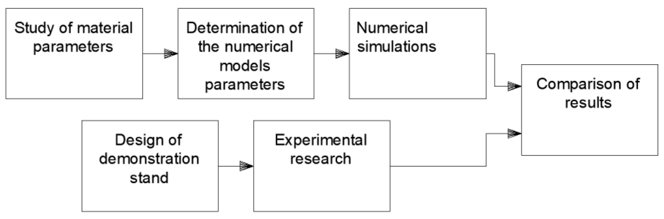
2.2. Method and Numerical Model
3. Results and Discussion
- -
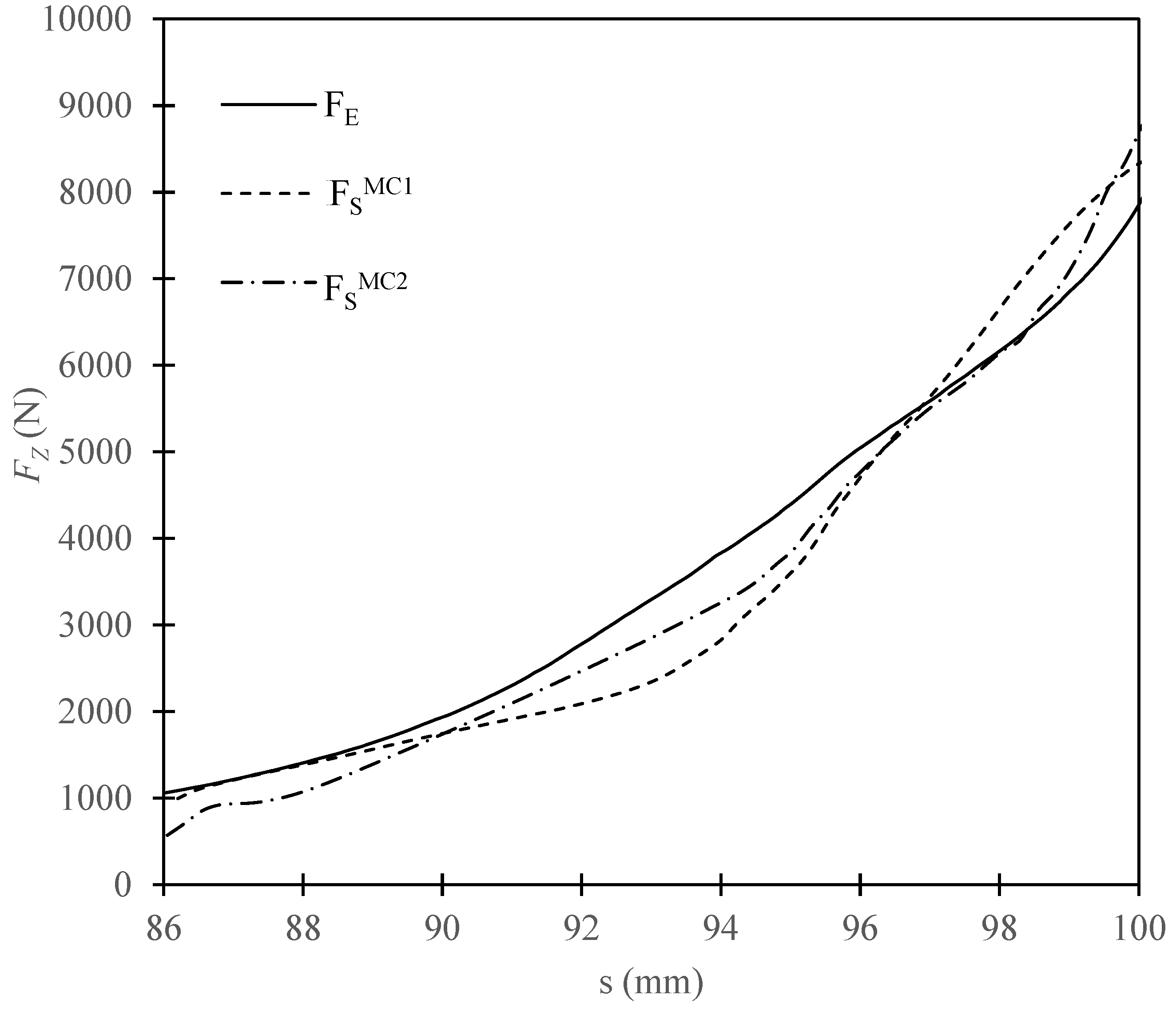
- the Mohr–Coulomb model using constant input parameters gives an accurate prediction of the maximum force acting during compression of dry ice,
- -
- variable input parameters, depending on the value of PEEQ would, however, be more appropriate if it is required to determine the change of the applied force during the compression process.
4. Conclusions
Author Contributions
Funding
Institutional Review Board Statement
Informed Consent Statement
Data Availability Statement
Conflicts of Interest
References
- Piotrowska, K.; Kruszelnicka, W.; Bałdowska-Witos, P.; Kasner, R.; Rudnicki, J.; Tomporowski, A.; Flitzikowski, J.; Opielak, M. Assessmet of the environmental impact of a car tire throughout its life cycle using the Ica method. Materials 2019, 12, 4177. [Google Scholar] [CrossRef] [PubMed]
- Wilczyński, D.; Berdychowski, M.; Wojtkowiak, D.; Górecki, J.; Wałęsa, K. Experimental and numerical tests of the compaction process of loose material in the form of sawdust. MATEC Web Conf. 2019, 254, 02042. [Google Scholar] [CrossRef]
- Gierz, Ł.; Warguła, Ł.; Kukla, M.; Koszela, K.; Zawiachel, T.S. Computer aided modeling of wood chips transport by means of a belt conveyor with use of discrete element method. Appl. Sci. 2020, 10, 9091. [Google Scholar] [CrossRef]
- Uhryński, A.; Bembenek, M. The thermographic analysis of the agglomeration process in the roller press of pillow-shaped briquettes. Materials 2022, 15, 2870. [Google Scholar] [CrossRef] [PubMed]
- Wilczyński, D.; Berdychowski, M.; Talaśka, K.; Wojtkowiak, D. Experimental and numerical analysis of the effect of compaction conditions on briquette properties. Fuel 2021, 288, 119613. [Google Scholar] [CrossRef]
- Wojtkowiak, D.; Talaśka, K.; Wilczyński, D.; Górecki, J.; Wałęsa, K. Determinig the power consumption of the atomatic device for belt perforation based on the dynamic model. Energies 2021, 14, 317. [Google Scholar] [CrossRef]
- Tan, Z.; Songtao, L.; Hong, Z.; Yanjiang, C. Elastoplastic integration method of mohr coulomb criterion. Geotechnics 2022, 2, 599–614. [Google Scholar] [CrossRef]
- Cassiani, G.; Brovelli, A.; Hueckel, T. A strain-rate-dependent modified Cam-Clay model for the simulation of soil/rock compaction. Géoméch. Energy Environ. 2017, 11, 42–51. [Google Scholar] [CrossRef]
- Berdychowski, M.; Górecki, J.; Biszczanik, A.; Wałęsa, K. Numerical simulation of dry ice compaction process: Comparison of drucker-prager/cap and cam clay models with experimental results. Materials 2022, 15, 5771. [Google Scholar] [CrossRef]
- Górecki, J.; Talaśka, K.; Wałęsa, K.; Wilczyński, D.; Wojtkowiak, D. Mathematical model describing the influence of geometrical parameters of multichannel dies on the limit force of dry ice extrusion process. Materials 2020, 13, 3317. [Google Scholar] [CrossRef]
- Mikołajczak, A.; Krawczyk, P.; Kurkus-Gruszecka, M.; Badyda, K. Analysis of the Liquid Natural Gas Energy Storage basing on the mathematical model. Energy Procedia 2019, 159, 231–236. [Google Scholar] [CrossRef]
- Dzido, A.; Krawczyk, P.; Kurkus-Gruszecka, M. Numerical analysis of dry ice blasting convergent-divergent supersonic nozzle. Energies 2019, 12, 4787. [Google Scholar] [CrossRef]
- Liu, Y.; Calvert, G.; Hare, C.; Ghadiri, M.; Matsusaka, S. Size measurement of dry ice particles produced from liquid carbon dioxide. J. Aerosol Sci. 2012, 48, 1–9. [Google Scholar] [CrossRef]
- Liu, Y.; Hirama, D.; Matusaka, S. Particle removal process during application of impinging dry ice jet. Powder Technol. 2017, 217, 607–613. [Google Scholar] [CrossRef]
- Górecki, J.; Malujda, I.; Talaka, K.; Wojtkowiak, D. Dry ice compaction in piston extrusion process. Acta Mech. Autom. 2017, 11, 313–316. [Google Scholar] [CrossRef][Green Version]
- Dzido, A.; Krawczyk, P.; Badyda, K.; Chondrokostas, P. Impact of operating parameters on the performance of dry-ice blasting nozzle. Energy 2021, 214, 118847. [Google Scholar] [CrossRef]
- Górecki, J. Development of a testing station for empirical verification of the algebraic model of dry ice piston extrusion. Acta Mech. Autom. 2021, 15, 107–112. [Google Scholar] [CrossRef]
- Talaśka, K. Study of Research and Modeling of the Compaction Processes of Loose and Disintegrated Materials; Politechnika Poznańska: Poznań, Poland, 2018. (In Polish) [Google Scholar]
- Biszczanik, A.; Wałęsa, K.; Kukla, M.; Górecki, J. The influence of density on the value of young’s modulus for dry ice. Materials 2021, 14, 7763. [Google Scholar] [CrossRef]
- Biszczanik, A.; Górecki, J.; Kukla, M.; Wałęsa, K.; Wojtkowiak, D. Experimental investigation on the effect of dry ice compression on the poisson ratio. Materials 2022, 15, 1555. [Google Scholar] [CrossRef]
- Diarra, H.; Mazel, V.; Boillon, A.; Rehault, L.; Busignies, V.; Bureau, S.; Tchoreloff, P. Finite Element Method (FEM) modeling of the powder compaction of cosmetic products: Comparison between simulated and experimental results. Powder Technol. 2012, 224, 233–240. [Google Scholar] [CrossRef]
- Brewin, P.; Coube, O.; Doremus, P.; Tweed, J. Modeling of Powder Die Compaction; Springer: London, UK, 2008. [Google Scholar]
- Han, L.; Elliott, J.; Bentham, A.; Mills, A.; Amidon, G.; Hancock, B. A modified Drucker-Prager Cap model for die compaction simulation of pharmaceutical powders. Int. J. Solids Struct. 2008, 45, 3088–3106. [Google Scholar] [CrossRef]
- Berdychowski, M.; Talaśka, K.; Malujda, I.; Kukla, M. Application og the Mohr-Columb model for simulation the biomass compaction proces. IOP Conf. Ser. Mater. Sci. Eng. 2020, 776, 012066. [Google Scholar] [CrossRef]
- Abaqus Documentation; Dassault Systemes: Paris, France, 2017.
- Greaves, G.; Greer, A.; Lakes, R.; Rouxel, T. Poissons’s ratio and modern materials. Nat. Mater. 2011, 10, 823–837. [Google Scholar] [CrossRef] [PubMed]
- Kaufmann, E.; Attree, N.; Bradwell, T.; Hagermann, A. Hardness and yield strength of co2 ice under martian temperature conditions. J. Geophys. Res. Planets 2020, 125, e2019JE006217. [Google Scholar] [CrossRef]
- Górecki, J.; Malujda, I.; Talaśka, K.; Tarkowski, P.; Kukla, M. Influence of the value of limit densification stress on the quality of the pellets during the agglomeration process of CO2. Procedia Eng. 2016, 136, 2190–2195. [Google Scholar] [CrossRef]
- Górecki, J.; Fierek, A.; Wilczyński, D.; Wałęsa, K. The influence of the limit stress value on the sublimation rate during the dry ice densification process. IOP Conf. Series Mater. Sci. Eng. 2020, 776, 012072. [Google Scholar] [CrossRef]
- Devroye, L.; Schäfer, D.; Györfi, L.; Walk, H. The estimation problem of minimum mean squared error. Stat. Decis. 2009, 21, 15–28. [Google Scholar] [CrossRef]
- Bilal, M.; Masud, S.; Athar, S. FPGA design for statistics-inspired approximate sum-of-squared-error computation in multimedia applications. IEEE Trans. Circuits Syst. II Express Briefs 2012, 59, 8. [Google Scholar] [CrossRef]


| Cohesion Yield Stress | Abs Plastic Deformation | Friction Angle | Dilation Angle |
|---|---|---|---|
| 500,000 | 0 | 15 | 0 |
| 600,000 | 0.4 | ||
| 700,000 | 0.8 | ||
| 1,000,000 | 1 |
| Young’s Modulus | Poisson’s Ratio | PEEQ |
|---|---|---|
| 36,590,000 | 0.02 | 0–0.5 |
| 45,142,000 | 0.05 | 0.5–0.9 |
| 60,900,000 | 0.07 | 0.9–1.5 |
| 152,100,000 | 0.4 | 1.5–2 |
| 823,820,000 | 0.46 | 2–5 |
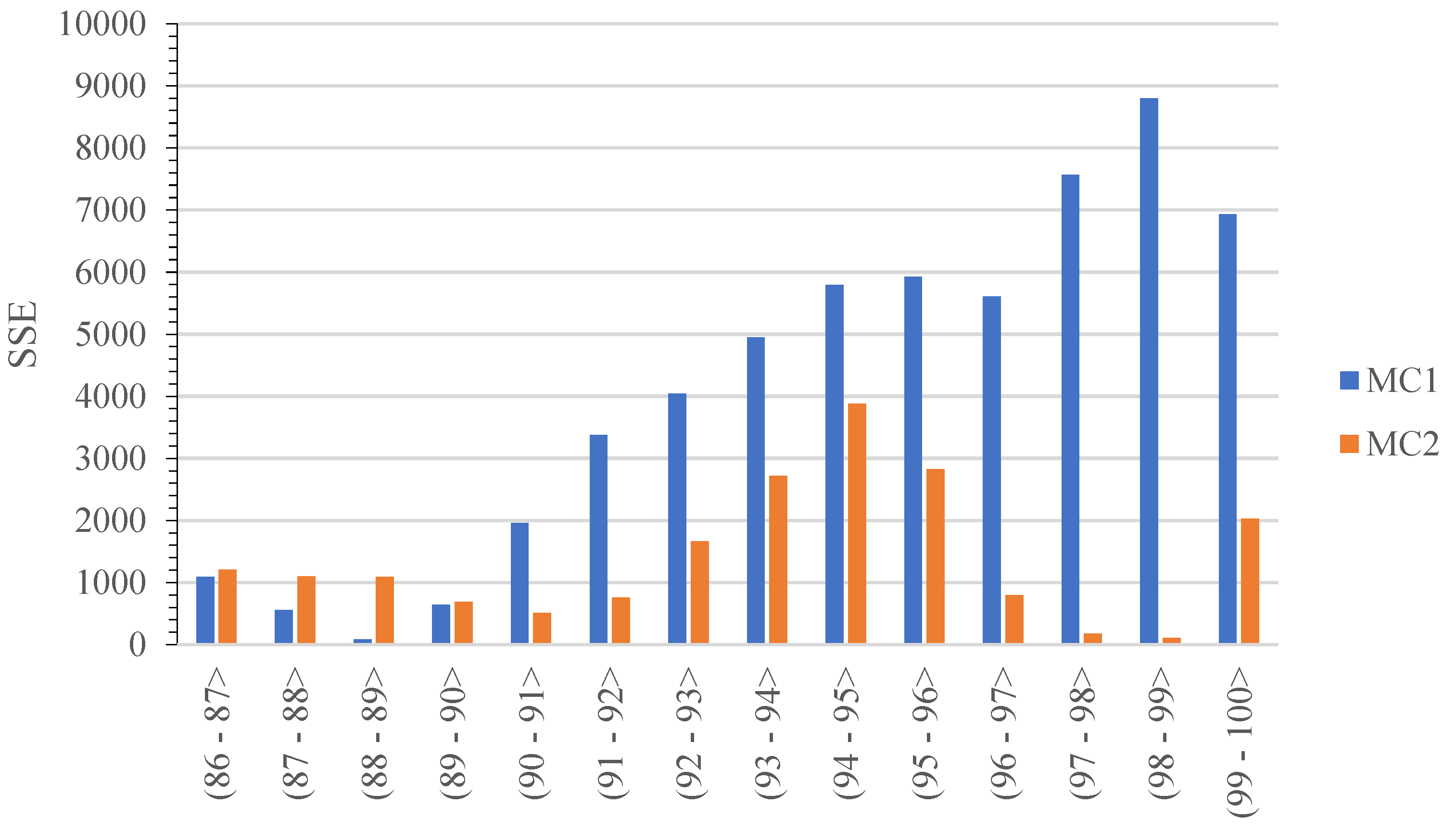
| Range of s, mm | SSEMC1 | SSEMC2 |
|---|---|---|
| (86–87 | 1.1 × 10⁶ | 1.2 × 10⁶ |
| (87–88 | 5.6 × 10⁵ | 1.1 × 10⁶ |
| (88–89 | 8.2 × 10⁴ | 1.1 × 10⁶ |
| (89–90 | 6.4 × 10⁵ | 6.9 × 10⁵ |
| (90–91 | 2.0 × 10⁶ | 5.1 × 10⁵ |
| (91–92 | 3.4 × 10⁶ | 7.6 × 10⁵ |
| (92–93 | 4.0 × 10⁶ | 1.7 × 10⁶ |
| (93–94 | 5.0 × 10⁶ | 2.7 × 10⁶ |
| (94–95 | 5.8 × 10⁶ | 3.9 × 10⁶ |
| (95–96 | 5.9 × 10⁶ | 2.8 × 10⁶ |
| (96–97 | 5.6 × 10⁶ | 8.0 × 10⁵ |
| (97–98 | 7.6 × 10⁶ | 1.8 × 10⁵ |
| (98–99 | 8.8 × 10⁶ | 1.1 × 10⁵ |
| (99–100 | 6.9 × 10⁶ | 2.0 × 10⁶ |
| (86–100 | 5.7 × 10⁷ | 2.0 × 10⁷ |
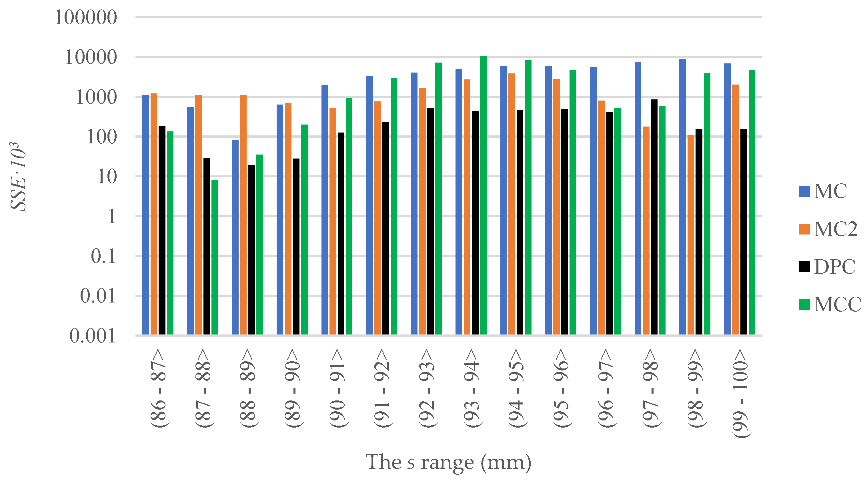
| Range of s, mm | SSEMC1 | SSEMC2 | SSEDPC | SSECC |
|---|---|---|---|---|
| 1.1 × 10⁶ | 1.2 × 10⁶ | 1.34 × 10⁵ | 1.81 × 10⁵ | |
| 5.6 × 10⁵ | 1.1 × 10⁶ | 8 × 10³ | 2.9 × 10⁴ | |
| 8.2 × 10⁴ | 1.1 × 10⁶ | 3.5 × 10⁴ | 1.9 × 10⁴ | |
| 6.4 × 10⁵ | 6.9 × 10⁵ | 2.01 × 10⁵ | 2.8 × 10⁴ | |
| 2.0 × 10⁶ | 5.1 × 10⁵ | 9.21 × 10⁵ | 1.27 × 10⁵ | |
| 3.4 × 10⁶ | 7.6 × 10⁵ | 3.027 × 10⁶ | 2.38 × 10⁵ | |
| 4.0 × 10⁶ | 1.7 × 10⁶ | 7.268 × 10⁶ | 5.16 × 10⁵ | |
| 5.0 × 10⁶ | 2.7 × 10⁶ | 1.0334 × 10⁷ | 4.42 × 10⁵ | |
| 5.8 × 10⁶ | 3.9 × 10⁶ | 8.474 × 10⁶ | 4.56 × 10⁵ | |
| 5.9 × 10⁶ | 2.8 × 10⁶ | 4.660 × 10⁶ | 4.85 × 10⁵ | |
| 5.6 × 10⁶ | 8.0 × 10⁵ | 5.31 × 10⁵ | 4.07 × 10⁵ | |
| 7.6 × 10⁶ | 1.8 × 10⁵ | 5.73 × 10⁵ | 8.5 × 10⁵ | |
| 8.8 × 10⁶ | 1.1 × 10⁵ | 3.962 × 10⁶ | 1.53 × 10⁵ | |
| 6.9 × 10⁶ | 2.0 × 10⁶ | 4.705 × 10⁶ | 1.54 × 10⁵ | |
| (86–100 | 5.7 × 10⁷ | 2.0 × 10⁷ | 4.09 × 10⁶ | 4.48 × 10⁷ |
| κ (%) | ||
|---|---|---|
| 8.397 | 6.37 | |
| 8.340 | 5.65 | |
| 8.064 | 2.15 | |
| 8.328 | 5.50 | |
| 7.894 |
Publisher’s Note: MDPI stays neutral with regard to jurisdictional claims in published maps and institutional affiliations. |
© 2022 by the authors. Licensee MDPI, Basel, Switzerland. This article is an open access article distributed under the terms and conditions of the Creative Commons Attribution (CC BY) license (https://creativecommons.org/licenses/by/4.0/).
Share and Cite
Berdychowski, M.; Górecki, J.; Wałęsa, K. Numerical Simulation of Dry Ice Compaction Process: Comparison of the Mohr–Coulomb Model with the Experimental Results. Materials 2022, 15, 7932. https://doi.org/10.3390/ma15227932
Berdychowski M, Górecki J, Wałęsa K. Numerical Simulation of Dry Ice Compaction Process: Comparison of the Mohr–Coulomb Model with the Experimental Results. Materials. 2022; 15(22):7932. https://doi.org/10.3390/ma15227932
Chicago/Turabian StyleBerdychowski, Maciej, Jan Górecki, and Krzysztof Wałęsa. 2022. "Numerical Simulation of Dry Ice Compaction Process: Comparison of the Mohr–Coulomb Model with the Experimental Results" Materials 15, no. 22: 7932. https://doi.org/10.3390/ma15227932
APA StyleBerdychowski, M., Górecki, J., & Wałęsa, K. (2022). Numerical Simulation of Dry Ice Compaction Process: Comparison of the Mohr–Coulomb Model with the Experimental Results. Materials, 15(22), 7932. https://doi.org/10.3390/ma15227932