Article

Semi-Infinite Structure Analysis with Bimodular Materials with Infinite Element

1
School of Traffic and Transportation Engineering, Changsha University of Science and Technology, Changsha 410114, China
2
Institute of Construction and Architecture, Slovak Academy of Sciences, 84503 Bratislava, Slovakia
3
School of Engineering and Materials Science, Queen Mary University of London, London E1 4NS, UK
*
Author to whom correspondence should be addressed.
Materials 2022, 15(2), 641; https://doi.org/10.3390/ma15020641
Submission received: 27 November 2021 / Revised: 11 January 2022 / Accepted: 13 January 2022 / Published: 15 January 2022

Abstract

:
The modulus of elasticity of some materials changes under tensile and compressive states is simulated by constructing a typical material nonlinearity in a numerical analysis in this paper. The meshless Finite Block Method (FBM) has been developed to deal with 3D semi-infinite structures in the bimodular materials in this paper. The Lagrange polynomial interpolation is utilized to construct the meshless shape function with the mapping technique to transform the irregular finite domain or semi-infinite physical solids into a normalized domain. A shear modulus strategy is developed to present the nonlinear characteristics of bimodular material. In order to verify the efficiency and accuracy of FBM, the numerical results are compared with both analytical and numerical solutions provided by Finite Element Method (FEM) in four examples.

1. Introduction

It has been shown that certain materials such as composites, porous materials, rocks, cement concrete and asphalt concrete, etc., show significant differences in their strength in tension and compression states. The modulus of elasticity as well as the Poisson’s ratio of the material may also change under tensile and compressive states [1,2,3]. Take the concrete material as an example; the compressive modulus is about 1.5~2 times the tensile modulus [4,5,6]. So, for an accurate numerical simulation, this characteristic of material has to be considered. It constructs a typical material nonlinear model.
In order to evaluate bearing capacity and stability, the civil structure with the soil–foundation interaction is commonly investigated numerically, including airport runways, highway pavement, stacking dock, mineral deposit, geotechnical slope and so on. The soil medium is simplified as an infinite or semi-infinite domain. The most common approach with FEM is to use massive elements to simulate an unbounded domain. The application of large-scale finite element discretization could result in an increase in computational burden [7]. Furthermore, the inaccurate results could be obtained due to the truncated boundaries in the numerical procedure. To overcome this difficulty, the Boundary Integral Equations Method (BIEM), also known as the Boundary Element Method (BEM), is coupled with the FEM [8,9]. However, it is difficult to derive the fundamental solutions in general cases, especially for non-homogeneous and nonlinearity of materials. Meanwhile, the semi-analytical finite element method was developed to reduce the time cost of 3D model simulation [10,11] and applied in pavement structural analysis [12,13], but it mainly focuses on linear analysis or problems without complicated loads. The unbounded problems can be overcome by introducing mapped infinite elements, i.e., utilizing the infinite element to extend the FEM to unbounded domain problems [14,15,16,17]. The shape function describes the far-field characteristic of the problem, which can be obtained using mapping to transform the global infinite region into a local finite domain by Bettess et al. [17,18,19,20]. As an alternative, these issues can be solved with the meshless methods coupling with an infinite-mapping technique [7].
In engineering analysis, the linear elasticity of material is not valid for general issue. The material mechanical properties are closely related to their micro structure. The scanning images of the building materials are shown in Figure 1 and present similar mottled patterns at different scales. The heterogeneity is manifested in the micro-scale for the metal materials, and its mechanical properties accord with the linear elastic hypothesis. For the rock or concrete materials, their heterogeneity is displayed in the mesoscale and the assumption of linear elasticity sometimes produces computational errors which cannot be ignored.
Commercial numerical software in engineering, including ABAQUS, are widely used in engineering and manufacturing. However, it is still a challenging task to solve bimodular problems efficiently [21,22,23,24,25,26]. Nevertheless, the development of new numerical methods is always attractive to solve difficult and complicated engineering problems. Unlike the traditional numerical method, the computational framework of the meshless method was based on the scattered nodes. In the 1990s, the meshless method was developed based upon the Galerkin method. In 1992, the diffuse element method (DEM) was proposed by Nayroles et al. [27]. The Moving-Least Square (MLS) method was introduced to construct the meshless shape functions with Galerkin method in numerical discretization. In 1994, Belytschkoet al. presented the Element-Free Galerkin method (EFGM) [28], in which Lagrange was employed to ensure the boundary conditions were being satisfied. Since then, the EFGM has been widely used to simulate the fracture failure of materials and to show its superiority over the traditional FEM [29,30]. In 1996, Belytschko et al. published a comprehensive review [31] which attracted exclusive attention in computational mechanics. This can be regarded as the beginning of the meshless method in numerical engineering. Another important development was the introduction of the local weak form methods. In 1998, Atluri et al. proposed the Meshless Local Petrov-Galerkin (MLPG) method [32]. The discrete system equation is based on a nodal assembly with more conciseness in numerical implementation. In 1995, Liu et al. proposed a Reproducing Kernel Particle Method (RKPM) approximation [33,34,35]. Thereafter, several meshless methods were developed such as the Method of Fundamental Solution (MFS) [36,37,38], the local Radial Point Interpolation Method (RPIM) [39,40,41], the local Radial Basis Function (RBF) collocation method [42,43,44] and the Meshless Intervention-Point (MIP) method [45], etc. In 2014, Wen et al. proposed the meshless FBM [46]. In the finite block method, the mapping technique is implemented numerically with the infinite elements for the infinite domain problems [7]. Afterwards, the FBM is successfully applied to nonlinear elasticity problems, contact problems and heat conduction problems [47,48,49]. It has been demonstrated in the analysis of bimodular problems for two-dimensional problems [50].
In this paper, the FBM is extended to three-dimensional semi-infinite structures in bimodular materials. The infinite block mapping technique is introduced to present the semi-infinite structure and implemented with the meshless finite block method to construct the intrinsic constitutive equations in iterative analysis. The meshless finite block method with the infinite block mapping technique is formulated for 3D bimodular problems. The FEM solution is considered as a benchmark for numerical analysis, and the accuracy of the proposed method is observed by ABAQUS with subroutine UMAT developed for bimodular materials.

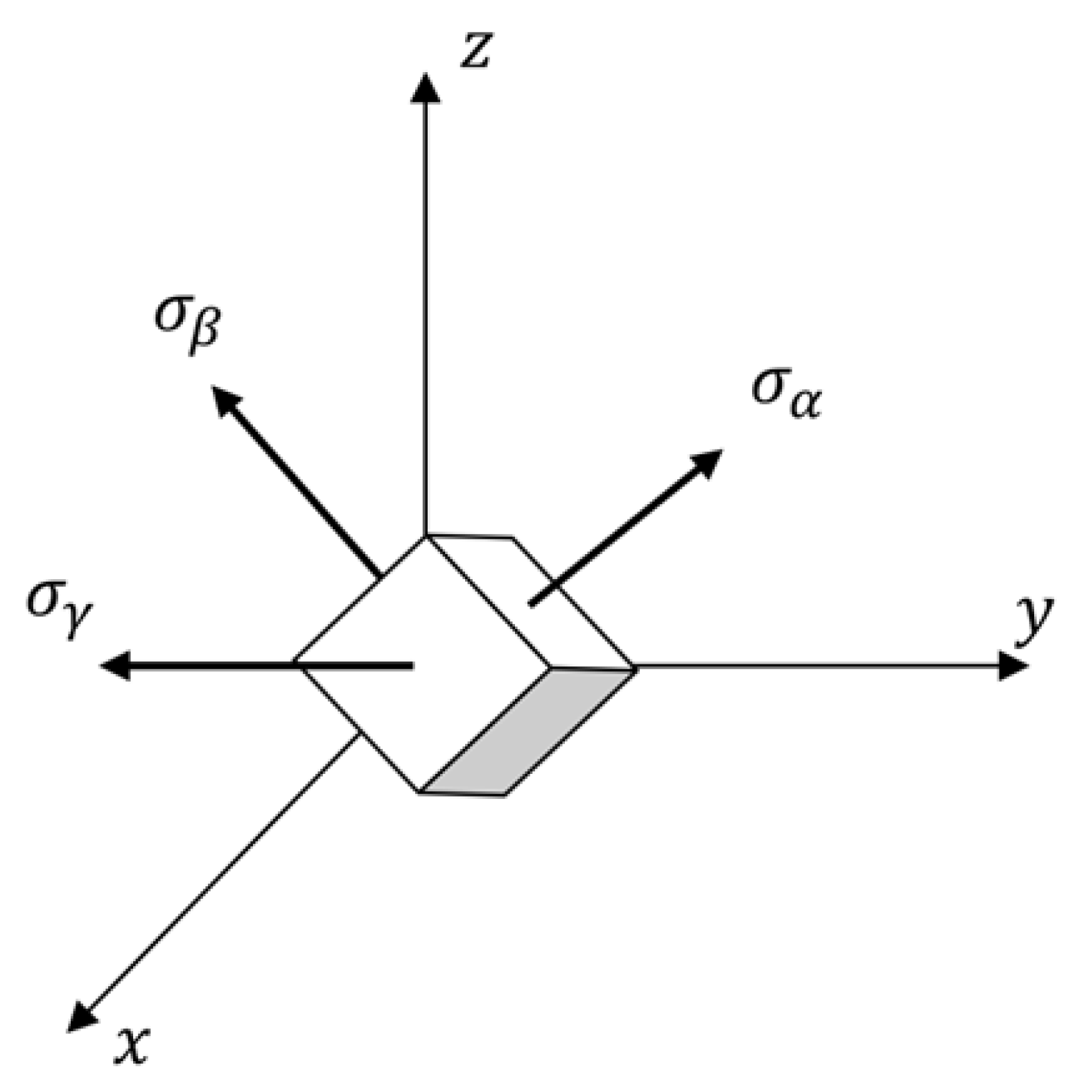
2. Bimodular Material Constitutive Equations

Suppose σ α , σ β and σ γ are principal stresses, as shown in Figure 2. The generalized Hooke’s law, in matrix form, as
ε ˜ = A σ ˜   or   σ ˜ = Q I ε ˜
where A is the flexibility matrix, QI is the elasticity matrix, ε ˜ is the nodal strain vector in the principal directions and σ ˜ is the nodal stress vector in the principal directions, which are defined as
A = ( a 11 a 12 a 13 0 0 0 a 21 a 22 a 23 0 0 0 a 31 a 32 a 33 0 0 0 0 0 0 a 44 0 0 0 0 0 0 a 55 0 0 0 0 0 0 a 66 ) , Q I = A 1
ε ˜ = { ε α , ε β , ε γ , ε β γ , ε α γ , ε α β } T
σ ˜ = { σ α , σ β , σ γ , σ β γ , σ α γ , σ α β } T
With the analytical theory proposed by Ambartsumyan and complemented with shear moduli [1,21,22], it is assumed that a i j = v / E = v + / E + , a j j = 1 / E + or 1 / E , (I = 1, j = 1, 2, 3), where E + and E present as the tensile and compressive moduli respectively, v + and v are the tensile and compressive Poisson’s ratio, respectively; a 44 = 1 / G β γ , a 55 = 1 / G α γ , a 66 = 1 / G α β , in which, G β γ , G α γ and G α β are the shear moduli. The shear stresses or strains in the principal directions are zero. According to the shear moduli algorithm [13], it is assumed that the axes x, y and z tend to axes α , β and γ , respectively. Then, we have
G β γ = l i m l 1 , m 2 , n 3 1 l 2 , l 3 , m 1 , m 3 , n 1 n 2 0 G y z = l i m l 1 , m 2 , n 3 1 l 2 , l 3 , m 1 , m 3 , n 1 n 2 0 τ y z γ y z G α γ = l i m l 1 , m 2 , n 3 1 l 2 , l 3 , m 1 , m 3 , n 1 n 2 0 G x z = l i m l 1 , m 2 , n 3 1 l 2 , l 3 , m 1 , m 3 , n 1 n 2 0 τ x z γ x z G α β = l i m l 1 , m 2 , n 3 1 l 2 , l 3 , m 1 , m 3 , n 1 n 2 0 G x y = l i m l 1 , m 2 , n 3 1 l 2 , l 3 , m 1 , m 3 , n 1 n 2 0 τ x y γ x y
There are three cases to obtain G β γ , G α γ and G α β ,
(1)
If all three principal stresses are equal, i.e., σ α = σ β = σ γ , we have
a.
If σ α 0 , then
G β γ = G α γ = G α β = G = E 2 ( 1 + v )
b.
If σ α > 0 , then
G β γ = G α γ = G α β = G + = E + 2 ( 1 + v + )
(2)
If only two of the three principal stresses are equal, i.e., σ α = σ β σ γ , we hold
G α β = σ α σ γ 2 ( ε α ε γ ) = G α γ = G β γ
(3)
If all three principal stresses are not equal, i.e., σ α σ β σ γ , we have
G β γ = σ β σ γ 2 ( ε β ε γ ) , G α γ = σ α σ γ 2 ( ε α ε γ )   and   G α β = σ α σ β 2 ( ε α ε β )
In the Cartesian coordinate system, the directional cosines for each principal strain are defined as
α = ( l 1 , l 2 , l 3 ) β = ( m 1 , m 2 , m 3 ) γ = ( n 1 , n 2 , n 3 )
The strain vector in different coordinate systems is obtained, in matrix form, as
ε ˜ = L ε ,
where ε is the strain vector in Cartesian’s coordinate system and L is the transformation matrix defined by
L = ( l 1 2 m 1 2 n 1 2 m 1 n 1 l 1 n 1 l 1 m 1 l 2 2 m 2 2 n 2 2 m 2 n 2 l 2 n 2 l 2 m 2 l 3 2 m 3 2 n 3 2 m 3 n 3 l 3 n 3 l 3 m 3 2 l 2 l 3 2 m 2 m 3 2 n 2 n 3 m 2 n 3 + m 3 n 2 l 2 n 3 + l 3 n 2 l 2 m 3 + l 3 m 2 2 l 1 l 3 2 m 1 m 3 2 n 1 n 3 m 1 n 3 + m 3 n 1 l 1 n 3 + l 3 n 1 l 1 m 3 + l 3 m 1 2 l 1 l 2 2 m 1 m 2 2 n 1 n 2 m 1 n 2 + m 2 n 1 l 1 n 2 + l 2 n 1 l 1 m 2 + l 2 m 1 )
The strain energy density U in terms of the principal strains and elastic matrix, at each node, yields
U = 1 2 ε ˜ T Q I ε ˜ = 1 2 ε T L T Q I L ε
Therefore, the elastic matrix Q in Cartesian’s coordinate system is obtained by
Q = L T Q I L

3. The Meshless Finite Block Method

3.1. Lagrange Polynomial Interpolation

Consider a 3D square in normalized domain mapping to the physical domain, as shown in Figure 3. The Lagrange polynomials in the coordinate system ( ξ , η , ζ ) are used to interpolate function u
u ( ξ , η , ζ ) = i = 1 N ξ j = 1 N η k = 1 N ζ F ( ξ , ξ i ) G ( η , η j ) H ( ζ , ζ k ) u p
where u p indicates the nodal value, subscript p denotes the number of node at P ( ξ i , η i , ζ i ) in the global system and functions
F ( ξ , ξ i ) = m = 1 m i N ξ ξ ξ m ξ i ξ m , G ( η , η j ) = m = 1 m j N ξ η η m η j η m , F ( ζ , ζ k ) = m = 1 m k N ξ ζ ζ m ζ k ζ m
where N ξ , N η and N ζ denote the numbers of node distributed along the axes ξ , η and ζ , respectively. The shape function is obtained simply as
φ p ( ξ , η , ζ ) = F ( ξ , ξ i ) G ( η , η j ) H ( ζ , ζ k )
The partial differential with respect to axis ξ can be obtained directly
φ p ξ = F ( ξ , ξ i ) ξ G ( η , η j ) H ( ζ , ζ k ) = m = 1 N ξ l = 1 , l m N ξ ( ξ ξ l ) m = 1 , m i N ξ ( ξ i ξ m ) G ( η , η j ) H ( ζ , ζ k )

3.2. Partial Differential Matrix

The partial derivative of function u in Equation (15) can be arranged in a vector. For example, the nodal first order partial derivative of function u can be written, in the vector form, as
u , α = U α = D α u , D α = { φ i j k , α } M × M p = p ( i , j , k ) , ( i = 1 , 2 , , N ξ , j = 1 , 2 , , N η , k = 1 , 2 , , N ς ; α = ξ , η , ζ )
where p is the number of node P(i, j, k) in the global system; M ( = N ξ × N η × N ζ ) indicates the number of nodes in the local coordinate system,
u , α = { u α } , u = { u 1 , u 2 , , u M } T , u p = { u x ( p ) , u y ( p ) , u z ( p ) } T , α = ξ , η , ς
and
D α = { φ 1 α , φ 2 α , , φ M α }
In addition, the L-th order partial derivative with respect to the coordinates ξ , η and ζ can be approximated as
u , ξ η ζ ( l m n ) = l + m + n u ξ l η m ζ n , l + m + n = L
Therefore, the higher-order partial differentials in Equation (22) can be obtained, in terms of the first-order partial derivative matrices D ξ , D η and D ζ , as
u , ξ η ζ ( l m n ) D ξ l D η m D ζ n u

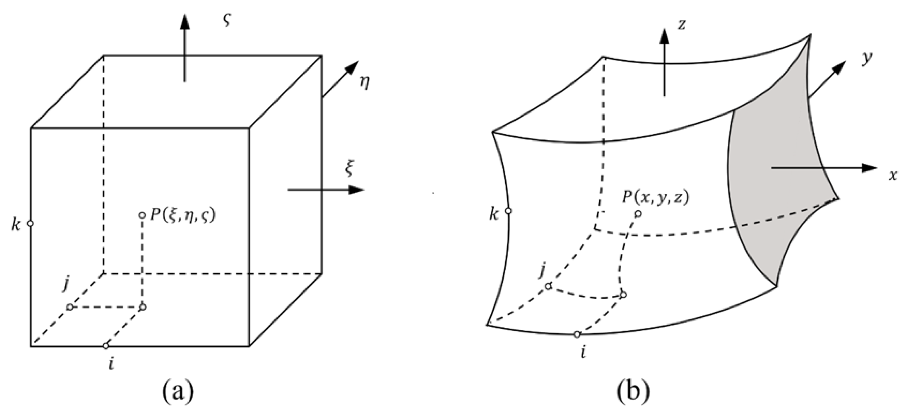
3.3. Mapping Differential Matrix

For three-dimensional problems, a hexahedron block with 20 seeds is selected in order to transform the coordination (x, y, z) to ( ξ , η , ζ ) as shown in Figure 3. The mapping function is expressed as
x = q = 1 20 N q ( ξ , η , ζ ) x q , y = q = 1 20 N q ( ξ , η , ζ ) y q , z = q = 1 20 N q ( ξ , η , ζ ) z q
The partial differentials of function u ( x , y , z ) with subject to axis ξ , η or ζ can be written as
u ξ = u x x ξ + u y y ξ + u z z ξ , u η = u x x η + u y y η + u z z η , u ζ = u x x ζ + u y y ζ + u z z ζ
Then the partial differentials of the function u ( x , y , z ) with respect to x, y and z are given by
u x = 1 | J | ( u ξ β 11 + u η β 12 + u ζ β 13 ) , u y = 1 | J | ( u ξ β 21 + u η β 22 + u ζ β 23 ) , u z = 1 | J | ( u ξ β 31 + u η β 32 + u ζ β 33 )
in which β i j express the terms in the cofactor of Jacobi matrix J, and
J = ( x ξ x η x ζ y ξ y η y ζ z ξ z η z ζ )
Therefore, the first order partial differential in the physical domain can be written as
u , x = ( Δ 11 D ξ + Δ 12 D η + Δ 13 D ζ ) u = D x u
u , y = ( Δ 21 D ξ + Δ 22 D η + Δ 23 D ζ ) u , = D y u
u , z = ( Δ 31 D ξ + Δ 32 D η + Δ 33 D ζ ) u , = D z u
in which
Δ i j = ( β i j ( 1 ) | J ( 1 ) | 0 0 0 β i j ( 2 ) | J ( 2 ) | 0 0 0 β i j ( M ) | J ( M ) | )
where β i j ( 1 ) / | J ( 1 ) | can be determined from Equation (27) at each node in the normalized domain, and the first order differentials matrix is determined by the Lagrange interpolation functions in normalized domain ( | ξ | 1 , | η | 1 , | ζ | 1 ) .

3.4. Mapping Technology with 3D Blocks

For the semi-infinite structure shown in Figure 4a, the semi-infinite domain is divided into several subdomains with two 20-seed-finite blocks, two 12-seed-one-infinite-edge blocks, two 7-seed-two-infinite-edge blocks and two 8-seed-three-infinite-edge blocks as shown in figures from Figure 4b–e. The infinite blocks in different directions can be obtained by rotating the initial mapping function. The mapping function for the finite block and infinite blocks in a general form is written as
N q = Q ( ξ , η , ζ , ξ q , η q , ζ q )
where q is the seed number shown in Figure 4. The details of the mapping function and their partial differentials can be presented in Appendix A in different categories.

4. Formulations for Bimodular Material with Meshless FBM

The equilibrium equation, in the domain, gives
σ + f = 0
where = { / x , / y , / z } , and stress tensor
σ = ( σ x x σ x y σ x z σ x y σ y y σ y z σ x z σ y z σ z z )   and   f = ( f x f y f z )
in which σ α β , ( α , β = x , y , z ) denotes stress; f α are body force. Substituting the constitutive equation, Equation (1), into the kinematic equation in Equation (33) without body forces yields
C 11 u x + C 12 u y + C 13 u z = 0 , C 21 u x + C 22 u y + C 23 u z = 0 , C 31 u x + C 32 u y + C 33 u z = 0 ,
where u x , u y , u z are vectors of nodal displacements, and C i j , ( i , j = 1 ,   2 ,   3 ) are coefficients by the constitutive and equilibrium equations, and given by
C 11 = Q 11 D x 2 + 2 Q 16 D x D y + 2 Q 15 D x D z + Q 66 D y 2 + 2 Q 56 D y D z + Q 55 D z 2 , C 22 = Q 66 D x 2 + 2 Q 26 D x D y + 2 Q 46 D x D z + Q 22 D y 2 + 2 Q 24 D y D z + Q 44 D z 2 , C 22 = Q 55 D x 2 + 2 Q 45 D x D y + 2 Q 35 D x D z + Q 44 D y 2 + 2 Q 34 D y D z + Q 33 D z 2 , C 12 = C 21 = Q 16 D x 2 + ( Q 21 + Q 66 ) D x D y + Q 26 D y 2 + ( Q 25 + Q 46 ) D y D z + Q 45 D z 2 , C 13 = C 31 = Q 15 D x 2 + ( Q 14 + Q 56 ) D x D y + ( Q 13 + Q 55 ) D x D z + Q 46 D y 2 + ( Q 36 + Q 45 ) D y D z + Q 35 D z 2 , C 23 = C 32 = Q 56 D x 2 + ( Q 25 + Q 46 ) D x D y + ( Q 36 + Q 45 ) D x D z + Q 24 D y 2 + ( Q 23 + Q 44 ) D y D z + Q 34 D z 2 ,
where Q i j , ( i , j = 1 ,   2 ,   , 6 ,   Q i j = Q j i ) are the terms in elasticity matrix Q and given by
Q = { Q 11 Q 12 Q 13 Q 14 Q 15 Q 16 Q 22 Q 23 Q 24 Q 25 Q 26 Q 33 Q 34 Q 35 Q 36 Q 44 Q 45 Q 46 Sym . Q 55 Q 56 Q 66 } .
Consider the following boundary conditions defined as
t ( x ) = t ¯ ( x ) , x Γ t u ( x ) = u ¯ ( x ) , x Γ u
where t ¯ ( x ) and u ¯ ( x ) are given traction and displacement on the boundary, t ¯ ( x ) = { t ¯ x , t ¯ y , t ¯ z } T , u ¯ ( x ) = { u ¯ x , u ¯ y , u ¯ z } T . x is the collocation point on the boundary. Traction t ¯ ( x ) can be rewritten as
B 11 u x + B 11 u x + B 11 u x = t ¯ x , B 21 u x + B 22 u x + B 23 u x = t ¯ y , B 31 u x + B 32 u x + B 33 u x = t ¯ z
where matrix B i j , ( i , j = 1 ,   2 ,   3 ) is associated with the boundary collocation point
B 11 = D x ( Q 11 n x + Q 16 n y + Q 15 n z ) + D y ( Q 16 n x + Q 66 n y + Q 56 n z ) + D z ( Q 15 n x + Q 56 n y + Q 55 n z ) , B 22 = D x ( Q 66 n x + Q 26 n y + Q 46 n z ) + D y ( Q 26 n x + Q 22 n y + Q 24 n z ) + D z ( Q 46 n x + Q 24 n y + Q 44 n z ) , B 33 = D x ( Q 55 n x + Q 45 n y + Q 35 n z ) + D y ( Q 45 n x + Q 44 n y + Q 34 n z ) + D z ( Q 35 n x + Q 34 n y + Q 33 n z ) , B 12 = D x ( Q 16 n x + Q 66 n y + Q 56 n z ) + D y ( Q 12 n x + Q 26 n y + Q 25 n z ) + D z ( Q 14 n x + Q 46 n y + Q 45 n z ) , B 13 = D x ( Q 15 n x + Q 56 n y + Q 55 n z ) + D y ( Q 14 n x + Q 46 n y + Q 45 n z ) + D z ( Q 13 n x + Q 36 n y + Q 35 n z ) , B 21 = D x ( Q 16 n x + Q 12 n y + Q 14 n z ) + D y ( Q 66 n x + Q 26 n y + Q 46 n z ) + D z ( Q 56 n x + Q 25 n y + Q 45 n z ) , B 23 = D x ( Q 56 n x + Q 25 n y + Q 45 n z ) + D y ( Q 46 n x + Q 24 n y + Q 44 n z ) + D z ( Q 36 n x + Q 23 n y + Q 34 n z ) , B 31 = D x ( Q 15 n x + Q 14 n y + Q 13 n z ) + D y ( Q 56 n x + Q 46 n y + Q 36 n z ) + D z ( Q 55 n x + Q 45 n y + Q 35 n z ) , B 32 = D x ( Q 56 n x + Q 46 n y + Q 36 n z ) + D y ( Q 25 n x + Q 24 n y + Q 23 n z ) + D z ( Q 35 n x + Q 34 n y + Q 33 n z )
where n α , ( α = x , y , z ) is the boundary outwards normal. Therefore, 3 × M linear algebraic equations are obtained in total from Equations (33) and (38). In addition, on the interfaces between blocks, the following continued conditions should be taken into account
u α ( i ) u α ( j ) = 0 , t α ( i ) + t α ( j ) = 0 , ( α = x , y , z ) ,
where u α ( i ) and t α ( i ) represent the displacement and traction on the interface between block i and block j. Finally, a set of linear algebraic equations is established the in global system as follows
K [ 3 M × 3 M ] U [ 3 M × 1 ] = F [ 3 M × 1 ] ,
Where K is the stiffness matrix, U is the vector of displacements and F is the vector consisting of the boundary value of the displacement, tractions and domain body forces. The following nonlinear iterative algorithm is adopted in this paper.
Step 1: m = 0, take either tensile or compressive modulus at all collocation points. Solve the global stiffness matrix to obtain the initial displacements, stresses and strains.
Step 2: Determine the principal stress σ α , σ β , σ γ and the direction at each node. Then, determine the moduli, Poisson’s ratios ( E + , E ), ( v + , v ) and the constitutive matrix according from Equations (6)–(14).
Step 3: Modify the stiffness matrix K and vector F based on the current step. Solve the equations again to obtain the displacements, stresses and strains at each node.
Step 4: Calculate the average error from all collocation points
κ = 1 M i = 1 M | U i ( m ) U i ( m 1 ) |
where U i ( m ) presents the displacement at step m. if κ < 10 6 , terminate the iteration and print out the result. Otherwise, let m = m + 1; go to step 2.

5. Numerical Examples

In this section, four examples are presented to demonstrate the accuracy of the meshless FBM with bimodular materials. A 3D tensile column with gravity is investigated in the first example. Then, FBM is applied to an arch bridge model, a single-layer semi-infinite model and a multi-layer pavement foundation under different loadings. All codes were written with Matlab (R2021b, The MathWorks, Inc., Natick, MA, USA).and Fortran in subroutine UMAT using ABAQUS (2019, Dassault Systèmes Simulia Corp., Vélizy-Villacoublay, France).

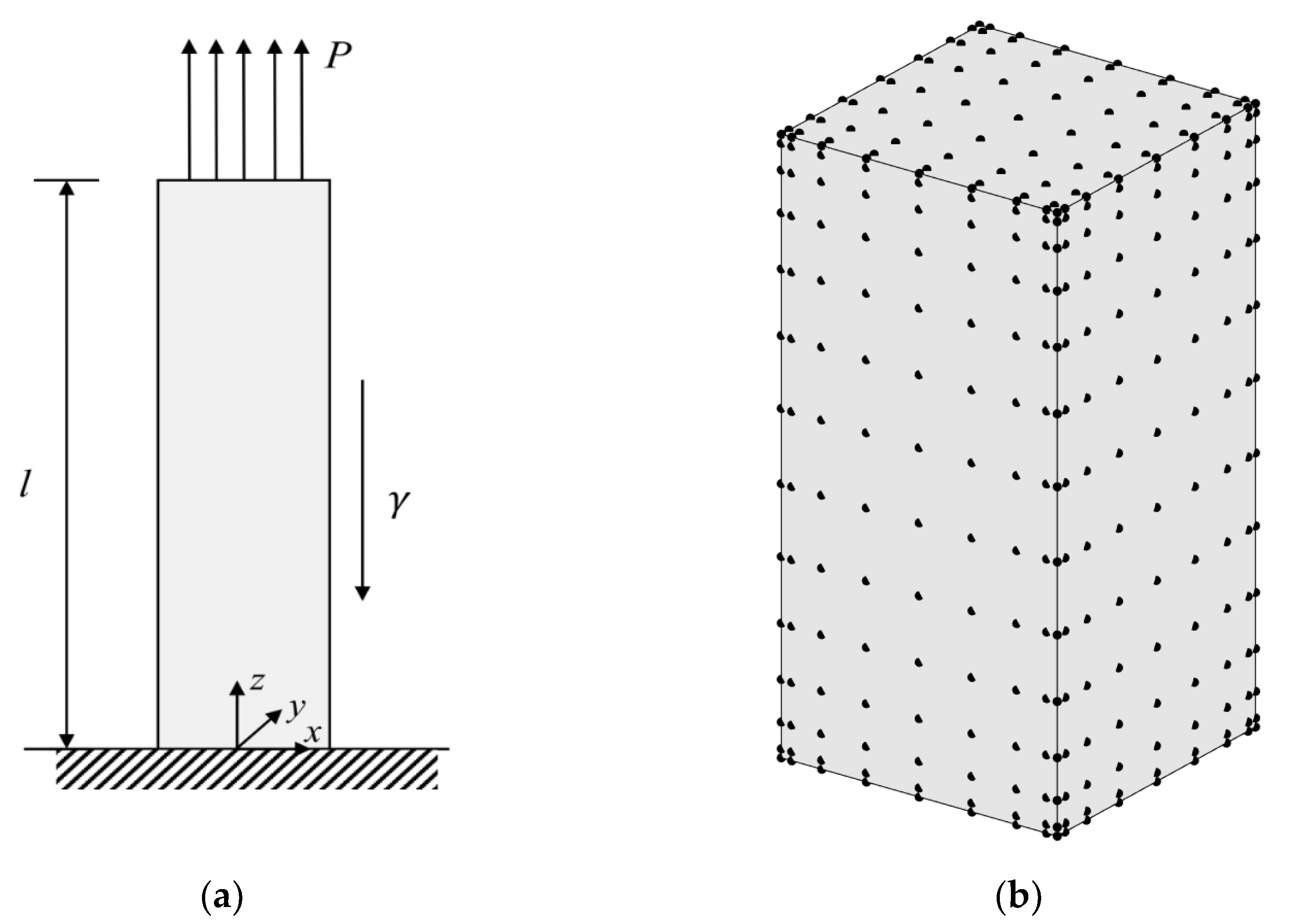
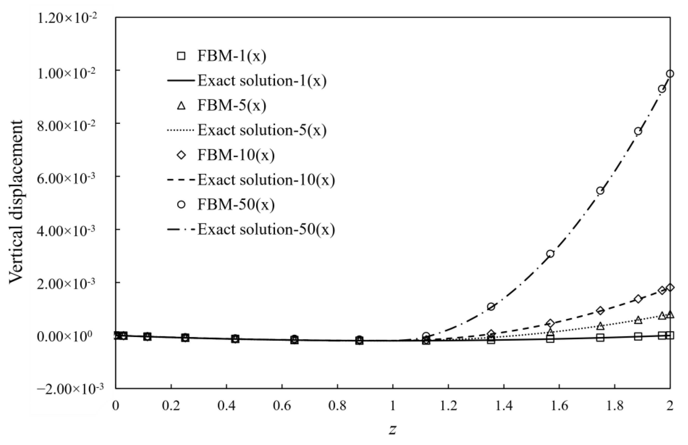
5.1. Tensile Column with Gravity

Consider a gravitational column of the length l = 2; the dimension of the cross-section is normalized as 1 × 1, and the mass density γ = 2 as shown in Figure 5a. It is fixed on the bottom and a tensile force P of 2 units is applied to the top. It is assumed that a compression modulus is 5000 units, and the Poisson’s ratios in tension and compression is zero. The exact solution of the displacement [1] along the z-axis is given as
ω = { P z E γ E ( l z 1 2 z 2 ) , z < c γ 2 [ ( z c ) 2 E + c 2 E ] , z c
where c = l P / γ . The numbers of node in x-axis and y-axis are 9, and in the z-axis is 14. The locations of node along different axes in the normalized domain are chosen
ξ i = c o s π ( i 1 ) N ξ 1 , i = 1 , 2 , , N ξ ; η j = c o s π ( j 1 ) N η 1 , j = 1 , 2 , , N η ; ζ k = c o s π ( k 1 ) N ζ 1 , k = 1 , 2 , , N ζ
The total number of nodes for the FBM is 1134 (= 9 × 9 × 14), and 396 C3D20R elements are used in FEM. The node distribution of FBM is shown in Figure 5b. Comparison between the exact solution and FBM solution at point z = 1.96 and the number of iterations for convergence between FEM and FBM are presented in Table 1. With different ratios of tensile and compression modulus, the vertical displacement changes along the z-axis and exact solution are shown in Figure 6. Obviously, the FBM can give an accurate solution for the problem and shows a similar convergence rate when compared with the FEM method. To investigate the accuracy for different node density, the average relative errors are defined as
ε = 1 M q = 1 M | ω ω * |
The numerical results presented in Table 2 demonstrate the average errors with iteration numbers of convergence over all collocation points when E / E + = 10 . Observing the results in Table 2, it is evident that increasing the node density improves the degrees of accuracy, and convergency is easily approached in iterations when the node number N ξ is more than 3.

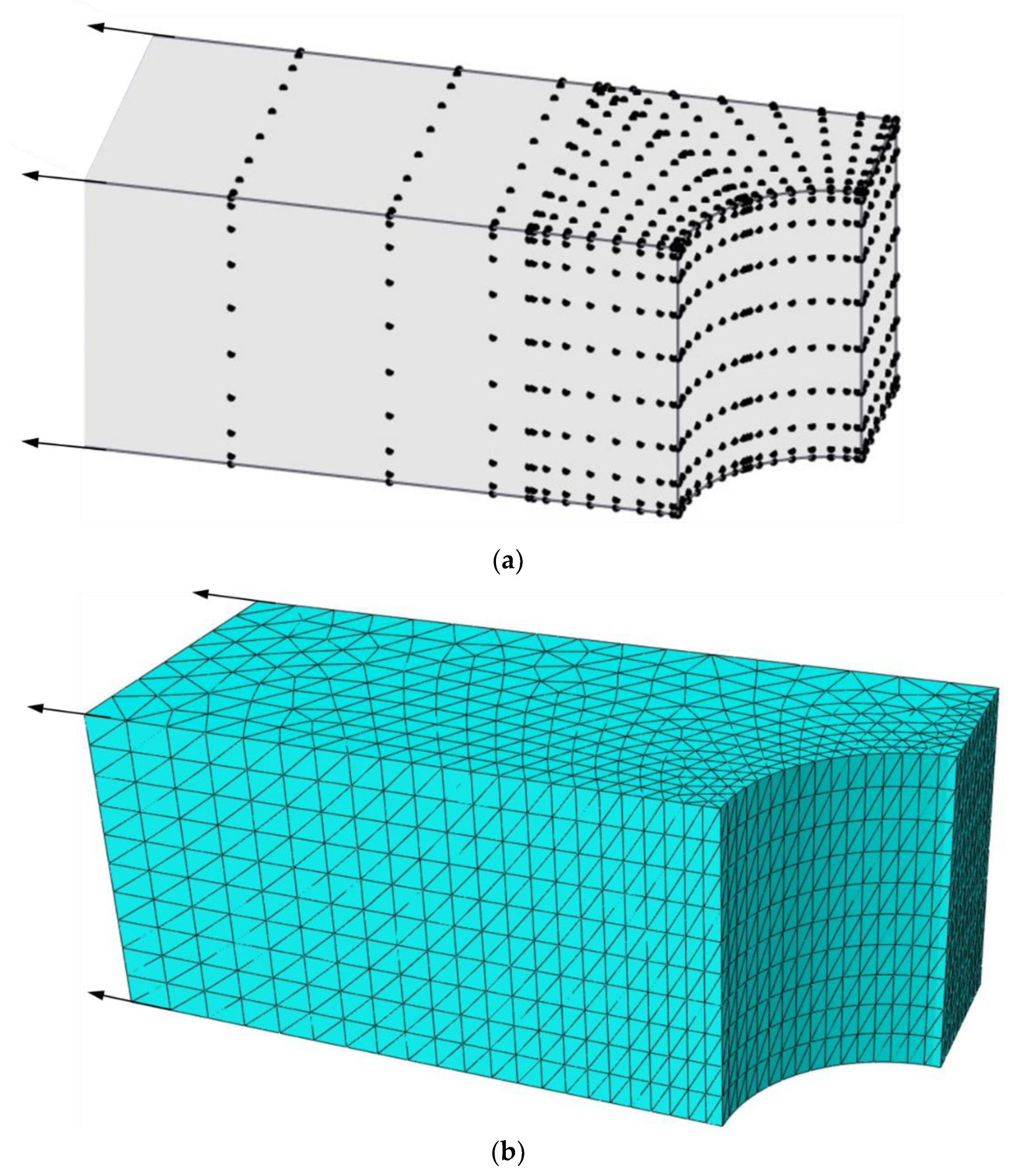
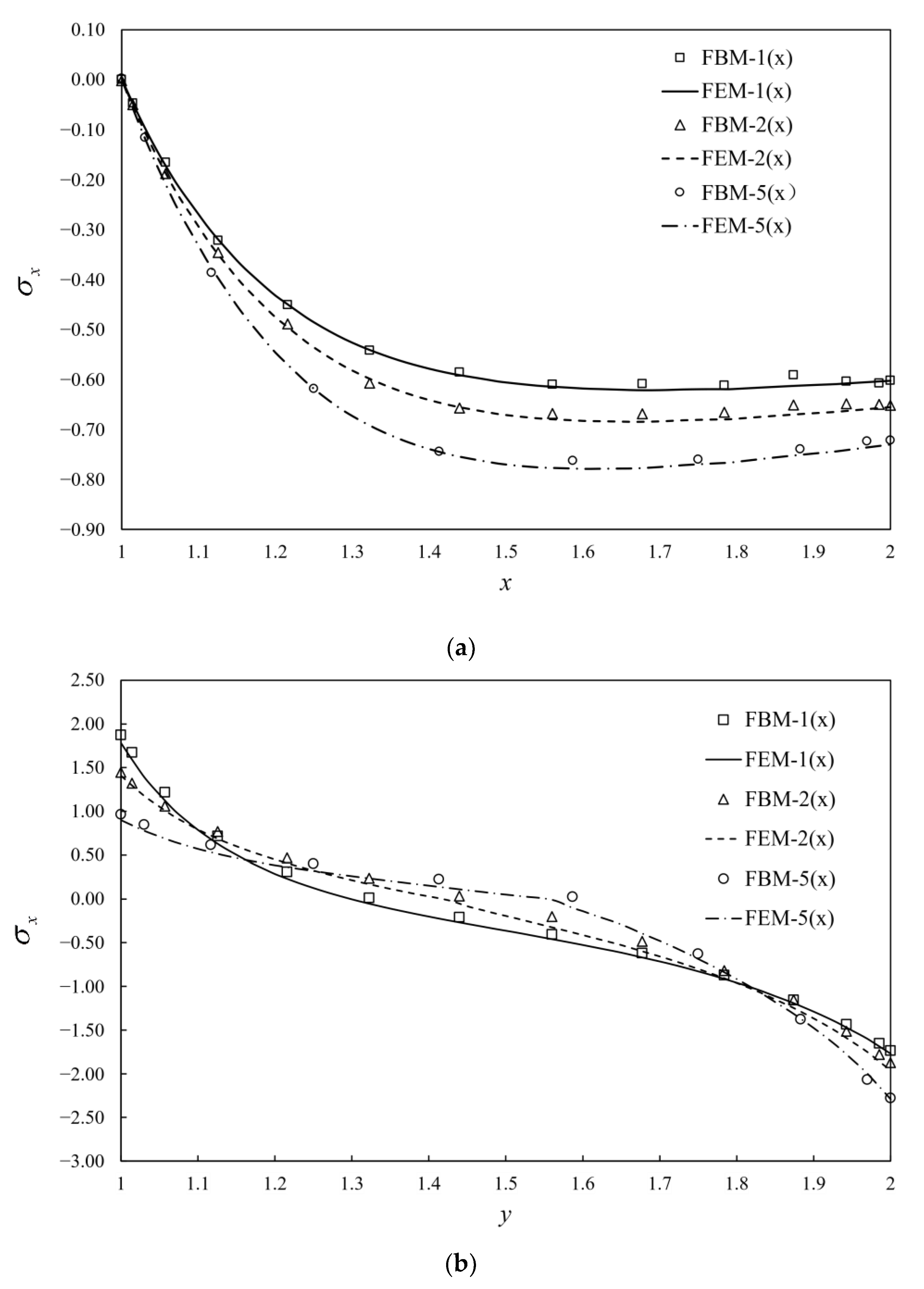
5.2. Arch Bridge in Bimodular Materials

Consider a simplified arch bridge as shown in Figure 7. Due to the symmetry of the structure, half of the model is taken for analysis. The radius of the arc is a = 1 unit. There is a vertical pressure load p 0 of 1 unit applied on the top, and the lengths in both y-axis and x-axis are w(=2a). The displacement u y is fixed on the bottom face (y = 0), and u x is zero on the surface x = 0. The ratios of Young’s moduli are selected as E / E + = 1 ,   2 ,   5 , compression modulus E = 1 unit and Poisson’s ratio v = 0.4 in the computation procedure.
The bridge is divided into three blocks using FBM shown in Figure 7, where blocks I and II are finite blocks with 20-seed and block III is one semi-infinite block with a 12-seed-one-infinite-edge. In the discretization of each block, there are 12 and 14 collocation nodes along finite and infinite directions, respectively. The distribution of nodes along each axis is the same as Equation (45) in Section 5.1, as shown in Figure 8a. Stresses along two segments, AB and CD, shown in Figure 7 are plotted to illustrate the degree of accuracy. Simulation with FEM is complemented with 90,912 C3D10 elements as shown in Figure 8b. The length in the x-axis is w = 40 unit. The normalized stress σ x along AB, CD and AC by FBM and FEM is plotted in Figure 9 to show the difference between these two methods with bimodular materials. Reasonable agreements can clearly be observed. It is also noticed that there are several kinks in Figure 9 for stress distributions by the FEM due to the discontinuity of the Young’s modulus.
.

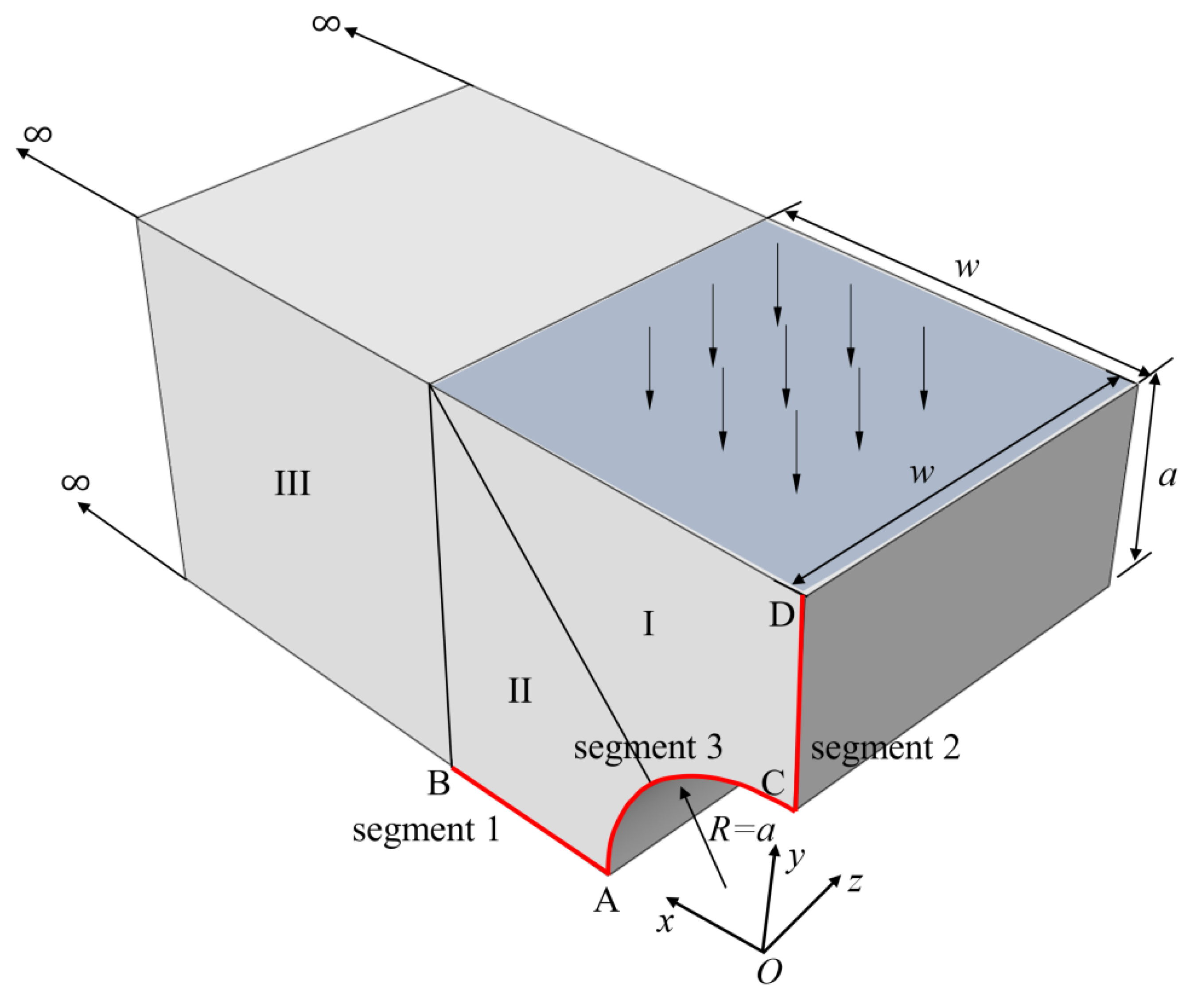
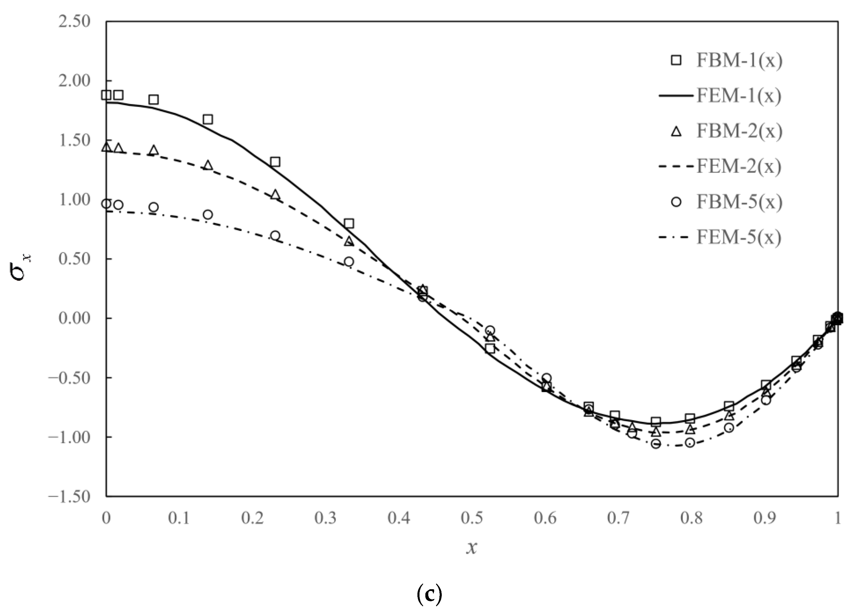
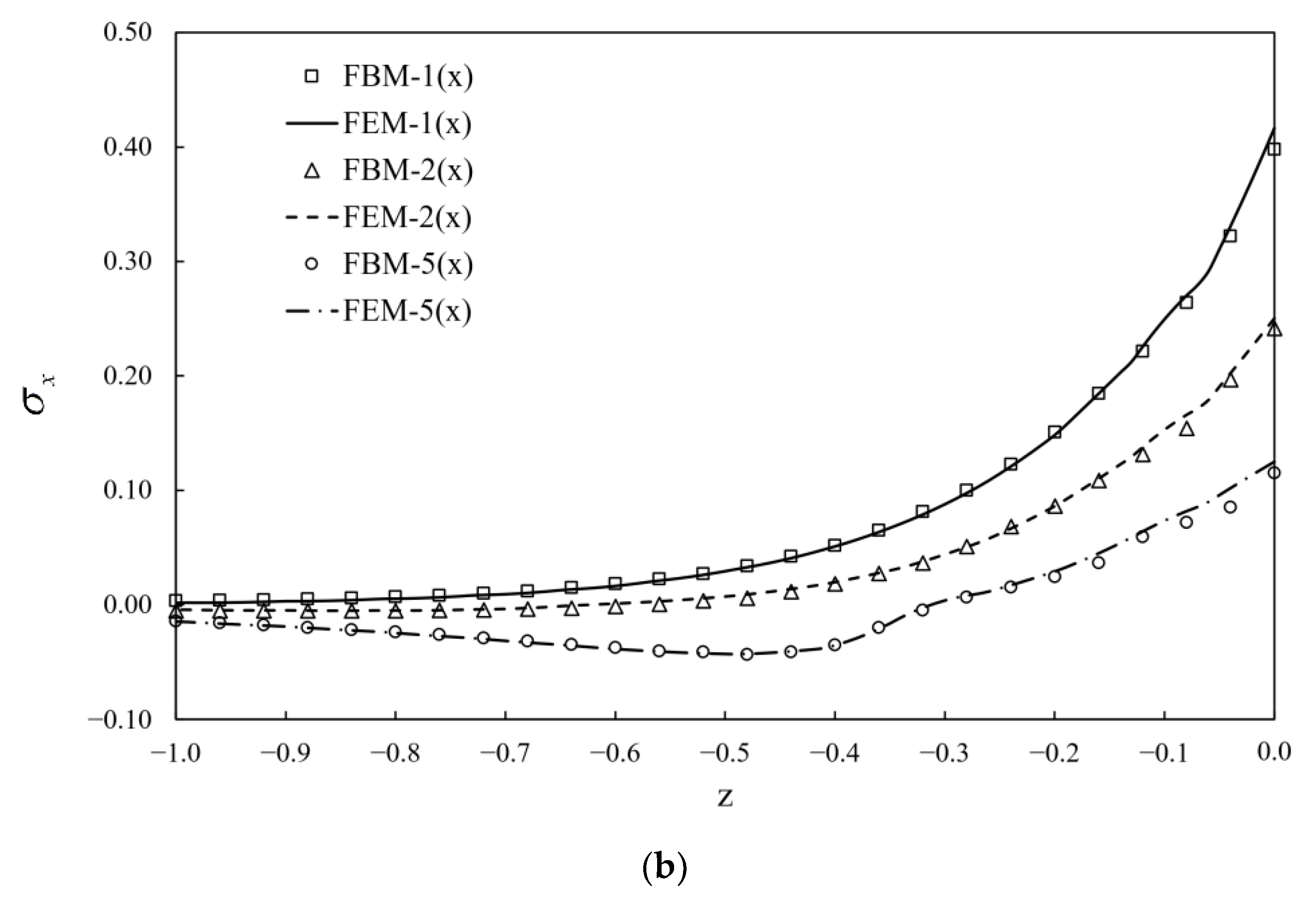
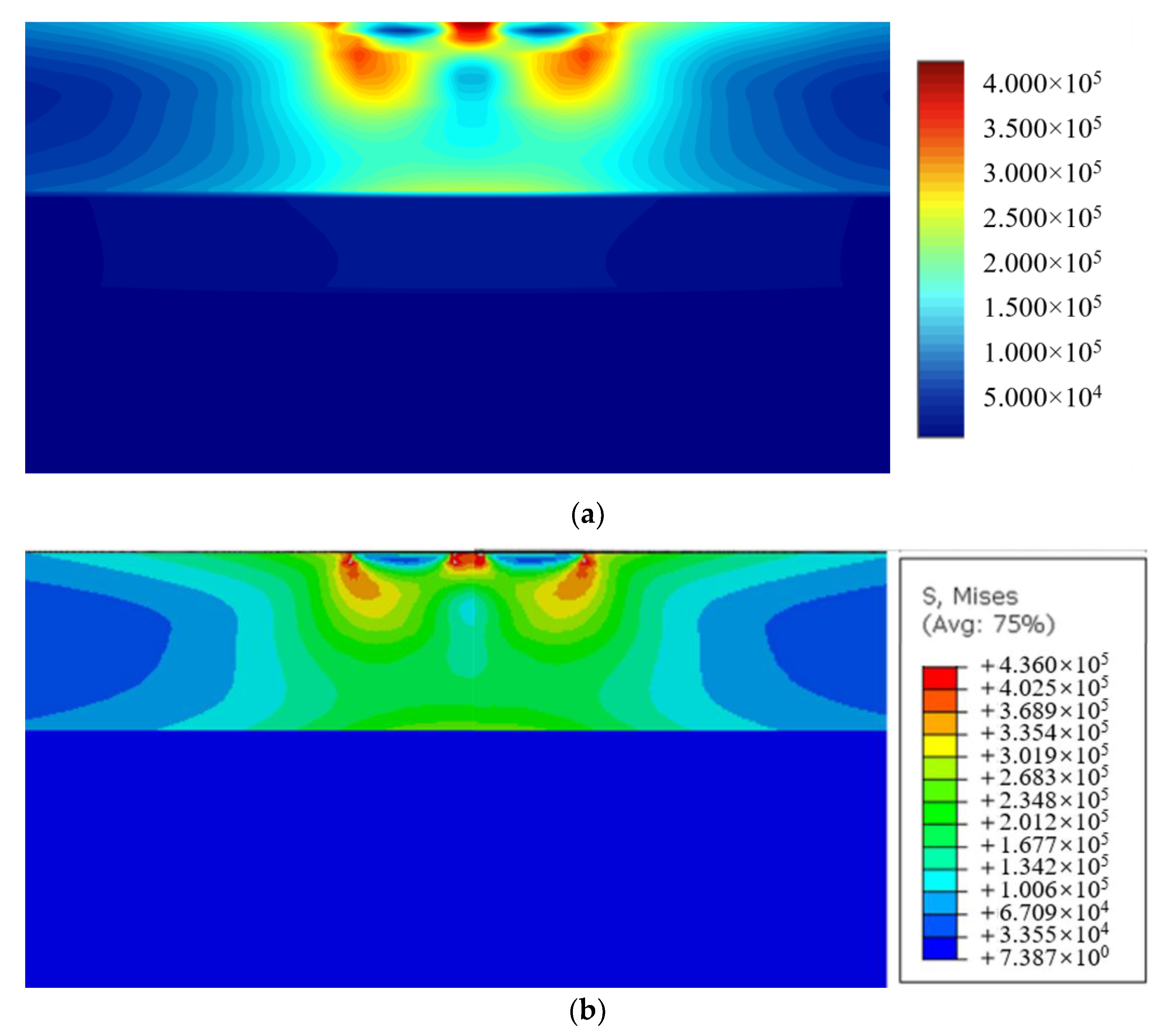
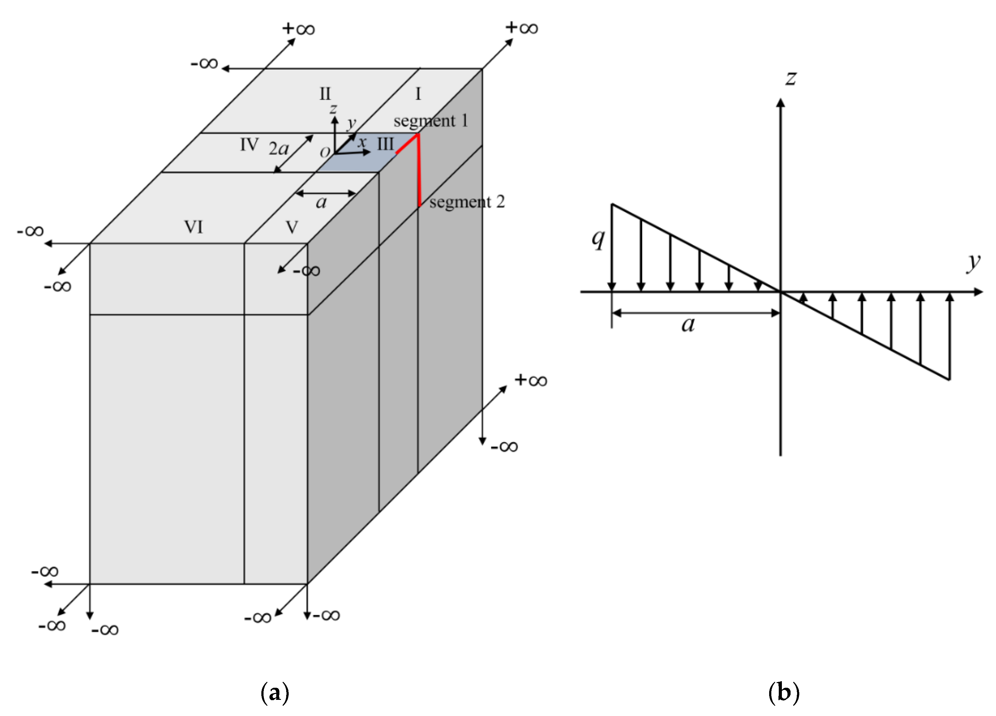
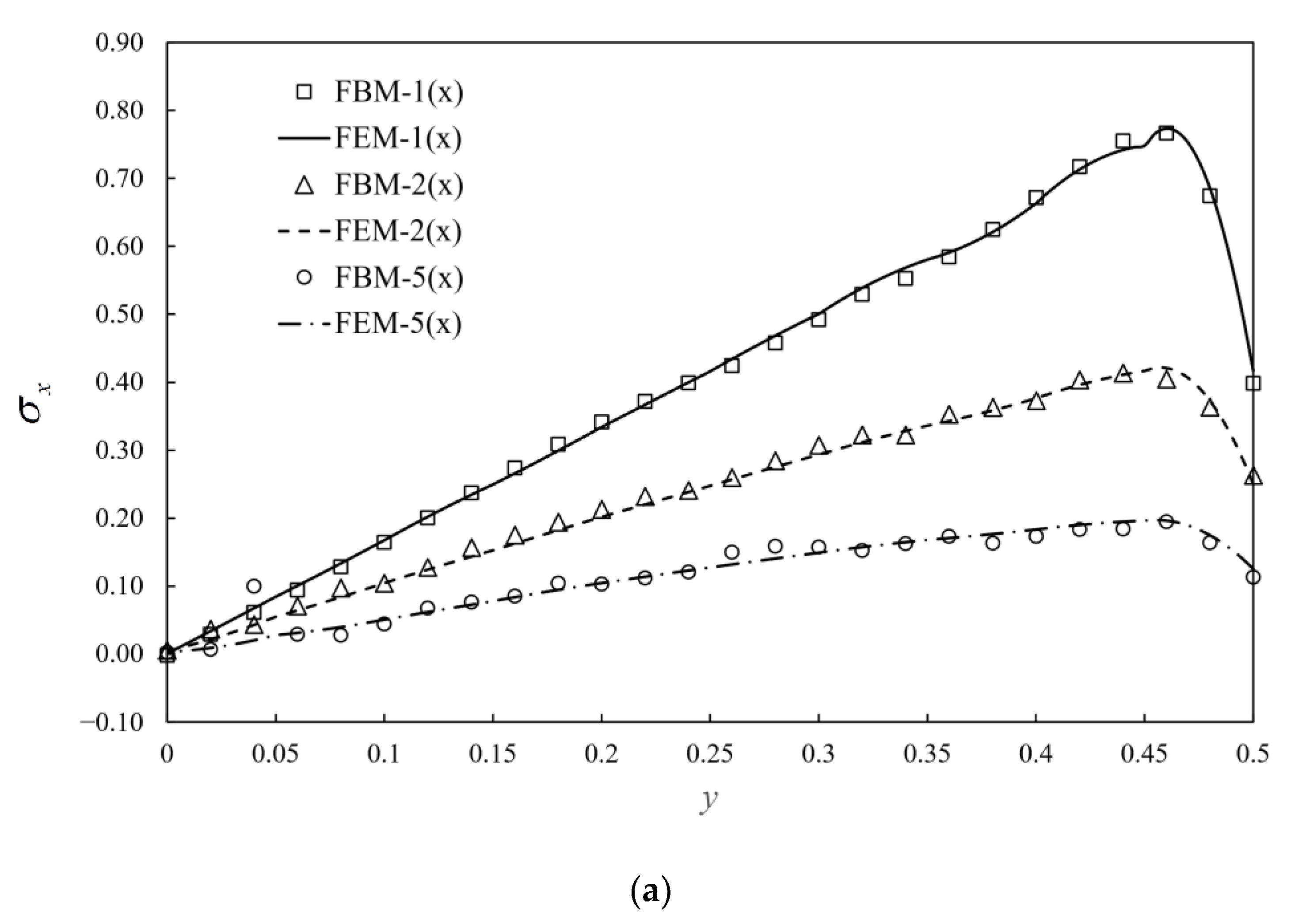
5.3. A Semi-Infinite Solid with Bimodular Materials

The semi-infinite structures are introduced to simulate soil foundations. Consider a semi-infinite body as shown in Figure 10a with the linear distributed vertical load in a square area of width 1 unit on the surface. The linear distributed load is plotted in Figure 10b with a unit maximum absolute value of q in compression and tension. Bimodular materials are selected with three different ratios of tensile and compressive moduli, as shown in Table 3. Due to the symmetry of the structure and loading, only a half model is analyzed as shown in Figure 10a. To accurately capture the stress near the loading area, the structure is subdivided into two layers. The first layer includes one 20-seed finite block III, three 12-seed-one-infinite-edge blocks I, IV, V and two 7-seed-two-infinite-edge block II and VI. However, in the second layer, one 12-seed-one-infinite-edge block, three 7-seed-two-infinite-edge blocks and two 8-seed-three-infinite-edges blocks are used. For each block, 9 collocation points are used on the finite edge and 12 points for the infinite edge. Normalized stress σ x along AB and AC are presented to demonstrate the accuracy of the FBM shown in Figure 11a,b versus the different ratios of tensile and compressive moduli, and Poisson ratios. In this example, FEM simulation is complemented by use of 362,484 C3D10 elements with dimensions of 20 units in length and height and 10 units in the width. A reasonable agreement was clearly achieved.

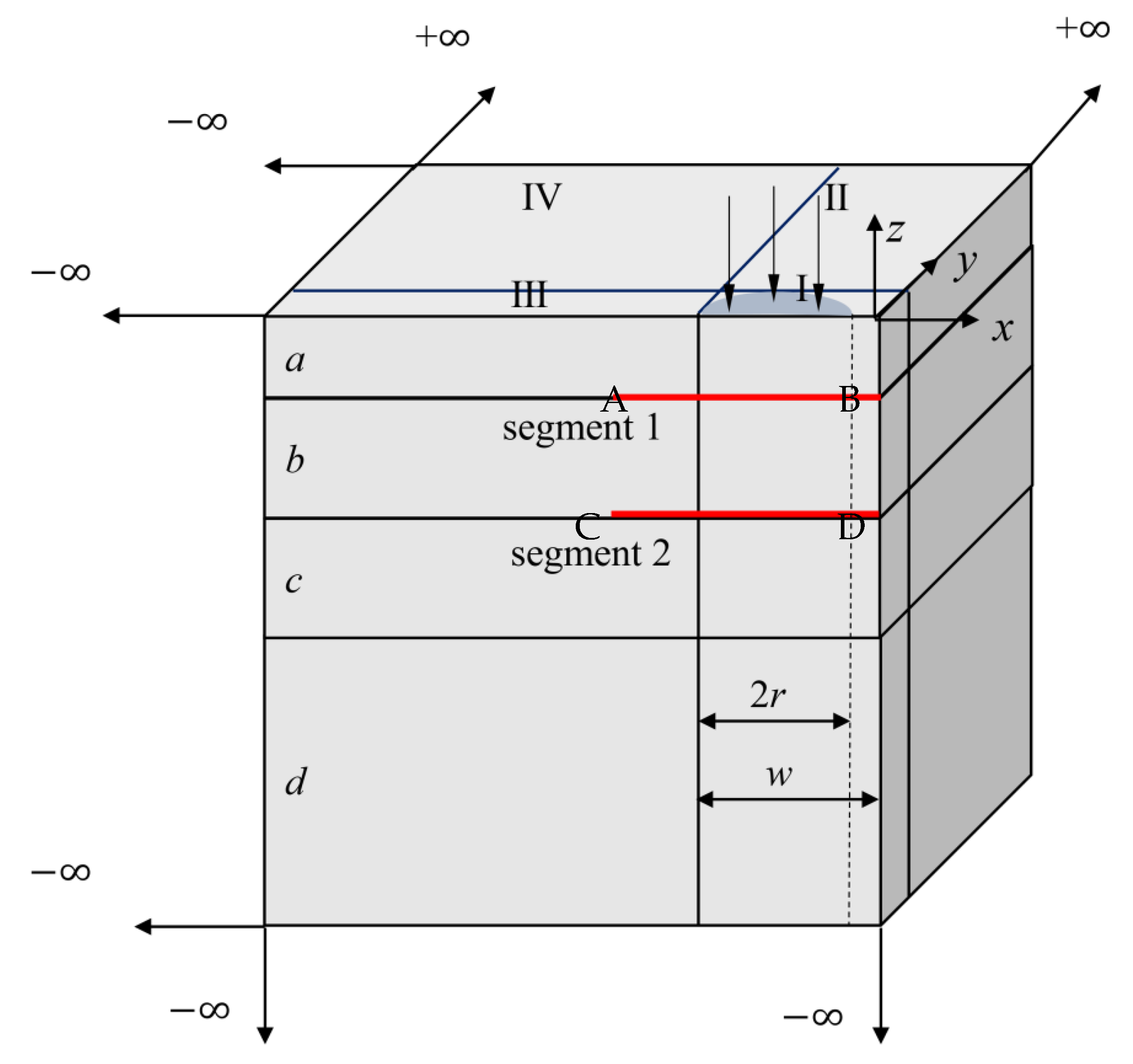
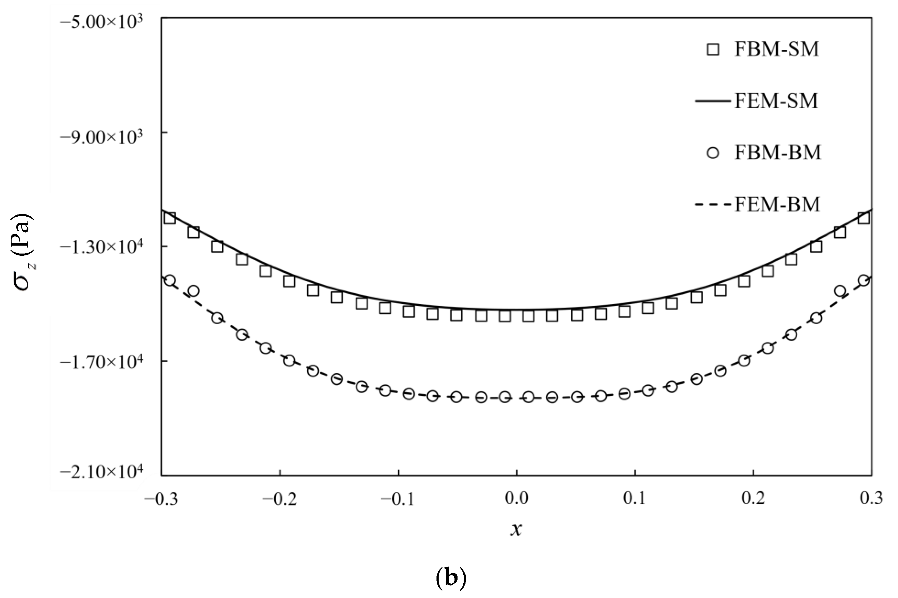
5.4. Multi-Layered Infinite Model with Bimodular Materials

Consider a multi-layered infinite structure, as shown in Figure 12, to simulate a highway pavement structure under two symmetric circular pressure loads. The pressure is assumed to be 0.7 MPa with a radius of 0.1065 m. The distance between two centers of loads is 0.3195 m. The model contains four layers; the first and second layers are bimodulus materials and the third and fourth layers are isotropic materials. The details of material parameters and dimensions of each layer are listed in Table 4. Again, due to the symmetry of the structure and load condition, quarter of the structure is analyzed as shown in Figure 12. During the numerical process, each layer is divided into four blocks. For the first layer, the top layer contains one 20-seed finite block, two 12-seed-infinite-edge blocks II and III and one 7-node-two-infinite-edge block IV. In the second and third layers, the same block distribution is applied as in the first layer. The bottom layer contains one 12-seed-one-infinite-edge block I, two 7-seed-two-infinite-edge blocks II and III and one 8-seed-three-infinite-edge block IV.
Like the node distributions in Section 5.3, the 8 seeds are used on the finite edges and 14 seeds on the infinite edges. The total number of collocation nodes by FBM is 12288. To validate the computational accuracy, the results of stresses σ z by FBM and FEM along segment AB and segment CD are compared in Figure 13. The contours of von Mises stress with bimodular materials on y = 0 are presented by using FBM in Figure 14. FEM is also used for analysis with no dimension of 20 × 20 × 20 and 127,760 C3D20R elements used in this example. It can be seen that the position of the maximum von Mises stress with these two methods is the almost the same, and the values are also very close to each other. In addition, the FBM results are smoother.

6. Conclusions

A meshless finite block method with infinite block analyzing three-dimensional solids of bimodular materials was demonstrated in this paper. A mapping technique was applied to determine the first order of derivatives. The 20-node finite block, 12-seed-one-edge-infinite block, 7-seed-two-edge-infinite block and 8-seed-three-edge-infinite block were introduced to simulate all semi-infinite domains. An iterative process for the meshless finite block method with a shear-modulus-complemented algorithm to solve bimodular problems was proposed. The numerical algorithm was validated with four examples. The finite element software ABAQUS was used for comparison. The following conclusions can be summarized: (1) FBM easily tackles nonlinear problems with semi-infinite boundaries; (2) a shear modulus algorithm efficiently and accurately describes the bimodular mechanical behavior of materials; (3) the proposed method shows efficiency and accuracy for semi-infinite problems with bimodular materials. Compared to FEM, FBM is more accurate with the same computational effort; (4) FBM can be applied to more complicated problems, such as 3D elastoplasticity, thermoelasticity and elastodynamics.
FE methods are rather general and efficient numerical tools to deal with complicated problems in engineering. However, as an alternative, the meshless finite block method with an infinite-mapping technique provides a new approach in solving unbounded bimodular material problems, with many advantages including efficiency and simplicity. As ABAQUS is a commercialized package, the CPU times used by different approaches are not comparable in this work. At present, dividing blocks is still a manual process in FBM; the versatility needs to be further improved with complex regional models. In future work, the FBM is expected to be extended to apply to more complicated problems, such as 3D elastoplasticity, thermoelasticity and elastodynamics.

Author Contributions

Data curation, W.H. and J.S.; Investigation, J.Y. and P.W.; Methodology, P.W. and V.S.; Resources, J.Y.; Software, W.H. and V.S.; Validation, J.S. All authors have read and agreed to the published version of the manuscript.

Funding

This work was supported by the National Natural Science Foundation of China (grant numbers: 51478053), and the Hunan Provincial Postgraduate Research Innovation Project (grant numbers: QL20210183). The authors J.S. and V.S. acknowledge the support from the Slovak Science and Technology Assistance Agency registered under number APW-18-0004 and by the grant agency VEGA-2/0061/20.

Institutional Review Board Statement

Not applicable.

Informed Consent Statement

Not applicable.

Data Availability Statement

The data presented in this study are available on request from the corresponding author.

Acknowledgments

This work was supported by the National Natural Science Foundation of China (grant numbers: 51478053), and the Hunan Provincial Postgraduate Research Innovation Project (grant numbers: QL20210183). The authors J.S. and V.S. acknowledge the support from the Slovak Science and Technology Assistance Agency registered under number APW-18-0004 and by the grant agency VEGA-2/0061/20.

Conflicts of Interest
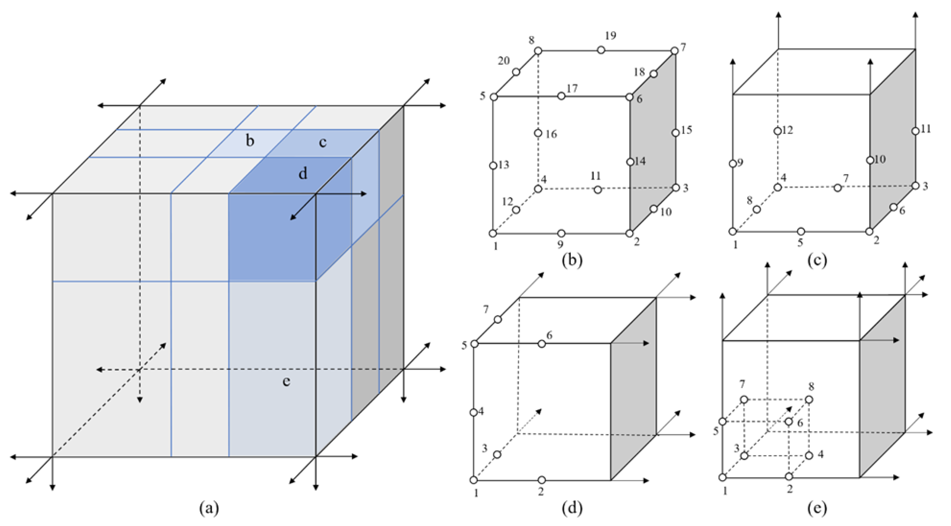
The authors declare no conflict of interest.

Appendix A

1.
20-node finite block
For this type of finite element, the physical domain is mapped to a cube with 20 seeds in coordination system ( ξ , η , ζ ) in the region | ξ | 1 , | η | 1 and | ζ | 1 , as shown in Figure 4b. The mapping function can be written as follows [51]:
N i = 1 8 ( 1 + ξ i ξ ) ( 1 + η i η ) ( 1 + ζ i ζ ) ( ξ i ξ + η i η + ζ i ζ 2 ) , i = 1 , 2 , 3 , 4 , 5 , 6 , 7 , 8 ,
N i = 1 4 ( 1 ξ 2 ) ( 1 + η i η ) ( 1 + ζ i ζ ) , i = 9 , 11 , 17 , 19 ,
N i = 1 4 ( 1 η 2 ) ( 1 + ζ i ζ ) ( 1 + ξ i ξ ) , i = 10 , 12 , 18 , 20 ,
N i = 1 4 ( 1 ζ 2 ) ( 1 + ξ i ξ ) ( 1 + η i η ) , i = 13 , 14 , 15 , 16 .
Their partial differentials of the mapping function are listed below:
N i ξ = ξ i 8 ( 1 + η i η ) ( 1 + ζ i ζ ) ( 2 ξ i ξ + η i η + ζ i ζ 1 ) , N i η = η i 8 ( 1 + ξ i ξ ) ( 1 + ζ i ζ ) ( ξ i ξ + 2 η i η + ζ i ζ 1 ) , N i ζ = ζ i 8 ( 1 + ξ i ξ ) ( 1 + η i η ) ( ξ i ξ + η i η + 2 ζ i ζ 1 ) , i = 1 , 2 , 3 , 4 , 5 , 6 , 7 , 8
N i ξ = 1 2 ξ ( 1 + η i η ) ( 1 + ζ i ζ ) , N i η = 1 4 η i ( 1 ξ 2 ) ( 1 + ζ i ζ ) , N i ξ = 1 4 ζ i ( 1 + η i η ) ( 1 + ξ 2 ) , i = 9 , 11 , 17 , 19
N i ξ = 1 4 ξ i ( 1 + η 2 ) ( 1 + ζ i ζ ) , N i η = 1 2 η ( 1 + ξ i ξ ) ( 1 + ζ i ζ ) , N i ξ = 1 4 ζ i ( 1 η 2 ) ( 1 + ξ i ξ ) , i = 10 , 12 , 18 , 20
N i ξ = 1 4 ξ i ( 1 ζ 2 ) ( 1 + η i η ) , N i η = 1 4 η i ( 1 ζ 2 ) ( 1 + ξ i ξ ) , N i ξ = 1 2 ζ ( 1 + η i η ) ( 1 + ξ i ξ ) , i = 13 , 14 , 15 , 16
2.
12-seed-one-edge-infinite block
In the normalized domain, the face of the upper side ( ζ = 1 ) is mapped to infinite area as shown in Figure 4c. The mapping functions [17] are
N i = 1 2 ( 1 + ξ i ξ ) ( 1 + η i η ) ( ξ i ξ + η i η ζ 2 ) / ( 1 ζ ) , i = 1 , 3 , 5 , 7 ,
N i = ( 1 ξ 2 ) ( 1 + η i η ) / ( 1 ζ ) , i = 2 , 6 ,
N i = ( 1 + ξ i ξ ) ( 1 η 2 ) / ( 1 ζ ) , i = 4 , 8 ,
N i = 1 4 ( 1 + ξ i ξ ) ( 1 + η i η ) ( 1 + ζ ) / ( 1 ζ ) , i = 9 , 10 , 11 , 12 .
The Cartesian coordinate system in the physical domain can be obtained
x = k = 1 12 N k ( ξ , η , ζ ) x k , y = k = 1 12 N k ( ξ , η , ζ ) y k , z = k = 1 12 N k ( ξ , η , ζ ) z k .
The first-order partial differentials of Equations (A9)–(A12) are
N i ξ = 1 2 ξ i ( 1 + η i η ) ( 1 + η i η + 2 ξ i ξ ζ ) / ( 1 ζ ) , N i η = 1 2 η i ( 1 + ξ i ξ ) ( 1 + ξ i ξ + 2 η i η ζ ) / ( 1 ζ ) , N i ζ = 1 2 ( 1 + ξ i ξ ) ( 1 + η i η ) ( 3 + η i η + ξ i ξ ζ ) / ( 1 + ζ ) 2 , i = 1 , 3 , 5 , 7
N i ξ = 2 ξ ( 1 + η i η ) / ( 1 ζ ) , N i η = η i ( 1 ξ 2 ) / ( 1 ζ ) , N i ζ = ( 1 + η i η ) ( 1 ξ 2 ) / ( 1 ζ ) 2 , i = 2 , 6
N i ξ = ξ i ( 1 + η 2 ) / ( 1 ζ ) , N i η = 2 η ( 1 + ξ i ξ ) / ( 1 ζ ) , N i ζ = ( 1 η 2 ) ( 1 + ξ i ξ ) / ( 1 ζ ) 2 , i = 4 , 8
N i ξ = 1 4 ξ i ( 1 + η i η ) ( 1 + ζ ) / ( 1 ζ ) , N i η = 1 4 ( 1 + ξ i ξ ) η i ( 1 + ζ ) / ( 1 ζ ) , N i ζ = 1 2 ( 1 + η i η ) ( 1 + ξ i ξ ) / ( 1 + ζ ) 2 , i = 9 , 10 , 11 , 12
3.
7-seed-two-edge-infinite block
In this case, two edges ( ξ = 1 , η = 1 ) in the normalized domain is mapped to infinite place as shown in Figure 4d. The shape functions [17,52] are
N 1 = ( 1 ξ ) ( 5 ξ η 4 ζ + 3 ξ η ) / ( 2 α ) , N 2 = ( 1 ζ ) ( 1 + ξ ) [ 2 ( 1 ξ ) ] , N 3 = ( 1 ζ ) ( 1 + η ) [ 2 ( 1 ξ ) ] , N 4 = 4 ( 1 ζ 2 ) α , N 5 = ( 1 + ζ ) ( 5 ξ η + 4 ζ + 3 ξ η ) / ( 2 α ) , N 6 = ( 1 + ζ ) ( 1 + ξ ) [ 2 ( 1 ξ ) ] , N 7 = ( 1 ζ ) ( 1 + ξ ) [ 2 ( 1 η ) ] ,
in which α = ( 1 ξ ) ( 1 η ) with coordinate transformation
x = k = 1 7 N k ( ξ , η , ζ ) x k , y = k = 1 7 N k ( ξ , η , ζ ) y k , z = k = 1 7 N k ( ξ , η , ζ ) z k .
Their partial differential with respect to ξ , η and ζ are given as follows:
N 1 ξ = ( 1 ζ ) ( 3 η + 2 ζ ) / β , N 2 ξ = ( 1 ζ ) / ( 1 ξ ) 2 , N 3 ξ = N 7 ξ = 0 , N 4 ξ = 4 ( 1 ζ 2 ) / β , N 5 ξ = ( 1 + ξ ) ( 3 + η + 2 ζ ) / β , N 6 ξ = ( 1 + ζ ) / ( 1 ξ ) 2 ,
N 1 η = ( 1 ζ ) ( 3 + ξ 2 ζ ) / γ , N 2 η = N 6 η = 0 , N 3 η = ( 1 ξ ) / ( 1 η ) 2 , N 4 η = 4 ( 1 ζ 2 ) / γ , N 5 η = ( 1 + ζ ) ( 3 + η + 2 ζ ) / γ , N 7 η = ( 1 + ζ ) / ( 1 η ) 2 ,
N 1 ζ = ( 1 ξ + η 3 ξ η + 8 ζ ) / ( 2 α ) , N 2 ζ = ( 1 + ξ ) / [ 2 ( 1 ξ ) ] , N 3 ζ = ( 1 + η ) / [ 2 ( 1 η ) ] , N 4 ζ = 8 ζ / α , N 5 ζ = ( 1 ξ η + 3 ξ η + 8 ζ ) / ( 2 α ) , N 6 ζ = ( 1 + ξ ) / [ 2 ( 1 ξ ) ] N 7 ζ = ( 1 + η ) / [ 2 ( 1 η ) ] ,
where α = ( 1 ξ ) ( 1 η ) , β = α ( 1 ξ ) , γ = α ( 1 η ) .
4.
8-seed-three-edge-infinite block
This type of infinite element is extended from Lagrangian 27-node brick, which is shown in Figure 4e. Three directions ( ξ = 1 , η = 1 , ζ = 1 ) in the normalized domain are mapped to infinity. The shape functions [17,52] are simplified
N 1 = 8 ξ η ζ / α , N 2 = 4 η ζ ( 1 + ξ ) / α , N 3 = 4 ξ ζ ( 1 + η ) / α , N 4 = 2 ζ ( 1 + ξ ) ( 1 + η ) / α , N 5 = 4 ξ η ( 1 + ζ ) / α , N 6 = 2 η ( 1 + ξ ) ( 1 + ζ ) / α , N 7 = 2 ξ ( 1 + η ) ( 1 + ζ ) / α , N 8 = ( 1 + ξ ) ( 1 + η ) ( 1 + ζ ) / α ,
where α = ( 1 ξ ) ( 1 η ) ( 1 ζ ) with coordinate transformation
x = k = 1 8 N k ( ξ , η , ζ ) x k , y = k = 1 8 N k ( ξ , η , ζ ) y k , z = k = 1 8 N k ( ξ , η , ζ ) z k .
Their partial differential with respect to ξ , η and ζ are listed as follows:
N 1 ξ = 8 η ζ / β , N 2 ξ = 8 η ζ / β , N 3 ξ = 4 ζ ( 1 + η ) / β , N 4 ξ = 4 ζ ( 1 + η ) / β , N 5 ξ = 4 η ( 1 + ζ ) / β , N 6 ξ = 4 η ( 1 + ζ ) / β , N 7 ξ = 2 ( 1 + η ) ( 1 + ζ ) / β , N 8 ξ = 2 ( 1 + η ) ( 1 + ζ ) / β ,
N 1 η = 8 ξ ζ / γ , N 2 η = 4 ζ ( 1 + ξ ) / γ , N 3 η = 8 ξ ζ / γ , N 4 η = 4 ζ ( 1 + ξ ) / γ , N 5 η = 4 ξ ( 1 + ζ ) / γ , N 6 η = 2 ( 1 + ξ ) ( 1 + ζ ) / γ , N 7 η = 4 ξ ( 1 + ζ ) / γ , N 8 η = 2 ( 1 + ξ ) ( 1 + ζ ) / γ ,
N 1 ζ = 8 ξ η / δ , N 2 ζ = 4 η ( 1 + ξ ) / δ , N 3 ζ = 4 ξ ( 1 + η ) / δ , N 4 ζ = 2 ( 1 + ξ ) ( 1 + η ) / δ , N 5 ζ = 8 ξ η / δ , N 6 ζ = 4 η ( 1 + ξ ) / δ , N 7 ζ = 4 ξ ( 1 + η ) / δ , N 8 ζ = 2 ( 1 + ξ ) ( 1 + η ) / δ ,
in which β = α ( 1 ξ ) , γ = α ( 1 η ) and δ = α ( 1 ζ ) .

References

  1. Ambartsumyan, S.A. Multimodulus Elasticity Theory; Nauka: Moscow, Russia, 1982. (In Russian) [Google Scholar]
  2. Jones, R.M. Stress-strain relations for materials with different moduli in tension and compression. Aiaa J. 1977, 15, 16–23. [Google Scholar] [CrossRef]
  3. Medri, G.A. Nonlinear Elastic Model for Isotropic Materials with Different Behavior in Tension and Compression. J. Eng. Mater. Technol. 1982, 104, 26–28. [Google Scholar] [CrossRef]
  4. Bert, C.W.; Gordaninejad, F. Transverse shear effects in bimodular composite laminates. J. Compos. Mater. 1983, 17, 282–298. [Google Scholar] [CrossRef] [Green Version]
  5. Bert, C.W. Models for fibrous composites with different properties in tension and compression. J. Eng. Mater. Technol. 1977, 99, 344–349. [Google Scholar] [CrossRef]
  6. Zheng, J.L. New structure design of durable asphalt pavement based on life increment [in Chinese]. China J. Highw. Transp. 2014, 27, 1–7. [Google Scholar]
  7. Wen, P.H.; Yang, J.J.; Huang, T.; Zheng, J.L.; Deng, Y.J. Infinite element in meshless approaches. Eur. J. Mech. -A/Solids 2018, 72, 175–185. [Google Scholar] [CrossRef]
  8. Von Estorff, O.; Firuziaan, M.; Friedrich, K.; Pflanz, G.; Schmid, G. A three-dimensional FEM/BEM model for the investigation of railway tracks. In Wave propagation Moving load–Vibration Reduction; CRC Press: Boca Raton, FL, USA, 2021; pp. 157–171. [Google Scholar]
  9. Zheng, C.J.; Bi, C.X.; Zhang, C.; Gao, H.F.; Chen, H.B. Free vibration analysis of elastic structures submerged in an infinite or semi-infinite fluid domain by means of a coupled FE–BE solver. J. Comput. Phys. 2018, 359, 183–198. [Google Scholar] [CrossRef]
  10. Wilson, E.L. Structural analysis of axisymmetric solids. Aiaa J. 1965, 3, 2269–2274. [Google Scholar] [CrossRef]
  11. Winnicki, L.A.; Zienkiewicz, O.C. Plastic (or visco-plastic) behaviour of axisymmetric bodies subjected to non-symmetric loading—semi-analytical finite element solution. Int. J. Numer. Methods Eng. 1979, 14, 1399–1412. [Google Scholar] [CrossRef]
  12. Liu, P.; Xing, Q.; Dong, Y.; Wang, D.; Oeser, M.; Yuan, S. Application of finite layer method in pavement structural analysis. Appl. Sci. 2017, 7, 611. [Google Scholar] [CrossRef] [Green Version]
  13. Liu, P.; Wang, D.; Oeser, M. Application of semi-analytical finite element method coupled with infinite element for analysis of asphalt pavement structural response. J. Traffic Transp. Eng. (Engl. Ed.) 2015, 2, 48–58. [Google Scholar] [CrossRef] [Green Version]
  14. Wood, W.L. On the finite element solution of an exterior boundary value problem. Int. J. Numer. Methods Eng. 1976, 10, 885–891. [Google Scholar] [CrossRef]
  15. Bettess, P.; Zienkiewicz, O.C. Diffraction and refraction of surface waves using finite and infinite elements. Int. J. Numer. Methods Eng. 1977, 11, 1271–1290. [Google Scholar] [CrossRef]
  16. Selvadurai, A.P.S.; Karpurapu, R. Composite infinite element for modeling unbounded saturated-soil media. J. Geotech. Eng. 1989, 115, 1633–1646. [Google Scholar] [CrossRef] [Green Version]
  17. Bettess, P. Infinite elements. Int. J. Numer. Methods Eng. 1977, 11, 53–64. [Google Scholar] [CrossRef]
  18. Damjanlć, F.; Owen, D.R.J. Mapped infinite elements in transient thermal analysis. Comput. Struct. 1984, 19, 673–687. [Google Scholar] [CrossRef]
  19. Zienkiewicz, O.C.; Bando, K.; Bettess, P.; Emson, C.; Chiam, T.C. Mapped infinite elements for exterior wave problems. Int. J. Numer. Methods Eng. 1985, 21, 1229–1251. [Google Scholar] [CrossRef]
  20. Simoni, L.; Schrefler, B.A. Mapped infinite elements in soil consolidation. Int. J. Numer. Methods Eng. 1987, 24, 513–527. [Google Scholar] [CrossRef]
  21. Du, Z.; Zhang, Y.; Zhang, W.; Guo, X. A new computational framework for materials with different mechanical responses in tension and compression and its applications. Int. J. Solids Struct. 2016, 100, 54–73. [Google Scholar] [CrossRef]
  22. Pan, Q.; Zheng, J.; Wen, P. Efficient algorithm for 3D bimodulus structures. Acta Mech. Sin. 2020, 36, 143–159. [Google Scholar] [CrossRef]
  23. Zhang, L.; Zhang, H.W.; Wu, J.; Yan, B. A stabilized complementarity formulation for nonlinear analysis of 3D bimodular materials. Acta Mech. Sin. 2016, 32, 481–490. [Google Scholar] [CrossRef]
  24. Zhang, L.; Dong, K.J.; Zhang, H.T.; Yan, B. A 3D PVP co-rotational formulation for large-displacement and small-strain analysis of bi-modulus materials. Finite Elem. Anal. Des. 2016, 110, 20–31. [Google Scholar] [CrossRef]
  25. Yang, H.; Wang, B. An analysis of longitudinal vibration of bimodular rod via smoothing function approach. J. Sound Vib. 2008, 317, 419–431. [Google Scholar] [CrossRef]
  26. He, X.T.; Cao, L.; Sun, J.Y.; Zheng, Z.L. Application of a biparametric perturbation method to large-deflection circular plate problems with a bimodular effect under combined loads. J. Math. Anal. Appl. 2014, 420, 48–65. [Google Scholar] [CrossRef]
  27. Nayroles, B.; Touzot, G.; Villon, P. Generalizing the finite element method: Diffuse approximation and diffuse elements. Comput. Mech. 1992, 10, 307–318. [Google Scholar] [CrossRef]
  28. Belytschko, T.; Lu, Y.Y.; Gu, L. Element-free Galerkin methods. Int. J. Numer. Methods Eng. 1994, 37, 229–256. [Google Scholar] [CrossRef]
  29. Belytschko, T.; Tabbara, M. Dynamic fracture using element-free Galerkin methods. Int. J. Numer. Methods Eng. 1996, 39, 923–938. [Google Scholar] [CrossRef]
  30. Fleming, M.; Chu, Y.A.; Moran, B.; Belytschko, T. Enriched element-free Galerkin methods for crack tip fields. Int. J. Numer. Methods Eng. 1997, 40, 1483–1504. [Google Scholar] [CrossRef]
  31. Belytschko, T.; Krongauz, Y.; Organ, D.; Fleming, M.; Krysl, P. Meshless methods: An overview and recent developments. Comput. Methods Appl. Mech. Eng. 1996, 139, 3–47. [Google Scholar] [CrossRef] [Green Version]
  32. Atluri, S.N.; Zhu, T. A new meshless local Petrov-Galerkin (MLPG) approach in computational mechanics. Comput. Mech. 1998, 22, 117–127. [Google Scholar] [CrossRef]
  33. Liu, W.K.; Jun, S.; Zhang, Y.F. Reproducing kernel particle methods. Int. J. Numer. Methods Fluids 1995, 20, 1081–1106. [Google Scholar] [CrossRef]
  34. Liu, W.K.; Jun, S.; Li, S.; Adee, J.; Belytschko, T. Reproducing kernel particle methods for structural dynamics. Int. J. Numer. Methods Eng. 1995, 38, 1655–1679. [Google Scholar] [CrossRef]
  35. Liu, W.K.; Chen, Y.; Jun, S.; Chen, J.S.; Belytschko, T.; Pan, C.; Uras, R.A.; Chang, C. Overview and applications of the reproducing kernel particle methods. Arch. Comput. Methods Eng. 1996, 3, 3–80. [Google Scholar] [CrossRef]
  36. Yang, J.J.; Zheng, J.L.; Wen, P.H. Generalized method of fundamental solutions (GMFS) for boundary value problems. Eng. Anal. Bound. Elem. 2018, 94, 25–33. [Google Scholar] [CrossRef]
  37. Chen, C.S.; Fan, C.M.; Wen, P.H. The method of approximate particular solutions for solving certain partial differential equations. Numer. Methods Part. Differ. Equ. 2012, 28, 506–522. [Google Scholar] [CrossRef]
  38. Chen, C.S.; Fan, C.M.; Wen, P.H. The method of approximate particular solutions for solving elliptic problems with variable coefficients. Int. J. Comput. Methods 2011, 8, 545–559. [Google Scholar] [CrossRef]
  39. Liu, G.R.; Zhang, G.Y.; Gu, Y.; Wang, Y.Y. A meshfree radial point interpolation method (RPIM) for three-dimensional solids. Comput. Mech. 2005, 36, 421–430. [Google Scholar] [CrossRef]
  40. Shivanian, E. Analysis of meshless local radial point interpolation (MLRPI) on a nonlinear partial integro-differential equation arising in population dynamics. Eng. Anal. Bound. Elem. 2013, 37, 1693–1702. [Google Scholar] [CrossRef]
  41. Wu, Y.L.; Liu, G.R. A meshfree formulation of local radial point interpolation method (LRPIM) for incompressible flow simulation. Comput. Mech. 2003, 30, 355–365. [Google Scholar]
  42. Fan, C.M.; Chien, C.S.; Chan, H.F.; Chiu, C.L. The local RBF collocation method for solving the double-diffusive natural convection in fluid-saturated porous media. Int. J. Heat Mass Transf. 2013, 57, 500–503. [Google Scholar] [CrossRef]
  43. Kosec, G.; Sarler, B. Local RBF collocation method for Darcy flow. Comput. Model. Eng. Sci. 2008, 25, 197. [Google Scholar]
  44. Li, M.; Chen, W.; Chen, C.S. The localized RBFs collocation methods for solving high dimensional PDEs. Eng. Anal. Bound. Elem. 2013, 37, 1300–1304. [Google Scholar] [CrossRef]
  45. Yang, J.; Zheng, J. Intervention-point principle of meshless method. Chin. Sci. Bull. 2013, 58, 478–485. [Google Scholar] [CrossRef] [Green Version]
  46. Wen, P.H.; Cao, P.; Korakianitis, T. Finite block method in elasticity. Eng. Anal. Bound. Elem. 2014, 46, 116–125. [Google Scholar] [CrossRef]
  47. Wang, Z.; Yu, T.; Wang, X.; Zhang, T.; Zhao, J.; Wen, P.H. Grinding temperature field prediction by meshless finite block method with double infinite element. Int. J. Mech. Sci. 2019, 153, 131–142. [Google Scholar] [CrossRef]
  48. Li, Y.; Li, J.; Wen, P.H. Finite and infinite block Petrov–Galerkin method for cracks in functionally graded materials. Appl. Math. Model. 2019, 68, 306–326. [Google Scholar] [CrossRef]
  49. Li, J.; Liu, J.Z.; Korakianitis, T.; Wen, P.H. Finite block method in fracture analysis with functionally graded materials. Eng. Anal. Bound. Elem. 2017, 82, 57–67. [Google Scholar] [CrossRef]
  50. Huang, T.; Pan, Q.X.; Jin, J.; Zheng, J.L.; Wen, P.H. Continuous constitutive model for bimodulus materials with meshless approach. Appl. Math. Model. 2019, 66, 41–58. [Google Scholar] [CrossRef]
  51. Marques, J.M.M.C. Finite and Infinite Elements in Static and Dynamic Structural Analysis. PhD Thesis, Swansea University (formerly University of Wales, Swansea), Wales, UK, 1984. [Google Scholar]
  52. Kay, S.; Bettess, P. Revised mapping functions for three-dimensional serendipity infinite elements. Commun. Numer. Methods Eng. 1996, 12, 181–184. [Google Scholar] [CrossRef]
Figure 1. Scanning images of solid materials at different scales: (a) twin structure of carbon steel; (b) fine grain structure of granite; (c) meso structure of concrete.
Materials 15 00641 g001
Figure 2. Principal stresses and their direction in Cartesian’s coordinate system.
Materials 15 00641 g002
Figure 3. Mapping technique for finite block method: (a) normalized domain; (b) physical domain.
Materials 15 00641 g003
Figure 4. Mapping with four semi-infinite blocks: (a) semi-infinite model; (b) 20-seed-finite block; (c) 12-seed-one-infinite-edge block; (d) 7-seed-two-infinite-edge block; (e) 8-seed-three-infinite block.
Materials 15 00641 g004
Figure 5. Model with a tensile load and gravity: (a) front view of model with load and constraint; (b) node distribution in physical domain for FBM.
Materials 15 00641 g005
Figure 6. Vertical displacement variation along z-axis against with different ratios of tensile and compression moduli, where “n×”: E / E + = n .
Materials 15 00641 g006
Figure 7. Half model of simplified arch bridge model for FBM.
Materials 15 00641 g007
Figure 8. Half model for FBM and FEM: (a) nodes distribution for FBM; (b) finite element mesh for FEM.
Materials 15 00641 g008
Figure 9. Dimensionless stress with 3 different ratios of Young’s moduli in tensile and compression along (a) AB; (b) CD; (c) AC and “n×”: E / E + = n .
Materials 15 00641 g009aMaterials 15 00641 g009b
Figure 10. Semi-infinite model with linearly distributed vertical load: (a) semi-infinite model with 12 blocks by FBM; (b) side view from x-axis.
Materials 15 00641 g010
Figure 11. Normalized stress σ x given by FEM and FBM along: (a) AB; (b) AC and “n×”: E / E + = n .
Materials 15 00641 g011aMaterials 15 00641 g011b
Figure 12. Quarter of meshless FBM with infinite block modeling.
Materials 15 00641 g012
Figure 13. Stress σ z distribution and comparison with FEM on: (a) AB; (b) CD. SM indicates single Young’s modulus and BM indicates bimodular material.
Materials 15 00641 g013aMaterials 15 00641 g013b
Figure 14. The contours of von Mises stress with bimodular materials for y = 0 by: (a) FBM; (b) FEM.
Materials 15 00641 g014
Table 1. Comparison of precision and convergence.
E / E + z = 1.96Number of Iterations for Convergence
Exact SolutionFBM SolutionFEMFBM
11.59 × 10−51.59 × 10−522
57.21 × 10−47.20 × 10−422
101.6 × 10−31.60 × 10−322
509.0 × 10−38.9 × 10−322
Table 2. Average errors ε for different node density with E / E + = 10 .
Node Density ( N ξ × N η × N ζ ) ε Number of Iterationsfor Convergence
(3 × 3 × 6)
(4 × 4 × 8)5.20 × 10−52
(5 × 5 × 10)1.29 × 10−52
(7 × 7 × 14)6.24 × 10−62
(9 × 9 × 18)3.65 × 10−62
(11 × 11 × 22)2.39 × 10−62
Table 3. Tensile and compressive modulus and Poisson’s ratio.
CaseYoung’s Modulus E + / E Poisson’s Ratio v + / v
11/10.4/0.4
20.5/10.2/0.4
30.2/10.08/0.4
Table 4. Dimensions, Young’s modulus and Poisson’s ratio for each layer.
LayerHeight (m) Young s   Modulus   E + / E   ( MPa ) Poisson s   Ratio   v + / v
a0.186000/90000.2/0.3
b0.25000/80000.15625/0.25
c0.2300/3000.35/0.35
d 80/800.4
Publisher’s Note: MDPI stays neutral with regard to jurisdictional claims in published maps and institutional affiliations.

