
Data-Based Statistical Analysis of Laboratory Experiments on Concrete Frost Damage and Its Implications on Service Life Prediction

 ,
, 
 ,
, 
Abstract
1. Introduction
2. Review of Laboratory Experimental Data
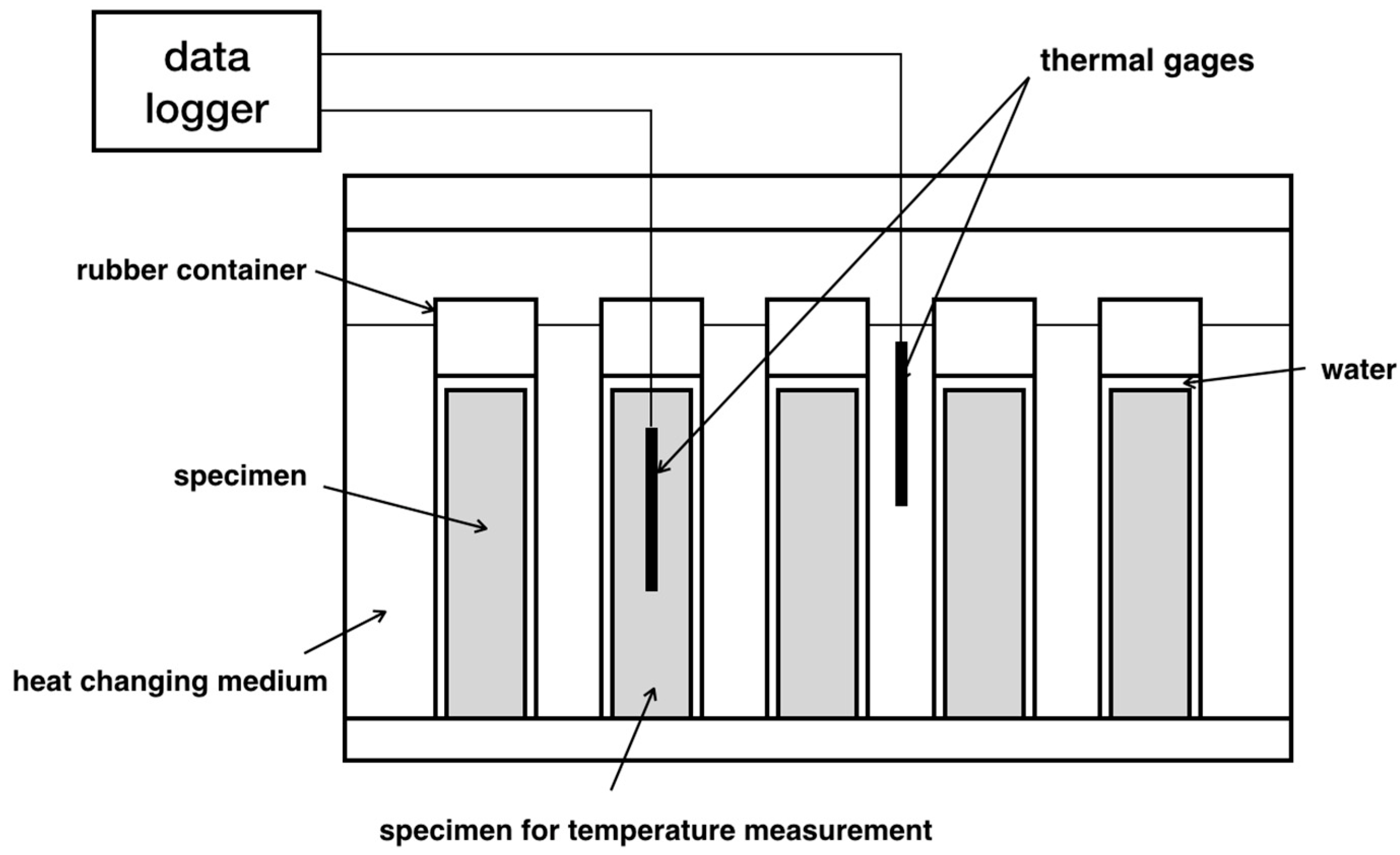
2.1. Test Methods
2.2. Test Variables
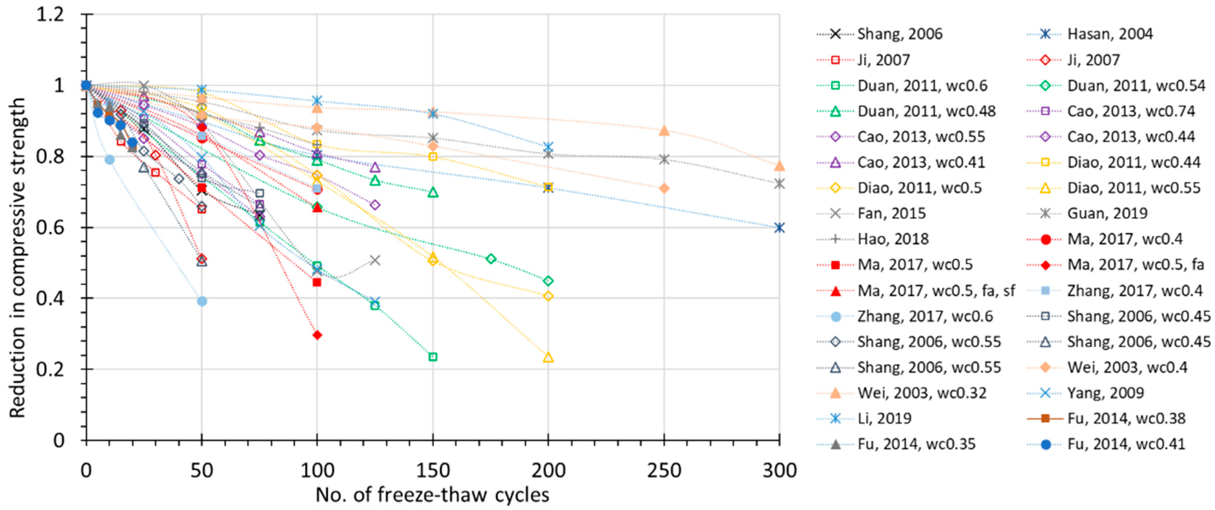
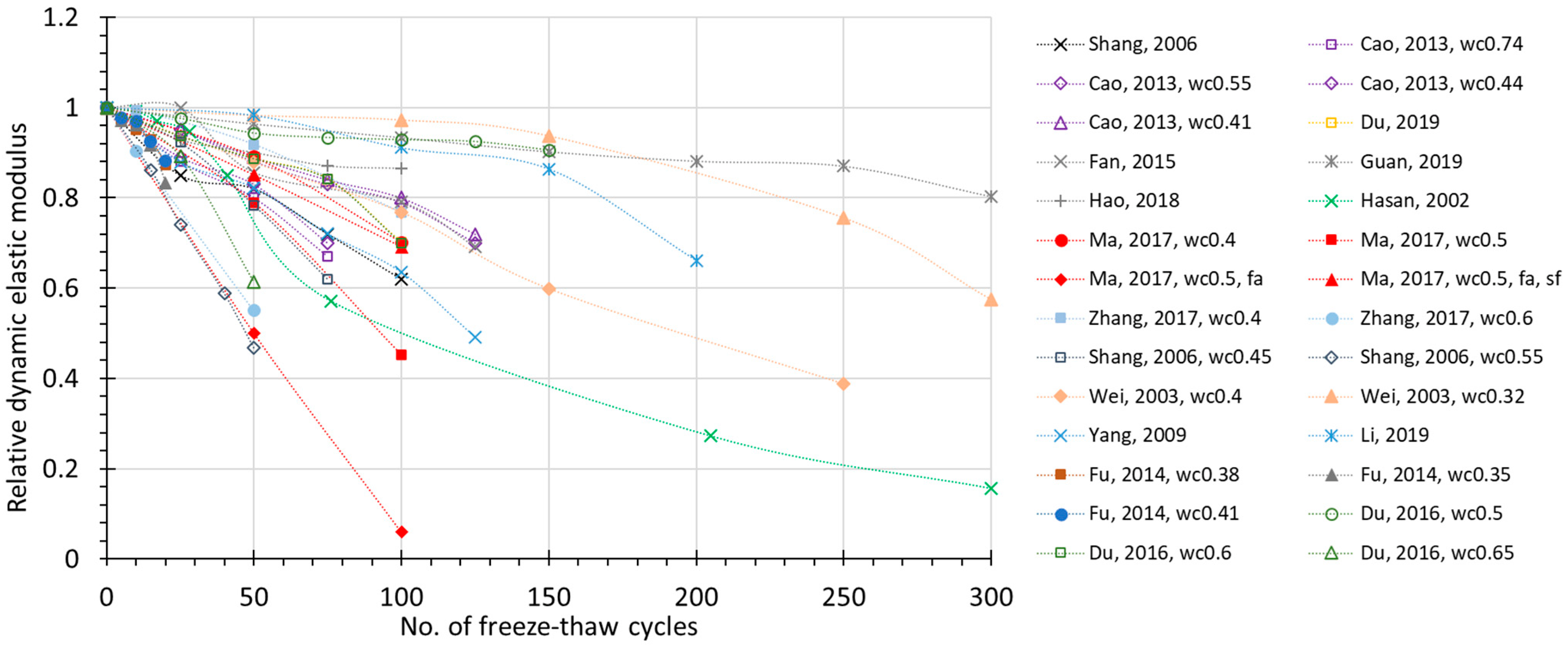
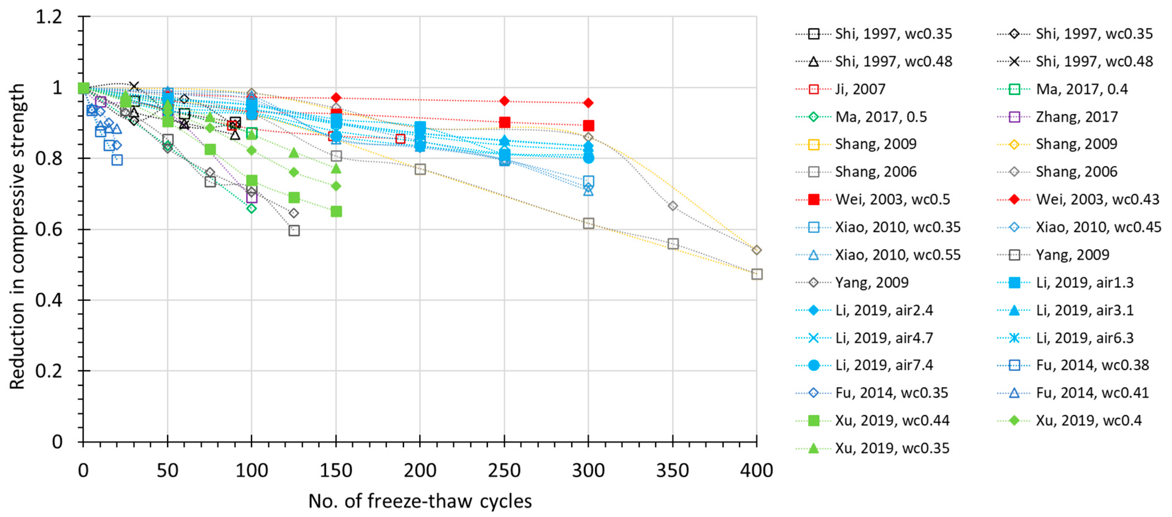
2.3. Test Results
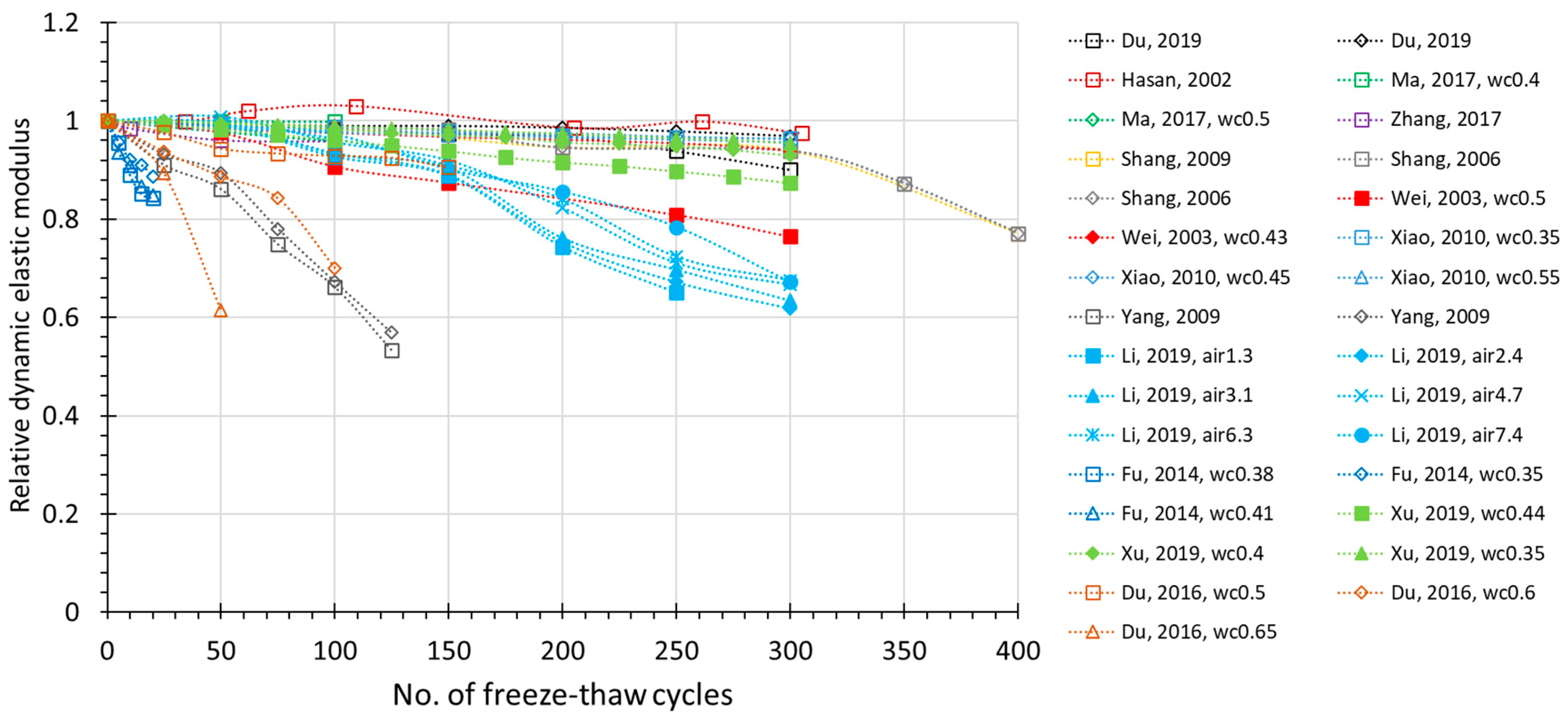
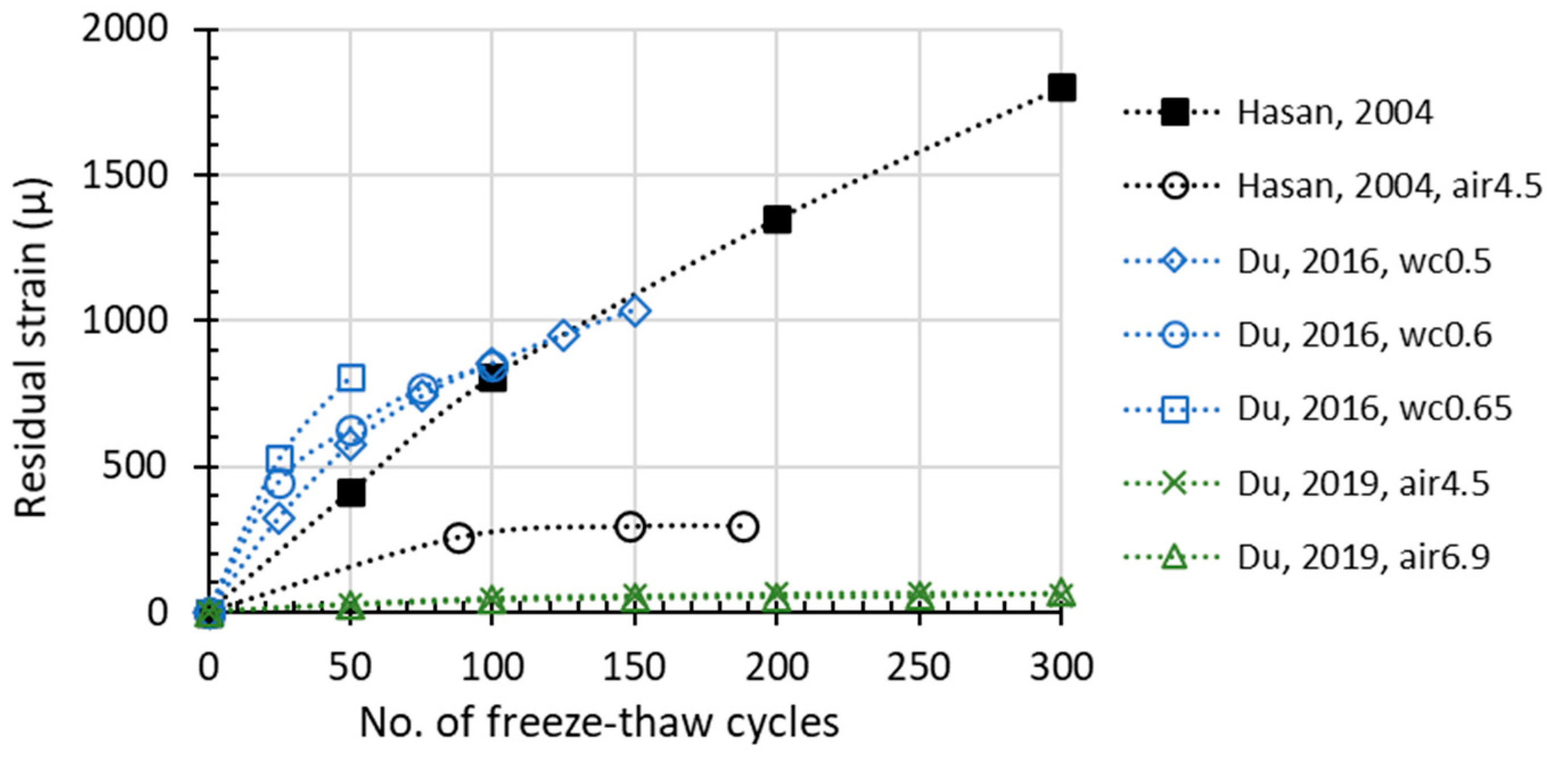
2.3.1. Indexes Change with FTC Number
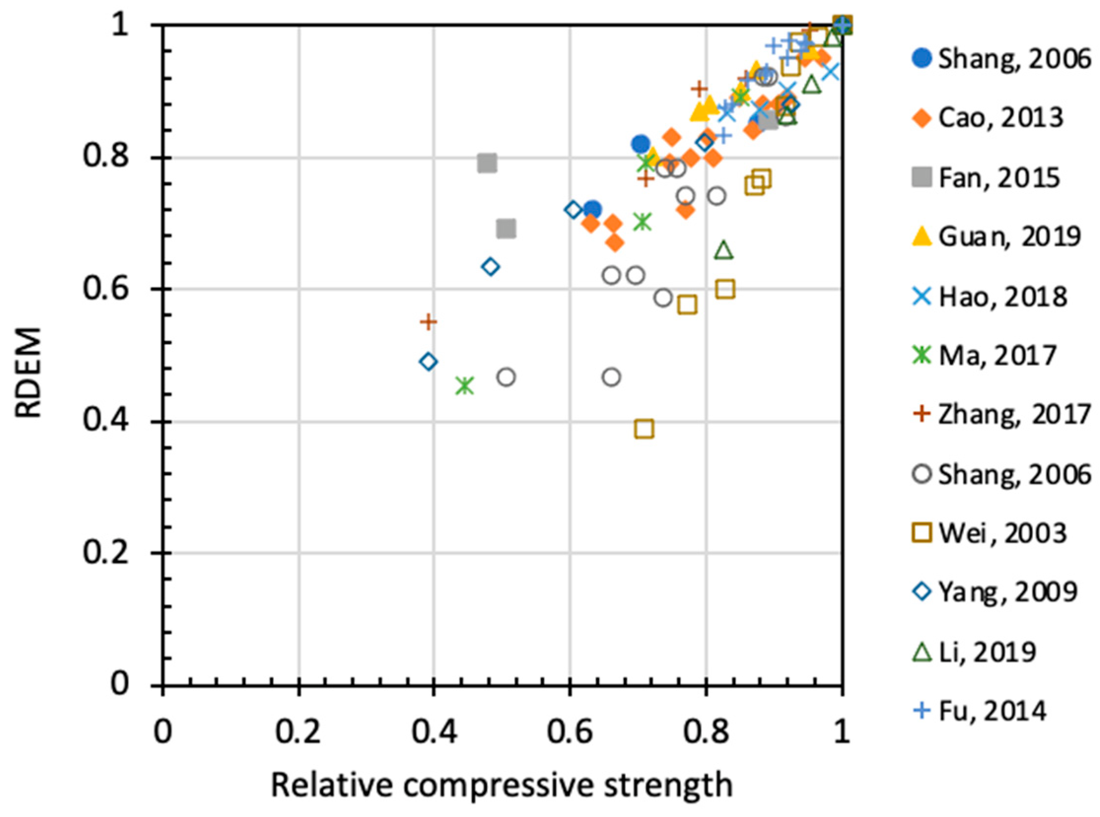
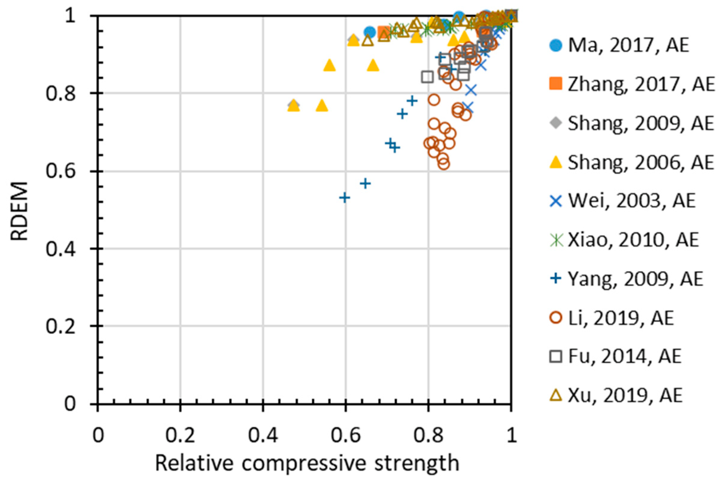
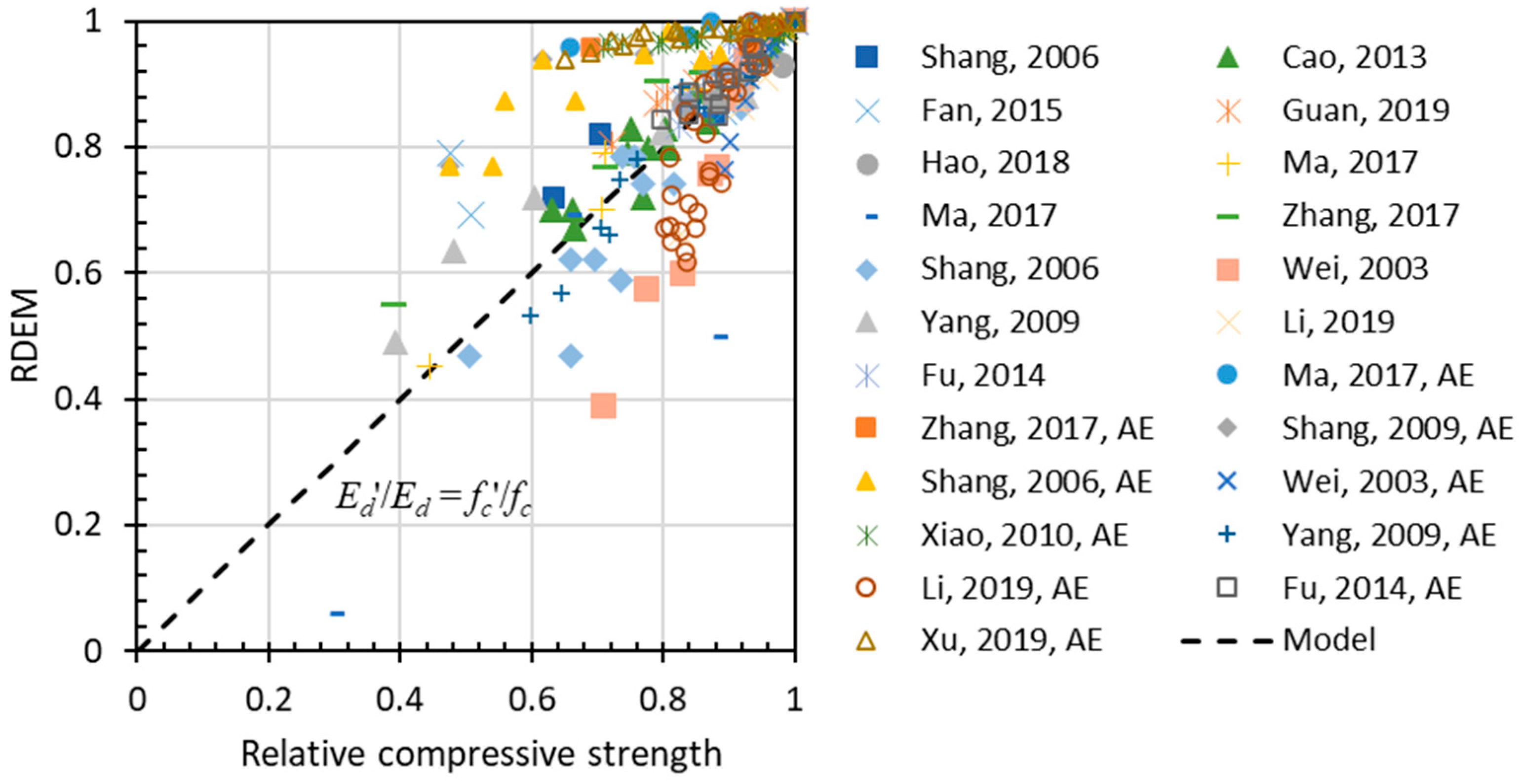
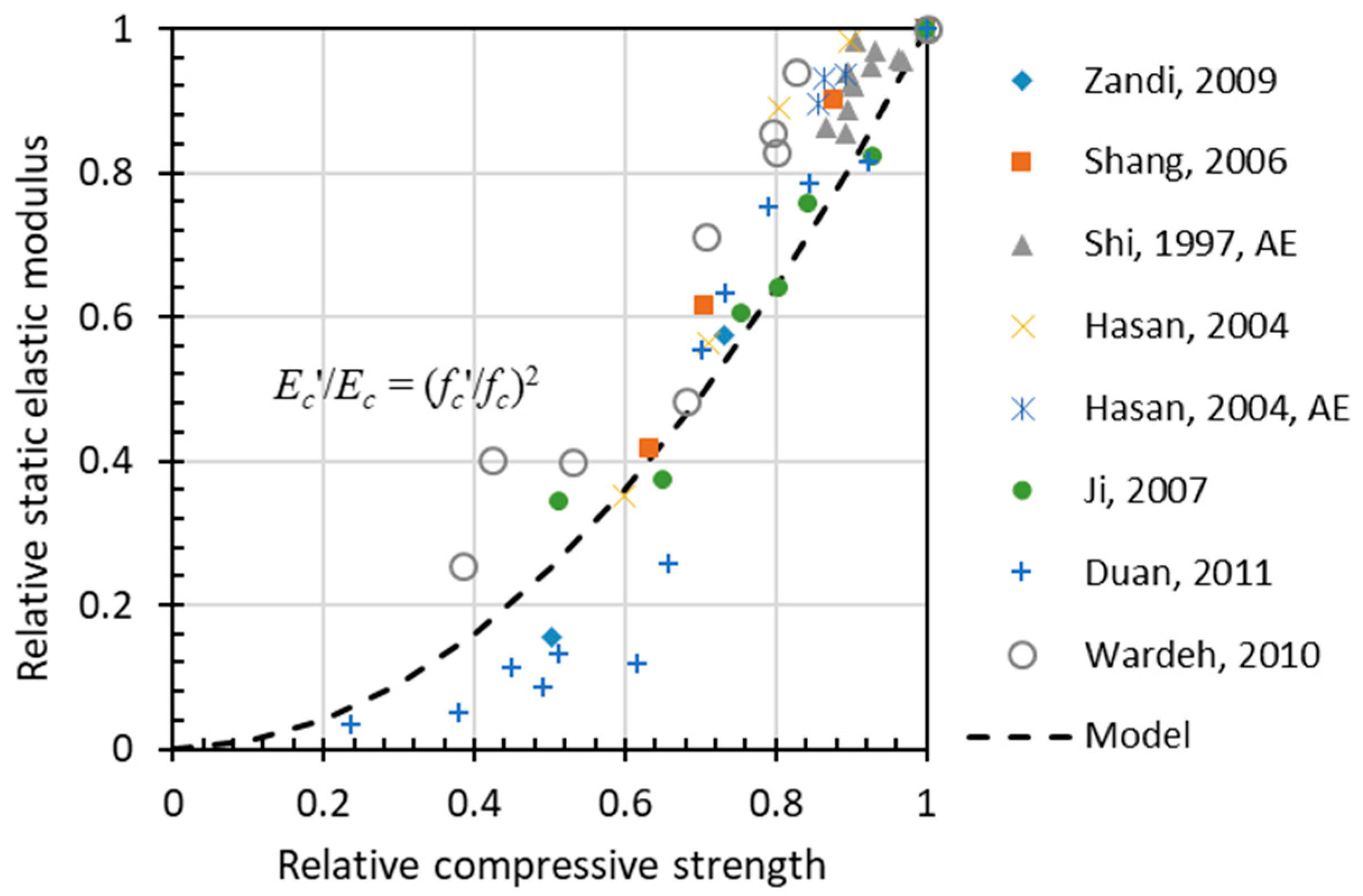
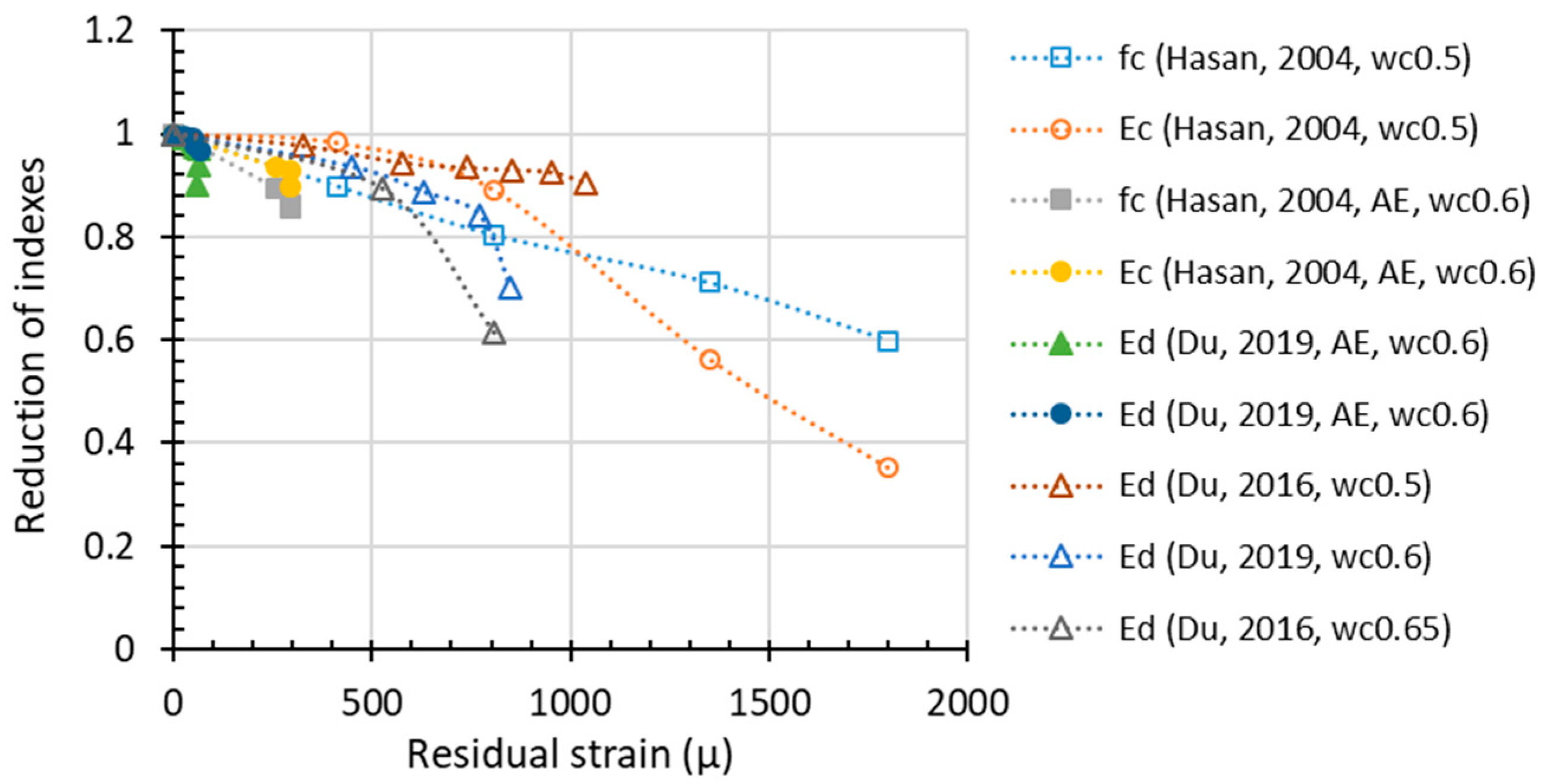
2.3.2. Correlations among Damaged Properties
3. Analysis and Modeling
3.1. Adoptable Models
3.1.1. Linear Model
3.1.2. Exponential Model
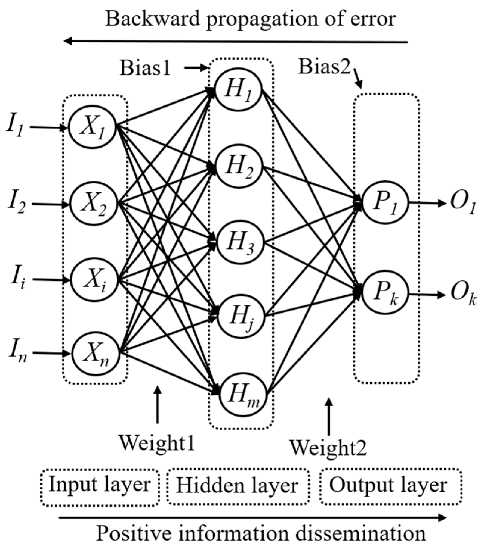
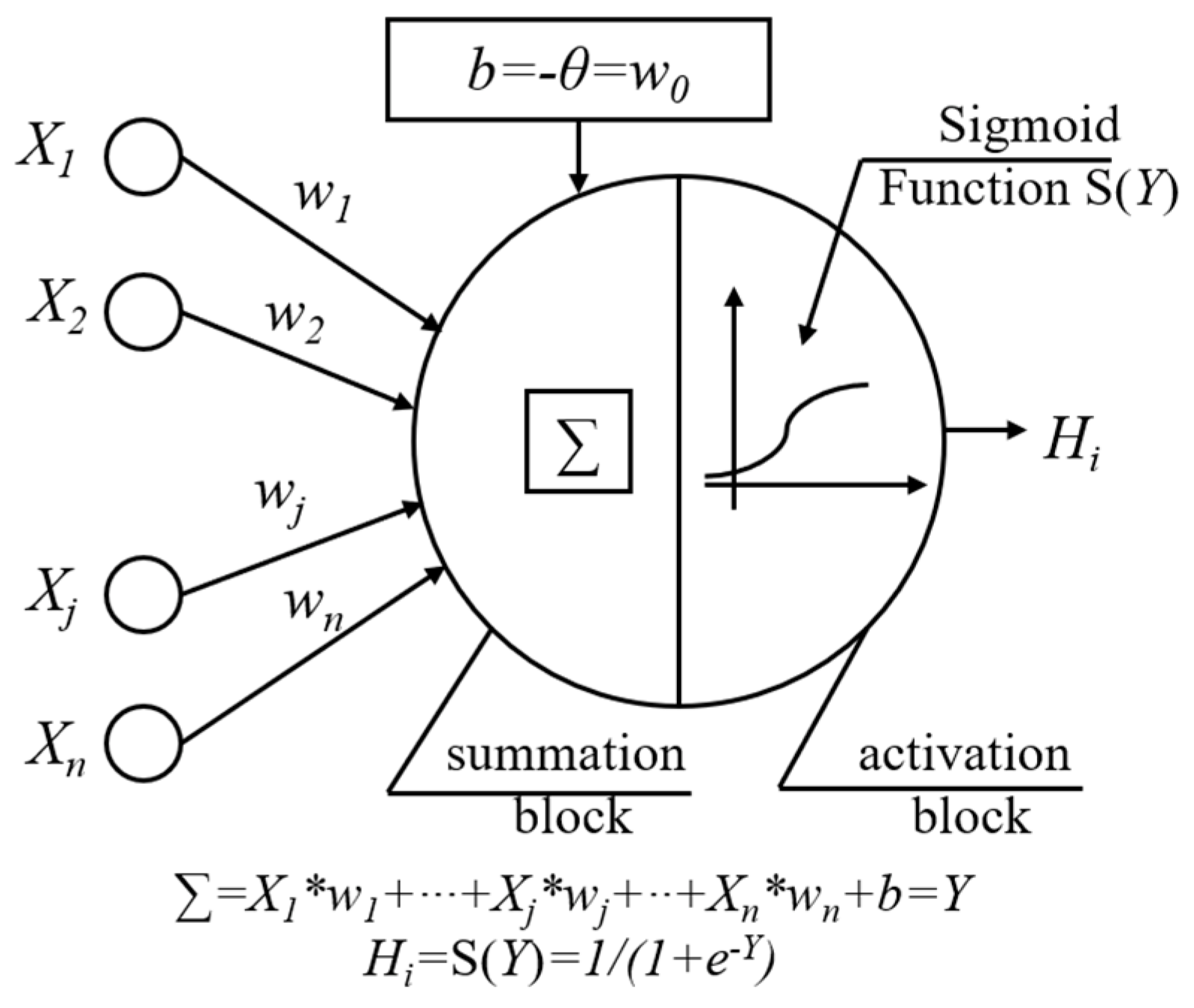
3.1.3. Artificial Neural Network Model
3.2. Regression and Discussion
3.2.1. Data Selection and Pretreatment
3.2.2. Regression Result and Discussion
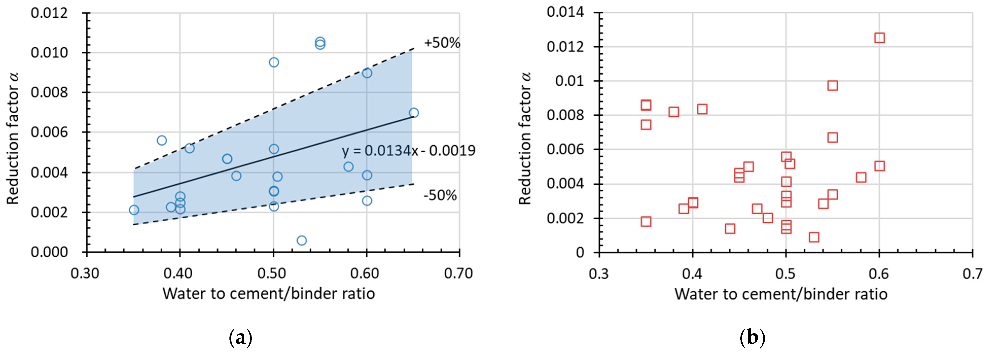
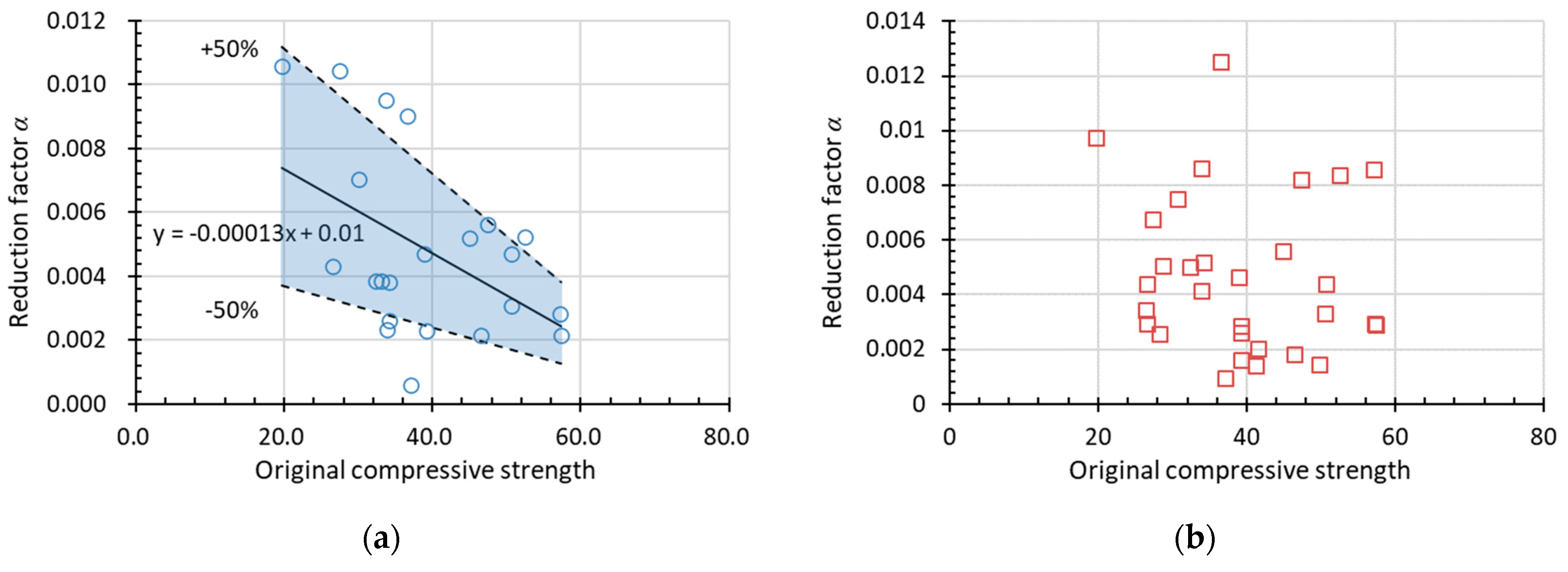
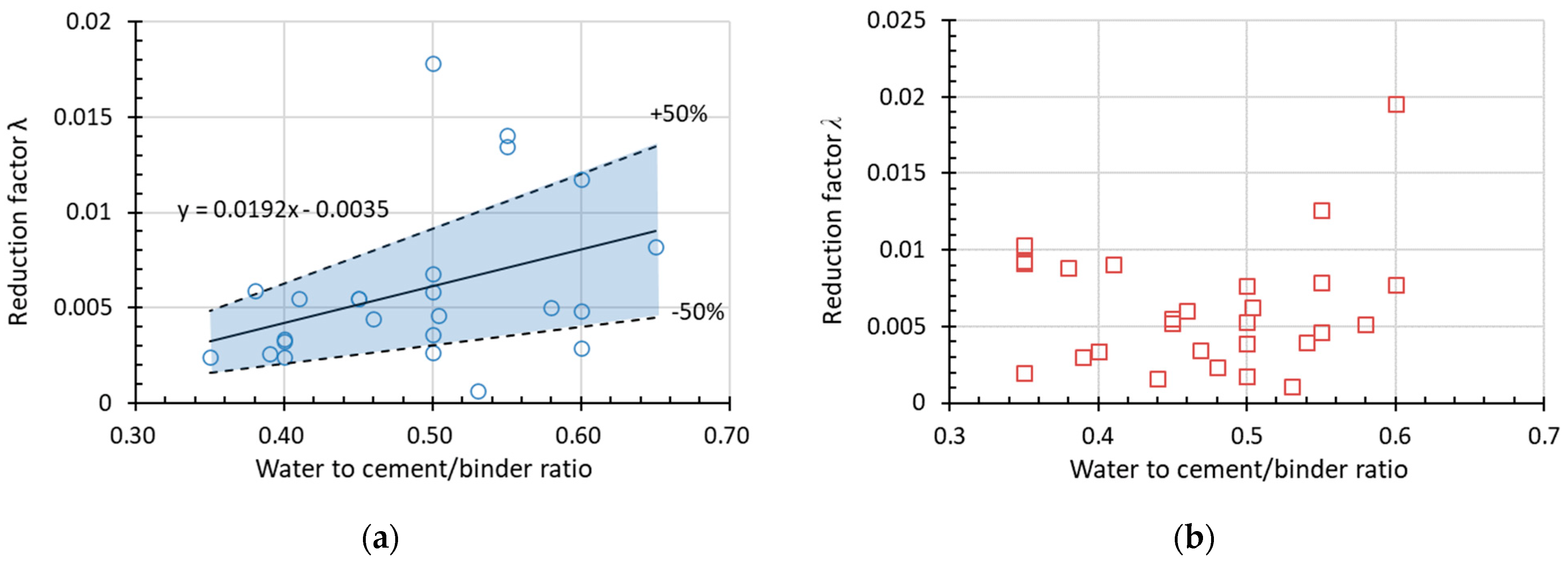
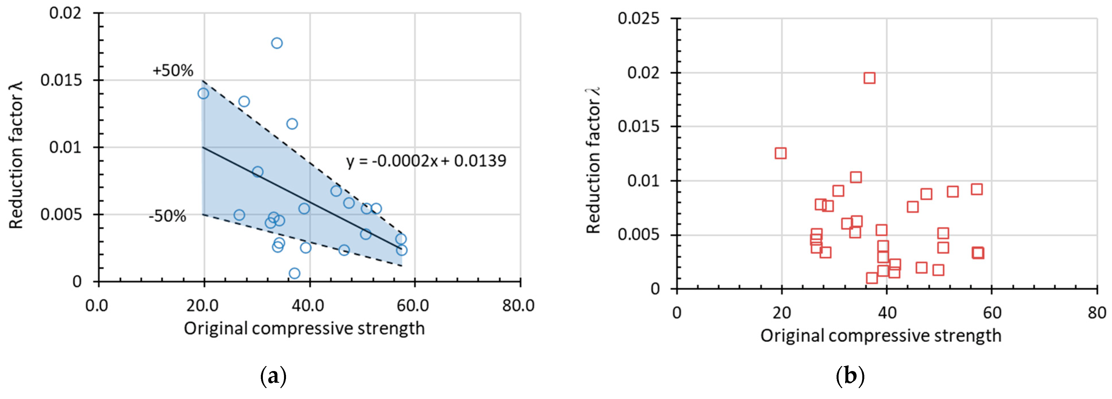
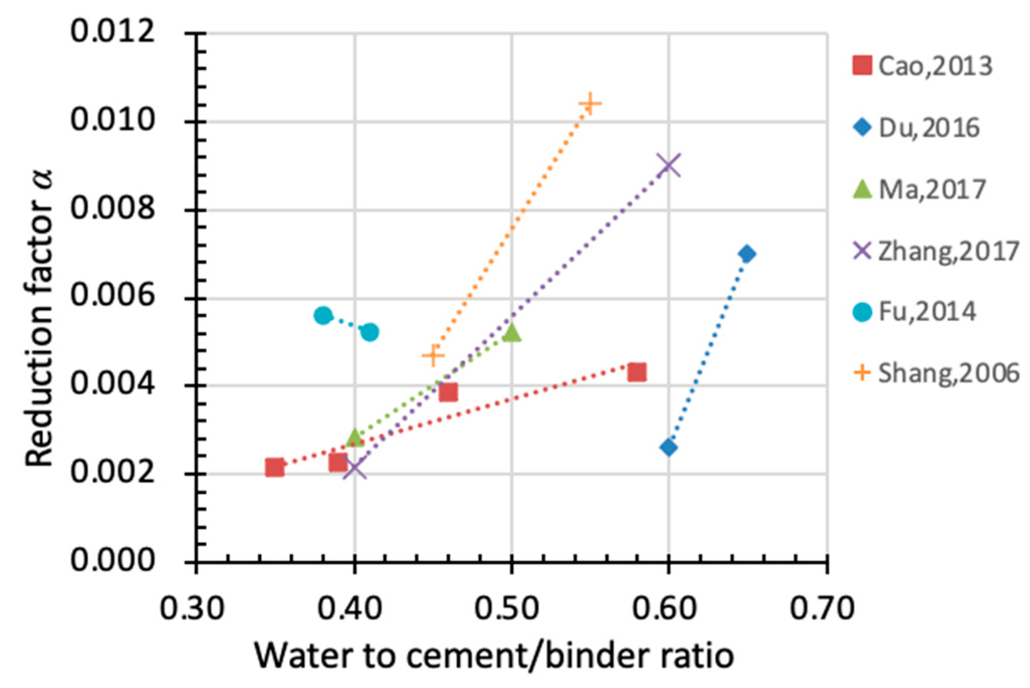
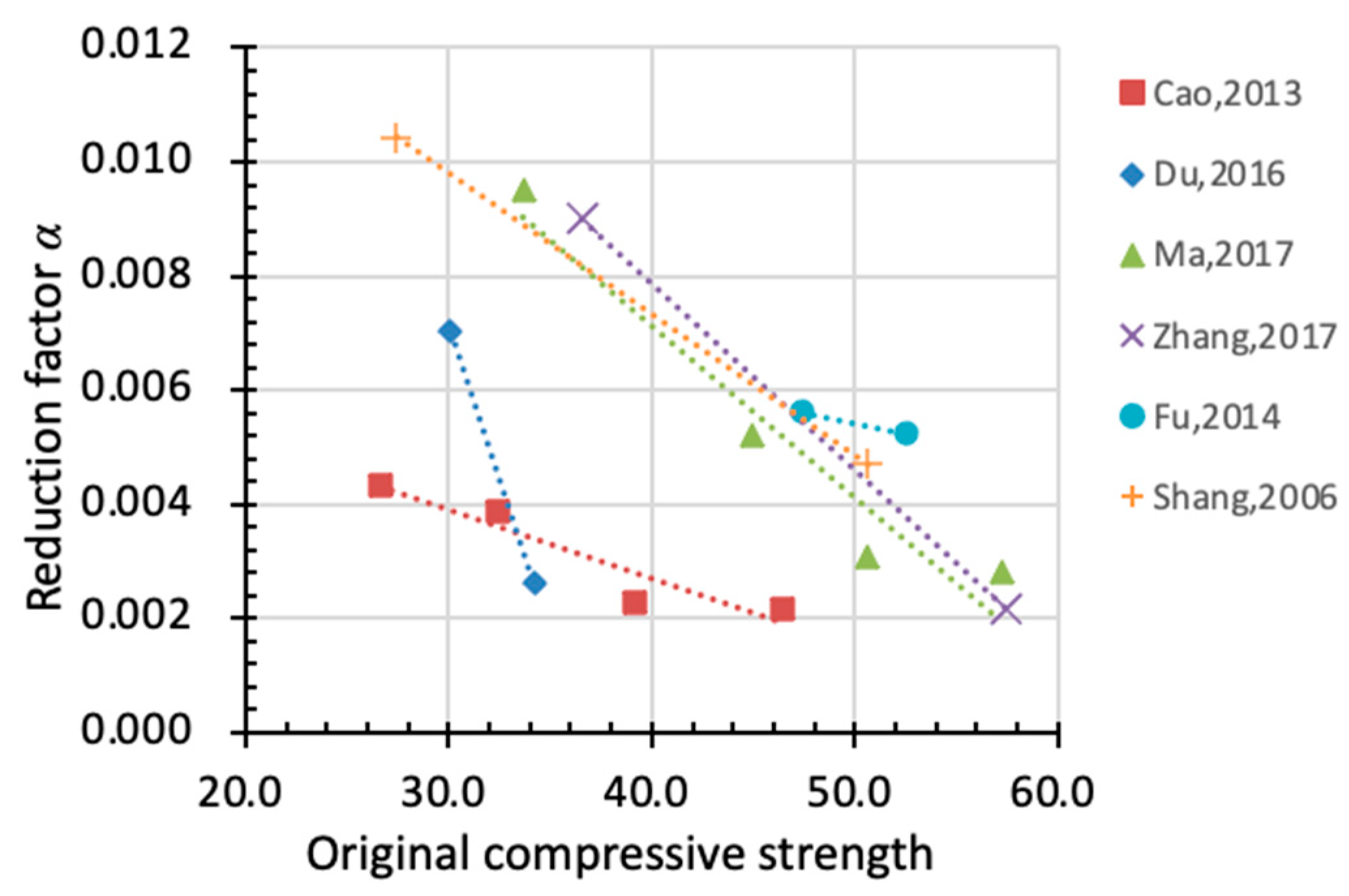
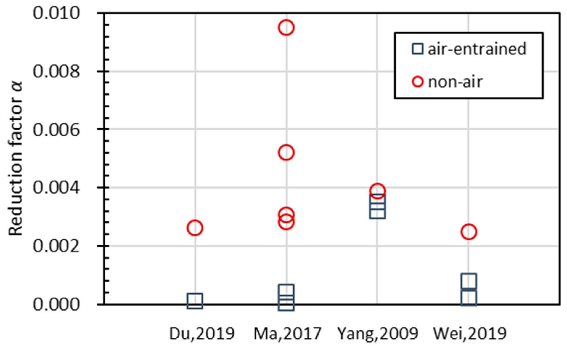
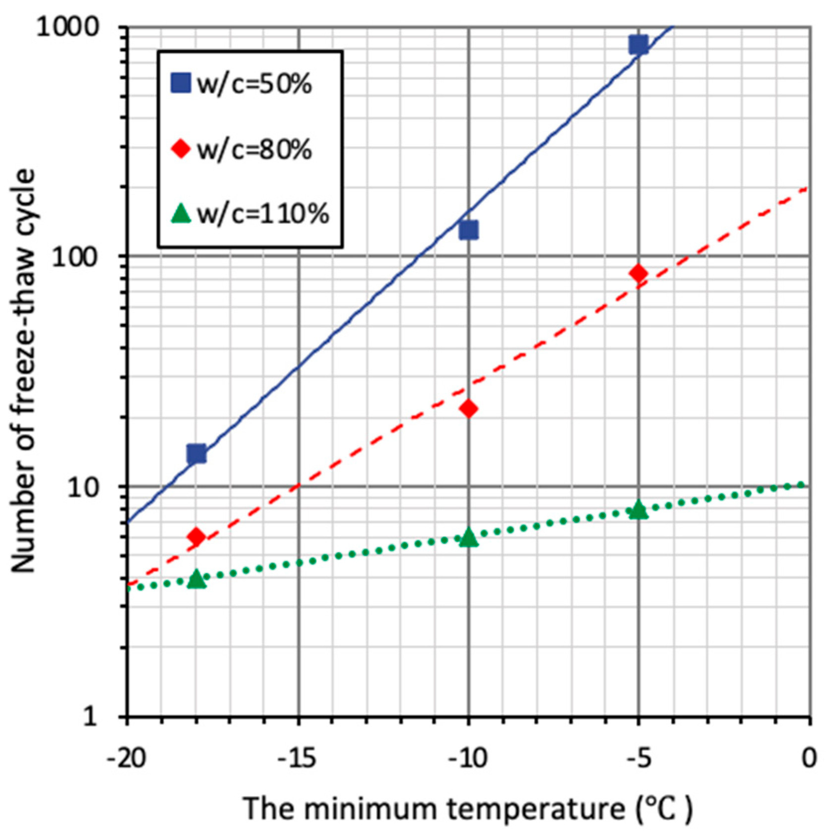
3.2.3. Influencing Factors on Deterioration Speed
3.2.4. Analysis Based on ANN
3.3. Durability Factor
3.4. Further Discussions
4. Conclusions
- (1)
- Experimental conditions and material parameters have significant effects on the behavior of concrete subjected to freezing–thawing tests that are conducted under the guidance of different testing standards. The relationship between damaged indexes and the number of cycles shows a reasonable tendency, where a larger water-to-cement ratio and lower original strength cause faster deterioration with more FT cycles. Yet, a lack of consistency between results from different works is substantial. Correlations among damaged properties were carefully analyzed and stable results can be obtained.
- (2)
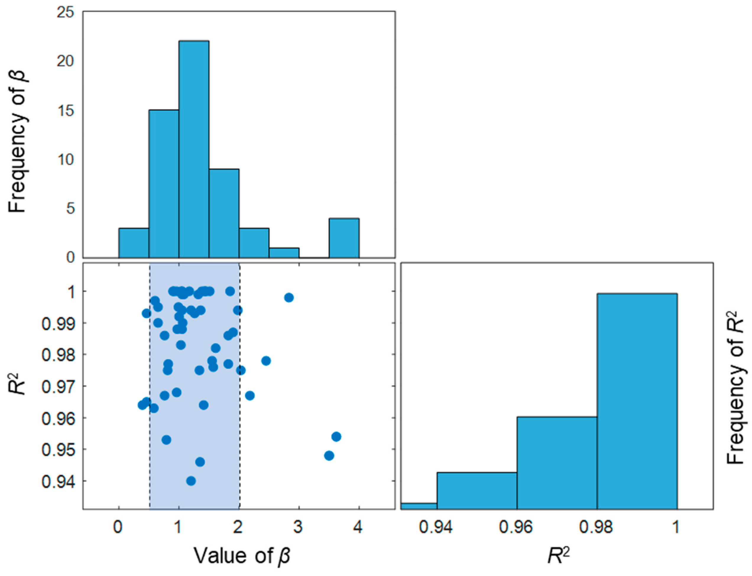
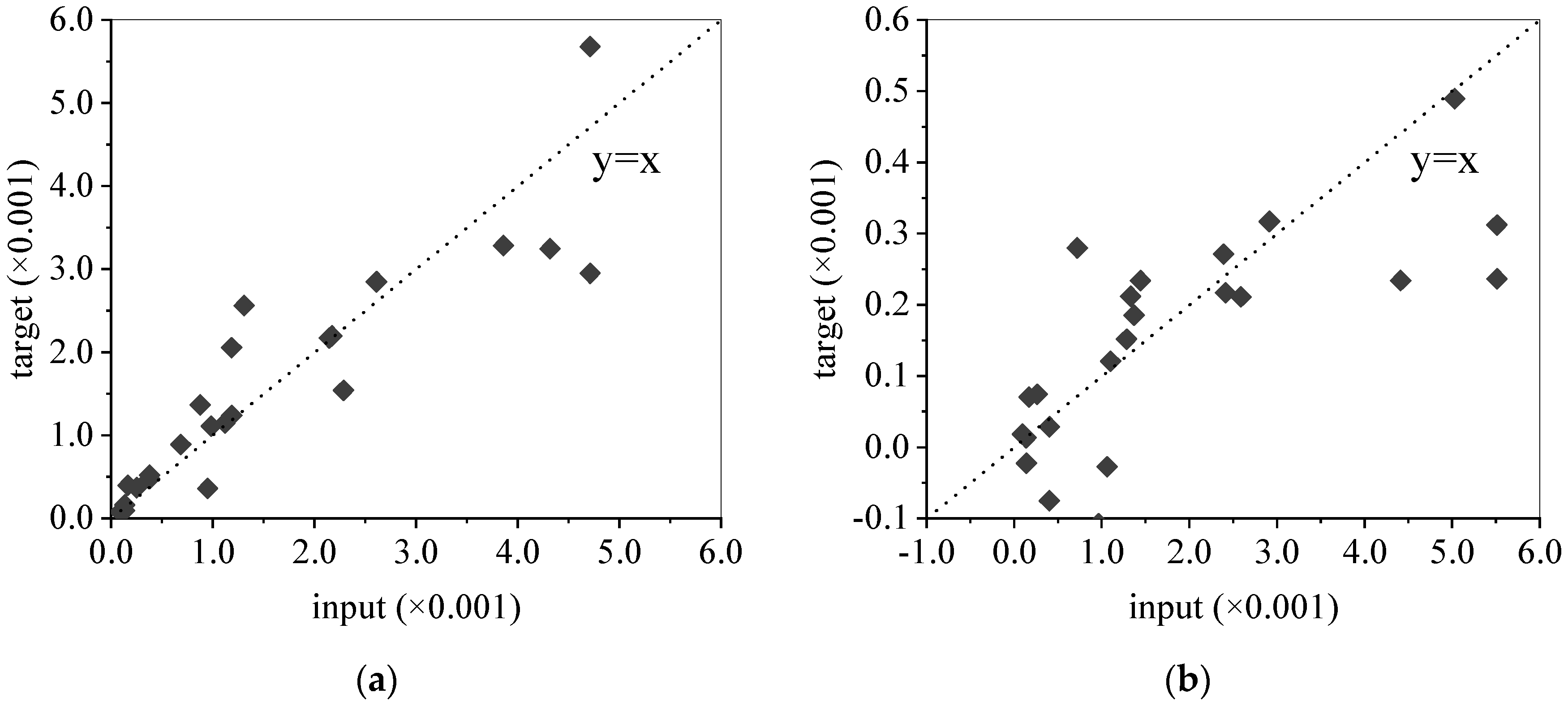
- Two prediction models of RDEM degradation under the effect of frost damage were proposed, namely, the linear model and the exponential model. Briefly, ±50% accuracy can be achieved after proper selection and pretreatment with data. This further proves the scattering nature of the experimental data and the importance of applying the statistical analysis. Moreover, a model based on an Artificial Neural Network was also suggested in this paper; although it can give nice predicting results, the authors do not recommend this way due to a lack of physical and logical meaning.
- (3)
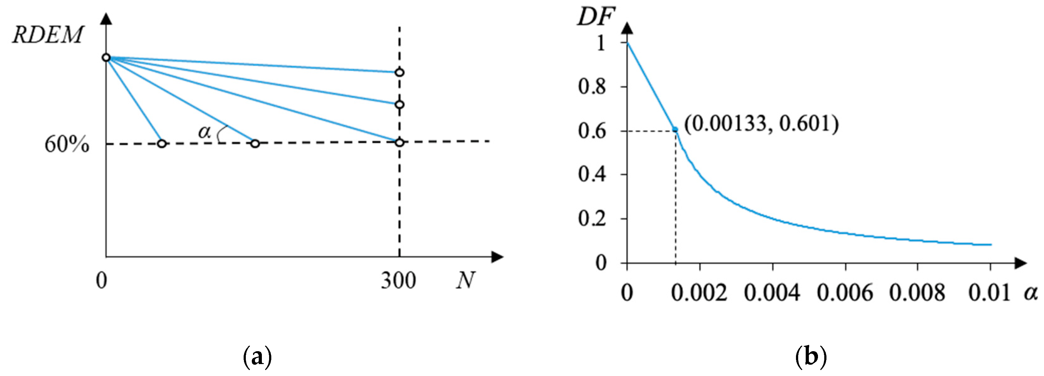
- To quantify the frost resistance ability of different materials, the durability factor (DF) was discussed in the paper. The correlation between the DF and the reduction factor α serves as an alternative index to evaluate the resistivity of materials. The DF can be regarded as a material characteristic which has the physical meaning of frost resistance of the concrete. This will help to evaluate the experiments that do not follow the standard testing requirements. Besides, this factor of the DF can be easily used and understood by the engineering application to judge the frost resistance, even though the standard test is not exactly followed. Further research will be needed to figure out the response of basic evaluation indexes under various experimental conditions.
- (4)
- For the practical evaluation of frost-damaged behaviors, the overall evaluation can be achieved after measuring one or two indexes (residual strain, RDEM, or compressive strength), while for the time-dependent frost damage progress, it seems that the scattering of FTC experiments is even more dominant than the logic rules of the frost mechanism. Thus, it may be more reliable to adopt theoretical and numerical models to obtain the general predicting formulae, which will be conducted in the future.
Author Contributions
Funding
Institutional Review Board Statement
Informed Consent Statement
Data Availability Statement
Conflicts of Interest
Appendix A

| ID | w/c | fc | Air Void [%] | Tmin | y = 1 − αNβ | y = exp(−λN) | DF 1 | DF 2 | Ref. | |||||
|---|---|---|---|---|---|---|---|---|---|---|---|---|---|---|
| α | β | R2 | α (β = 1) | R2 | λ | R2 | ||||||||
| 1 | 0.50 | 34.2 | (non-AE) | −15 | 8.9 × 10⁻³ | 0.81 | 0.97 | 3.8 × 10⁻³ | 0.96 | 4.6 × 10⁻³ | 0.97 | 0.20 | 0.21 | Shang, 2006 [36] |
| 2 | 0.75 | 26.6 | 3.6 (non-AE) | −17 | 4.4 × 10⁻³ | 1.00 | 0.99 | 4.3 × 10⁻³ | 0.99 | 5.0 × 10⁻³ | 0.99 | - | 0.19 | Cao, 2013 [38] |
| 3 | 0.55 | 32.4 | 3.4 (non-AE) | −17 | 3.4 × 10⁻³ | 1.03 | 0.98 | 3.9 × 10⁻³ | 0.98 | 4.4 × 10⁻³ | 0.98 | - | 0.21 | Cao, 2013 [38] |
| 4 | 0.44 | 39.2 | 2.6 (non-AE) | −17 | 1.7 × 10⁻³ | 1.06 | 0.99 | 2.3 × 10⁻³ | 0.99 | 2.6 × 10⁻³ | 0.98 | - | 0.35 | Cao, 2013 [38] |
| 5 | 0.41 | 46.5 | 3 (non-AE) | −17 | 1.7 × 10⁻³ | 1.05 | 0.99 | 2.1 × 10⁻³ | 0.99 | 2.4 × 10⁻³ | 0.99 | - | 0.37 | Cao, 2013 [38] |
| 6 | 0.60 | 34.2 | 2.8 (non-AE) | −20 | 4.3 × 10⁻⁴ | 1.41 | 0.96 | 2.6 × 10⁻³ | 0.94 | 2.9 × 10⁻³ | 0.92 | - | 0.31 | Du, 2019 [52] |
| 7 | 0.60 | 27.4 | 4.5 (AE) | −20 | 3.7 × 10⁻⁷ | 2.18 | 0.97 | 2.5 × 10⁻⁴ | 0.84 | 2.6 × 10⁻⁴ | 0.83 | 0.90 | 0.92 | Du, 2019 [52] |
| 8 | 0.60 | 22.8 | 6.9 (AE) | −20 | 1.3 × 10⁻⁵ | 1.35 | 0.95 | 8.9 × 10⁻⁵ | 0.92 | 9.0 × 10⁻⁵ | 0.92 | 0.97 | 0.97 | Du, 2019 [52] |
| 9 | 0.50 | 33.9 | (non-AE) | −20 | 9.0 × 10⁻⁴ | 1.20 | 0.94 | 2.3 × 10⁻³ | 0.93 | 2.6 × 10⁻³ | 0.92 | - | 0.35 | Fan, 2015 [53] |
| 10 | 0.53 | 37.1 | (non-AE) | −18 | 7.6 × 10⁻⁴ | 0.96 | 0.97 | 6.1 × 10⁻⁴ | 0.97 | 6.6 × 10⁻⁴ | 0.97 | 0.80 | 0.82 | Guan, 2019 [54] |
| 11 | 0.50 | 39.3 | (non-AE) | −18 | 1.6 × 10⁻² | 0.46 | 0.99 | 1.6 × 10⁻³ | 0.82 | 1.7 × 10⁻³ | 0.85 | - | 0.50 | Hao, 2018 [55] |
| 12 | 0.50 | - | (non-AE) | −17.8 | 1.0 × 10⁻² | 0.79 | 0.95 | 3.1 × 10⁻³ | 0.93 | 5.8 × 10⁻³ | 0.97 | 0.14 | 0.26 | Hasan, 2002 [51] |
| 13 | 0.40 | 57.2 | (non-AE) | −17 | 3.7 × 10⁻⁴ | 1.45 | 1.00 | 2.8 × 10⁻³ | 0.97 | 3.2 × 10⁻³ | 0.95 | - | 0.28 | Ma, 2017 [50] |
| 14 | 0.50 | 44.9 | (non-AE) | −17 | 9.4 × 10⁻⁴ | 1.38 | 1.00 | 5.2 × 10⁻³ | 0.98 | 6.8 × 10⁻³ | 0.94 | 0.16 | 0.15 | Ma, 2017 [50] |
| 15 | 0.40 | 43.6 | (AE) | −17 | 8.2 × 10⁻⁶ | 1.17 | 1.00 | 1.8 × 10⁻⁵ | 1.00 | 1.8 × 10⁻⁵ | 1.00 | - | 0.99 | Ma, 2017 [50] |
| 16 | 0.50 | 37.4 | (AE) | −17 | 6.6 × 10⁻⁴ | 0.90 | 1.00 | 4.2 × 10⁻⁴ | 1.00 | 4.2 × 10⁻⁴ | 1.00 | - | 0.88 | Ma, 2017 [50] |
| 17 | 0.50 | 33.7 | (non-AE) | −17 | 1.4 × 10⁻² | 0.91 | 1.00 | 9.5 × 10⁻³ | 1.00 | 1.8 × 10⁻² | 0.96 | 0.08 | 0.08 | Ma, 2017 [50] |
| 18 | 0.50 | 50.6 | (non-AE) | −17 | 2.5 × 10⁻³ | 1.05 | 1.00 | 3.1 × 10⁻³ | 1.00 | 3.6 × 10⁻³ | 0.99 | - | 0.26 | Ma, 2017 [50] |
| 19 | 0.40 | 57.4 | 1.4 (non-AE) | −15 | 2.2 × 10⁻⁴ | 1.51 | 1.00 | 2.2 × 10⁻³ | 0.97 | 2.4 × 10⁻³ | 0.95 | - | 0.37 | Zhang, 2017 [49] |
| 20 | 0.60 | 36.6 | 2.1 (non-AE) | −15 | 1.1 × 10⁻² | 0.96 | 1.00 | 9.0 × 10⁻³ | 1.00 | 1.2 × 10⁻² | 1.00 | 0.09 | 0.09 | Zhang, 2017 [49] |
| 21 | 0.60 | 33.5 | 5.2 (AE) | −15 | 7.3 × 10⁻³ | 0.39 | 0.96 | 4.9 × 10⁻⁴ | 0.69 | 5.1 × 10⁻⁴ | 0.70 | - | 0.85 | Zhang, 2017 [49] |
| 22 | 0.40 | 34.2 | (AE) | −15 | 1.8 × 10⁻¹⁰ | 3.50 | 0.95 | 4.1 × 10⁻⁴ | 0.71 | 4.3 × 10⁻⁴ | 0.70 | 0.94 | 0.88 | Shang, 2009 [48] |
| 23 | 0.40 | 26.3 | (AE) | −15 | 1.8 × 10⁻¹⁰ | 3.50 | 0.95 | 4.1 × 10⁻⁴ | 0.71 | 4.3 × 10⁻⁴ | 0.70 | 0.94 | 0.88 | Shang, 2009 [48] |
| 24 | 0.45 | 50.7 | 0.9 (non-AE) | −18 | 8.0 × 10⁻⁴ | 1.43 | 1.00 | 4.7 × 10⁻³ | 0.97 | 5.5 × 10⁻³ | 0.94 | 0.15 | 0.17 | Shang, 2006 [46] |
| 25 | 0.55 | 27.4 | 1.9 (non-AE) | −18 | 7.7 × 10⁻³ | 1.08 | 1.00 | 1.0 × 10⁻² | 1.00 | 1.3 × 10⁻² | 0.97 | 0.08 | 0.08 | Shang, 2006 [46] |
| 26 | 0.45 | 38.9 | 0.9 (non-AE) | −18 | 8.0 × 10⁻⁴ | 1.43 | 1.00 | 4.7 × 10⁻³ | 0.97 | 5.5 × 10⁻³ | 0.94 | 0.15 | 0.17 | Shang, 2006 [46] |
| 27 | 0.55 | 19.7 | 1.9 (non-AE) | −18 | 9.2 × 10⁻³ | 1.04 | 1.00 | 1.1 × 10⁻² | 1.00 | 1.4 × 10⁻² | 0.98 | 0.08 | 0.08 | Shang, 2006 [46] |
| 28 | 0.40 | 34.2 | 5.5–6.5 (AE) | −18 | 8.4 × 10⁻¹¹ | 3.62 | 0.95 | 3.8 × 10⁻⁴ | 0.73 | 4.0 × 10⁻⁴ | 0.72 | 0.94 | 0.89 | Shang, 2006 [46] |
| 29 | 0.40 | 26.3 | 5.5–6.5 (AE) | −18 | 8.4 × 10⁻¹¹ | 3.62 | 0.95 | 3.8 × 10⁻⁴ | 0.73 | 4.0 × 10⁻⁴ | 0.72 | 0.94 | 0.89 | Shang, 2006 [46] |
| 30 | 0.40 | - | (non-AE) | −15~−20 | 2.6 × 10⁻³ | 0.99 | 0.99 | 2.5 × 10⁻³ | 0.99 | 3.4 × 10⁻³ | 0.97 | 0.3 | 0.32 | Wei, 2003 [45] |
| 31 | 0.32 | - | (non-AE) | −15~−20 | 4.2 × 10⁻⁸ | 2.83 | 1.00 | 1.1 × 10⁻³ | 0.80 | 1.2 × 10⁻³ | 0.76 | 0.58 | 0.68 | Wei, 2003 [45] |
| 32 | 0.50 | - | (AE) | −15~−20 | 9.4 × 10⁻⁴ | 0.97 | 0.99 | 7.9 × 10⁻⁴ | 0.99 | 8.8 × 10⁻⁴ | 0.99 | 0.76 | 0.76 | Wei, 2003 [45] |
| 33 | 0.43 | - | (AE) | −15~−20 | 7.4 × 10⁻⁴ | 0.76 | 0.99 | 2.0 × 10⁻⁴ | 0.96 | 2.1 × 10⁻⁴ | 0.96 | 0.94 | 0.94 | Wei, 2003 [45] |
| 34 | 0.35 | 61.8 | 3.7 (AE) | −18 | 3.5 × 10⁻⁴ | 0.82 | 0.98 | 1.3 × 10⁻⁴ | 0.96 | 1.3 × 10⁻⁴ | 0.96 | 0.96 | 0.96 | Xiao, 2010 [44] |
| 35 | 0.45 | 49.7 | 4.4 (AE) | −18 | 2.5 × 10⁻³ | 0.46 | 0.97 | 1.3 × 10⁻⁴ | 0.76 | 1.4 × 10⁻⁴ | 0.76 | 0.96 | 0.96 | Xiao, 2010 [44] |
| 36 | 0.55 | 32.1 | 4.5 (AE) | −18 | 1.5 × 10⁻³ | 0.60 | 1.00 | 1.6 × 10⁻⁴ | 0.89 | 1.7 × 10⁻⁴ | 0.90 | 0.95 | 0.95 | Xiao, 2010 [44] |
| 37 | 0.60 | 33.1 | (non-AE) | −16 | 3.0 × 10⁻³ | 1.05 | 0.99 | 3.9 × 10⁻³ | 0.99 | 4.8 × 10⁻³ | 0.97 | 0.21 | 0.21 | Yang, 2009 [43] |
| 38 | 0.60 | 31.1 | (AE) | −16 | 1.4 × 10⁻³ | 1.20 | 0.99 | 3.5 × 10⁻³ | 0.98 | 4.2 × 10⁻³ | 0.96 | 0.22 | 0.23 | Yang, 2009 [43] |
| 39 | 0.60 | 30.6 | (AE) | −16 | 6.2 × 10⁻⁴ | 1.36 | 0.99 | 3.2 × 10⁻³ | 0.97 | 3.8 × 10⁻³ | 0.94 | 0.24 | 0.25 | Yang, 2009 [43] |
| 40 | 0.45 | 38.6 | 0.7 (non-AE) | −18 | 7.5 × 10⁻⁷ | 2.45 | 0.98 | 1.3 × 10⁻³ | 0.82 | 1.4 × 10⁻³ | 0.78 | - | 0.61 | Li, 2019 [42] |
| 41 | 0.45 | 37.2 | 1.3 (AE) | −18 | 9.8 × 10⁻⁶ | 1.90 | 0.99 | 1.2 × 10⁻³ | 0.88 | 1.3 × 10⁻³ | 0.84 | - | 0.64 | Li, 2019 [42] |
| 42 | 0.45 | 35.8 | 2.4 (AE) | −18 | 5.8 × 10⁻⁵ | 1.55 | 0.98 | 1.2 × 10⁻³ | 0.92 | 1.4 × 10⁻³ | 0.89 | 0.62 | 0.64 | Li, 2019 [42] |
| 43 | 0.45 | 33.1 | 3.1 (AE) | −18 | 5.0 × 10⁻⁵ | 1.57 | 0.98 | 1.1 × 10⁻³ | 0.91 | 1.3 × 10⁻³ | 0.88 | 0.63 | 0.66 | Li, 2019 [42] |
| 44 | 0.45 | 30.3 | 4.7 (AE) | −18 | 1.1 × 10⁻⁵ | 1.82 | 0.98 | 9.8 × 10⁻⁴ | 0.87 | 1.1 × 10⁻³ | 0.84 | 0.67 | 0.71 | Li, 2019 [42] |
| 45 | 0.45 | 26.8 | 6.3 (AE) | −18 | 1.1 × 10⁻⁵ | 1.82 | 0.99 | 9.5 × 10⁻⁴ | 0.88 | 1.1 × 10⁻³ | 0.85 | 0.68 | 0.71 | Li, 2019 [42] |
| 46 | 0.45 | 21.2 | 7.4 (AE) | −18 | 4.1 × 10⁻⁶ | 1.98 | 0.99 | 8.7 × 10⁻⁴ | 0.87 | 9.6 × 10⁻⁴ | 0.84 | 0.67 | 0.74 | Li, 2019 [42] |
| 47 | 0.38 | 47.4 | (non-AE) | −17 | 2.2 × 10⁻³ | 1.34 | 0.97 | 5.6 × 10⁻³ | 0.95 | 5.9 × 10⁻³ | 0.95 | - | 0.14 | Fu, 2014 [41] |
| 48 | 0.35 | 57.1 | (non-AE) | −17 | 3.7 × 10⁻⁴ | 2.03 | 0.98 | 6.8 × 10⁻³ | 0.87 | 7.1 × 10⁻³ | 0.85 | - | 0.12 | Fu, 2014 [41] |
| 49 | 0.41 | 52.5 | (non-AE) | −17 | 9.5 × 10⁻⁴ | 1.61 | 0.98 | 5.2 × 10⁻³ | 0.93 | 5.5 × 10⁻³ | 0.92 | - | 0.15 | Fu, 2014 [41] |
| 50 | 0.38 | 14.6 | (AE) | −17 | 1.7 × 10⁻² | 0.76 | 0.97 | 8.9 × 10⁻³ | 0.94 | 9.7 × 10⁻³ | 0.95 | - | 0.09 | Fu, 2014 [41] |
| 51 | 0.35 | 25.3 | (AE) | −17 | 1.6 × 10⁻² | 0.65 | 0.99 | 6.1 × 10⁻³ | 0.93 | 6.5 × 10⁻³ | 0.94 | - | 0.13 | Fu, 2014 [41] |
| 52 | 0.41 | 16.5 | (AE) | −17 | 2.2 × 10⁻² | 0.65 | 0.99 | 8.4 × 10⁻³ | 0.94 | 9.1 × 10⁻³ | 0.95 | - | 0.10 | Fu, 2014 [41] |
| 53 | 0.44 | 42.2 | (AE) | −16 | 3.1 × 10⁻⁴ | 1.05 | 1.00 | 4.1 × 10⁻⁴ | 1.00 | 4.3 × 10⁻⁴ | 1.00 | 0.87 | 0.88 | Xu, 2019 [40] |
| 54 | 0.40 | 51.6 | (AE) | −16 | 5.2 × 10⁻⁵ | 1.26 | 0.99 | 2.1 × 10⁻⁴ | 0.97 | 2.2 × 10⁻⁴ | 0.97 | 0.93 | 0.94 | Xu, 2019 [40] |
| 55 | 0.35 | 62.9 | (AE) | −16 | 2.5 × 10⁻⁵ | 1.32 | 1.00 | 1.4 × 10⁻⁴ | 0.97 | 1.4 × 10⁻⁴ | 0.97 | 0.95 | 0.96 | Xu, 2019 [40] |
| 56 | 0.50 | 40.7 | 2.5 (non-AE) | −18 | 4.9 × 10⁻³ | 0.58 | 0.96 | 6.8 × 10⁻⁴ | 0.85 | 7.2 × 10⁻⁴ | 0.87 | - | 0.79 | Du, 2016 [57] |
| 57 | 0.65 | 30.1 | 3.2 (non-AE) | −18 | 2.8 × 10⁻⁴ | 1.85 | 1.00 | 7.0 × 10⁻³ | 0.93 | 8.2 × 10⁻³ | 0.89 | - | 0.11 | Du, 2016 [57] |
References
- Setzer, M.J. Micro-ice-lens formation in porous solid. J. Colloid Interface Sci. 2001, 243, 193–201. [Google Scholar] [CrossRef]
- Powers, T.C. A working hypothesis for further studies of frost resistance of concrete. J. Proc. 1945, 41, 245–272. [Google Scholar]
- Koniorczyk, M.; Gawin, D.; Schrefler, B.A. Modeling evolution of frost damage in fully saturated porous materials exposed to variable hygro-thermal conditions. Comput. Methods Appl. Mech. Eng. 2015, 297, 38–61. [Google Scholar] [CrossRef]
- Bazănt, Z.P.; Chern, J.C.; Rosenberg, A.M.; Gaidis, J.M. Mathematical model for freeze-thaw durability of concrete. J. Am. Ceram. Soc. Am. Ceram. Soc. 1988, 71, 776–783. [Google Scholar] [CrossRef]
- Chalangaran, N.; Farzampour, A.; Paslar, N. Nano silica and metakaolin effects on the behavior of concrete containing rubber crumbs. Civil Eng. 2020, 1, 264–274. [Google Scholar] [CrossRef]
- Mansouri, I.; Shahheidari, F.S.; Hashemi, S.M.A.; Farzampour, A. Investigation of steel fiber effects on concrete abrasion resistance. Adv. Concr. Constr. 2020, 9, 367–374. [Google Scholar]
- Chalangaran, N.; Farzampour, A.; Paslar, N.; Fatemi, H. Experimental investigation of sound transmission loss in concrete containing recycled rubber crumbs. Adv. Concr. Constr. 2021, 11, 447–454. [Google Scholar]
- Coussy, O.; Monteiro, P.J. Poroelastic model for concrete exposed to freezing temperatures. Cem. Concr. Res. 2008, 38, 40–48. [Google Scholar] [CrossRef]
- Scherer, G.W.; Valenza, J. Mechanisms of frost damage. Mater. Sci. Concr. 2005, 7, 209–246. [Google Scholar]
- Gong, F.; Sicat, E.; Zhang, D.; Ueda, T. Stress analysis for concrete materials under multiple freeze-thaw cycles. J. Adv. Concr. Technol. 2015, 13, 124–134. [Google Scholar] [CrossRef]
- Zeng, Q.; Fen-Chong, T.; Dangla, P.; Li, K. A study of freezing behavior of cementitious materials by poromechanical approach. Int. J. Solids Struct. 2011, 48, 3267–3273. [Google Scholar] [CrossRef]
- Zeng, Q.; Fen-Chong, T.; Li, K.-F. Elastic behavior of saturated porous materials under undrained freezing. Acta Mech. Sin. 2013, 29, 827–835. [Google Scholar] [CrossRef]
- Sun, Z.; Scherer, G.W. Effect of air voids on salt scaling and internal freezing. Cem. Concr. Res. 2010, 40, 260–270. [Google Scholar] [CrossRef]
- Gong, F.; Jacobsen, S. Modeling of water transport in highly saturated concrete with wet surface during freeze/thaw. Cem. Concr. Res. 2019, 115, 294–307. [Google Scholar] [CrossRef]
- Fagerlund, G. Mechanical damage and fatigue effects associated with freeze-thaw of materials. In Proceedings of International RILEM Workshop of Frost Resistance of Concrete; RILEM Publications SARL: Paris, France, 2002; pp. 117–132. [Google Scholar]
- Jacobsen, S.; Sellevold, E.J.; Matala, S. Frost durability of high strength concrete: Effect of internal cracking on ice formation. Cem. Concr. Res. 1996, 26, 919–931. [Google Scholar] [CrossRef]
- Hasan, M.; Okuyama, H.; Sato, Y.; Ueda, T. Stress-strain model of concrete damaged by freezing and thawing cycles. J. Adv. Concr. Technol. 2004, 2, 89–99. [Google Scholar] [CrossRef]
- Gong, F.; Wang, Y.; Zhang, D.; Ueda, T. Mesoscale simulation of deformation for mortar and concrete under cyclic freezing and thawing stress. J. Adv. Concr. Technol. 2015, 13, 291–304. [Google Scholar] [CrossRef]
- Yang, Z.; Weiss, W.J.; Olek, J. Water transport in concrete damaged by tensile loading and freeze-thaw cycling. J. Mater. Civ. Eng. 2006, 18, 424–434. [Google Scholar] [CrossRef]
- Shang, H.S.; Song, Y.P. Experimental study of strength and deformation of plain concrete under biaxial compression after freezing and thawing cycles. Cem. Concr. Res. 2006, 36, 1857–1864. [Google Scholar] [CrossRef]
- Fagerlund, G. On the service life of concrete exposed to frost action. In International Workshop in the Resistance of Concrete to Scaling due to Freezing in the Presence of Deicing Salts; E & FN Spon: London, UK, 1997; pp. 23–41. [Google Scholar]
- Li, W.; Pour-Ghaz, M.; Castro, J.; Weiss, J. Water absorption and critical degree of saturation relating to freeze-thaw damage in concrete pavement joints. J. Mater. Civ. Eng. 2012, 24, 299–307. [Google Scholar] [CrossRef]
- ASTM C666/C666M-2015; Standard Test Method for Resistance of Concrete to Rapid Freezing and Thawing. ASTM International: West Conshohocken, PA, USA, 2015.
- GB/T50082-2009; Standard for Test Methods of Long-Term Performance and Durability of Ordinary Concrete. General Administration of Quality Supervision, Inspection and Quarantine of the People’s Republic of China (AQSIQ) and Ministry of Housing and Urban-Rural Development of the People’s Republic of China (MOHURD): Beijing, China, 2009.
- A1148:2010; Method of Test for Resistance of Concrete to Freezing and Thawing. Japanese Industrial Standards Committee: Tokyo, Japan, 2010.
- Setzer, M.J.; Heine, P.; Kasparek, S.; Palecki, S.; Auberg, R.; Feldrappe, V.; Siebel, E. Test methods of frost resistance of concrete: CIF-Test: Capillary suction, internal damage and freeze thaw test—Reference method and alternative methods A and B. Mater. Struct. 2004, 37, 743–753. [Google Scholar] [CrossRef]
- Duan, A.; Jin, W.; Qian, J. Effect of freeze–Thaw cycles on the stress–strain curves of unconfined and confined concrete. Mater. Struct. 2011, 44, 1309–1324. [Google Scholar] [CrossRef]
- Hanjari, K.Z.; Kettil, P.; Lundgren, K. Modelling the structural behaviour of frost-damaged reinforced concrete structures. Struct. Infrastruct. Eng. 2013, 9, 416–431. [Google Scholar] [CrossRef]
- Wang, Z.; Gong, F.; Zhang, D.; Wang, Y.; Ueda, T. RBSM based analysis on mechanical degradation of non-air entrained concrete under frost action–A general prediction with various water cement ratio, lowest temperatures and FTC number. Constr. Build. Mater. 2019, 211, 744–755. [Google Scholar] [CrossRef]
- Ueda, T.; Hasan, M.; Nagai, K.; Sato, Y.; Wang, L. Mesoscale simulation of influence of frost damage on mechanical properties of concrete. J. Mater. Civ. Eng. 2009, 21, 244–252. [Google Scholar] [CrossRef]
- Gong, F.; Sicat, E.; Ueda, T.; Zhang, D. Meso-scale mechanical model for mortar deformation under freeze thaw cycles. J. Adv. Concr. Technol. 2013, 11, 49–60. [Google Scholar] [CrossRef]
- Walraven, J.C. Model Code 2010-Final Draft; Fédération Internationale du Béton: Lausanne, Switzerland, 2012; Volume 1. [Google Scholar]
- Shi, S. Effect of freezing-thawing cycles on mechanical properties of concrete. Chin. Civ. Eng. J. 1997, 30, 35–42. [Google Scholar]
- Ji, X. The Experimental Study and Theoretical Analysis on the Mechnical Performance of Concrete and Bond Behaviour between Concrete and Steel Bar after Freezing and Thawing. Ph.D. Thesis, Dalian University of Technology, Dalian, China, 2007. [Google Scholar]
- Cao, D.; Fu, L.; Yang, Z.; Qin, X. Study on constitutive relations of compresed concrete subjected to action of frezing-thawing cycles. J. Build. Eng. 2013, 16, 17–23+32. [Google Scholar]
- Diao, B.; Sun, Y.; Cheng, S.; Ye, Y. Effects of mixed corrosion, freeze-thaw cycles, and persistent loads on behavior of reinforced concrete beams. J. Cold Reg. Eng. 2011, 25, 37–52. [Google Scholar] [CrossRef]
- Xu, B. Analysis of Freeze-Thaw Failure Mechanism of Concrete Mixed With Diatomite. Master’s Thesis, Jilin University, Changchun, China, 2019. [Google Scholar]
- Fu, X.; Liu, X.; Sun, Y.; Huang, P.; Li, Y.; Shah, R. Experimental study of mechanical properties of concrete after freeze-thaw exposures. Adv. Mat. Res. 2014, 912–914, 131–135. [Google Scholar] [CrossRef]
- Li, W.; Wang, Y.; Feng, X. Frost resistance analysis of different air-content concrete based on freeze-thaw cycle test. Hebei Nongye Daxue Xuebao 2019, 42, 131–135. [Google Scholar]
- Yang, B.; Wang, B. Comparative Analysis of the Mechanical Properties of Different Concretes after Freeze-Thaw Cycles; China Science and Technology Information: Beijing, China, 2009; pp. 73–74. [Google Scholar]
- Xiao, Q.; Niu, D.; Zhu, W. Experimental study on fly-ash air-entraining concrete after freezing and thawing cycles. Wuhan Ligong Daxue Xuebao 2010, 32, 35–38. [Google Scholar]
- Wei, J.; Li, B.; Zhao, X. Experimental studies of freeze-thaw durability of concrete. J. Hunan City Univ. 2003, 6, 1–5. [Google Scholar]
- Shang, H. Experimental Study on Strength of Air-Entrained Concrete under Multiaxial Loads after Freeze-Thaw Cycles. Ph.D. Thesis, Dalian University of Technology, Dalian, China, 2006. [Google Scholar]
- Lundgren, P.U.K.Z.K. Frost-Damaged Concrete: Part 1. Material Properties. In Proceedings of the 4th International Conference on Construction Materials: Performance, Innovations and Structural Implications, Nagoya, Japan, 24–26 August 2009; pp. 753–760. [Google Scholar]
- Shang, H.; Song, Y.; Ou, J. Behavior of air-entrained concrete after freeze-thaw cycles. Acta Mech. Solida Sin. 2009, 22, 261–266. [Google Scholar]
- Zhang, P.; Wittmann, F.H.; Vogel, M.; Müller, H.S.; Zhao, T. Influence of freeze-thaw cycles on capillary absorption and chloride penetration into concrete. Cem. Concr. Res. 2017, 100, 60–67. [Google Scholar] [CrossRef]
- Ma, Z.; Zhao, T.; Yang, J. Fracture behavior of concrete exposed to the freeze-thaw environment. J. Mater. Civ. Eng. 2017, 29, 04017071. [Google Scholar] [CrossRef]
- Hasan, M.; Nagai, K.; Sato, Y.; Ueda, T. Tensile stress-crack width model for plain concrete damaged by freezing and thawing action. Proc. JCI 2002, 24, 109–114. [Google Scholar]
- Du, P.; Yao, Y.; Wang, L.; Xu, D.; Zhou, Z.; Sun, J.; Cheng, X. Using strain to evaluate influence of air content on frost resistance of concrete. Cold Reg. Sci. Technol. 2019, 157, 21–29. [Google Scholar] [CrossRef]
- Fan, Y.; Zhang, S.; Wang, Q.; Shah, S.P. Effects of nano-kaolinite clay on the freeze–thaw resistance of concrete. Cem. Concr. Compos. 2015, 62, 1–12. [Google Scholar] [CrossRef]
- Guan, X.; Qiu, J.; Song, H.; Qin, Q.; Zhang, C. Stress–strain behaviour and acoustic emission characteristic of gangue concrete under axial compression in frost environment. Constr. Build. Mater. 2019, 220, 476–488. [Google Scholar] [CrossRef]
- Hao, L.; Liu, Y.; Wang, W.; Zhang, J.; Zhang, Y. Effect of salty freeze-thaw cycles on durability of thermal insulation concrete with recycled aggregates. Constr. Build. Mater. 2018, 189, 478–486. [Google Scholar] [CrossRef]
- Du, P.; Yao, Y.; Wang, L.; Xu, D.; Zhou, Z.; Huang, S.; Cheng, X. Deformation of a concrete matrix subject to a cyclic freeze–thaw process. RSC Adv. 2016, 6, 58417–58425. [Google Scholar] [CrossRef]
- Berto, L.; Saetta, A.; Talledo, D. Constitutive model of concrete damaged by freeze–thaw action for evaluation of structural performance of RC elements. Constr. Build. Mater. 2015, 98, 559–569. [Google Scholar] [CrossRef]
- Berto, L.; Saetta, A.; Talledo, D.A.; Vitaliani, R. Structural analysis of frost damaged constructions by means of a coupled environmental-mechanical damage model. In Proceedings of the Joint 11th World Congress on Computational Mechanics (WCCM’14), Barcelona, Spain, 20–25 July 2014; pp. 904–915. [Google Scholar]
- Mutlutürk, M.; Altindag, R.; Türk, G. A decay function model for the integrity loss of rock when subjected to recurrent cycles of freezing–thawing and heating–cooling. Int. J. Rock Mech. Min. Sci. 2004, 41, 237–244. [Google Scholar] [CrossRef]
- Sharma, A.; Kushvaha, V. Predictive modelling of fracture behaviour in silica-filled polymer composite subjected to impact with varying loading rates using artificial neural network. Eng. Fract. Mech. 2020, 239, 107328. [Google Scholar] [CrossRef]
- Sharma, A.; Mukhopadhyay, T.; Rangappa, S.M.; Siengchin, S.; Kushvaha, V. Advances in computational intelligence of polymer composite materials: Machine learning assisted modeling, analysis and design. Arch. Comput. Methods Eng. 2022, 29, 1–45. [Google Scholar] [CrossRef]
- Garg, A.; Wani, I.; Kushvaha, V. Application of artificial intelligence for predicting erosion of biochar amended soils. Sustainability 2022, 14, 684. [Google Scholar] [CrossRef]
- Garg, A.; Wani, I.; Zhu, H.; Kushvaha, V. Exploring efficiency of biochar in enhancing water retention in soils with varying grain size distributions using ANN technique. Acta Geotech. 2022, 17, 1315–1326. [Google Scholar] [CrossRef]
- Li, Z.; Dai, J.; Chen, H.; Lin, B. An ANN-Based Fast Building Energy Consumption Prediction Method for Complex Architectural Form at the Early Design Stage, Building Simulation; Springer: Berlin/Heidelberg, Germany, 2019; pp. 665–681. [Google Scholar]
- Renganathan, V. Overview of artificial neural network models in the biomedical domain. Bratisl. Lek. Listy 2019, 120, 536–540. [Google Scholar] [CrossRef]
- Mansour, M.Y.; Dicleli, M.; Lee, J.-Y.; Zhang, J. Predicting the shear strength of reinforced concrete beams using artificial neural networks. Eng. Struct. 2004, 26, 781–799. [Google Scholar] [CrossRef]
- Gong, F.; Zhang, D.; Sicat, E.; Ueda, T. Empirical estimation of pore size distribution in cement, mortar, and concrete. J. Mater. Civ. Eng. 2014, 26, 04014023. [Google Scholar] [CrossRef]
- Mayercsik, N.P.; Vandamme, M.; Kurtis, K.E. Assessing the efficiency of entrained air voids for freeze-thaw durability through modeling. Cem. Concr. Res. 2016, 88, 43–59. [Google Scholar] [CrossRef]
- Rahman, S.; Grasley, Z. Determining optimum air-void spacing requirement for a given concrete mixture design using poromechanics. Int. J. Pavement Eng. 2018, 19, 601–610. [Google Scholar] [CrossRef]
- Eriksson, D.; Gasch, T.; Malm, R.; Ansell, A. Freezing of partially saturated air-entrained concrete: A multiphase description of the hygro-thermo-mechanical behaviour. Int. J. Solids Struct. 2018, 152, 294–304. [Google Scholar] [CrossRef]
- Powers, T.C.; Willis, T. The Air Requirement of Frost-Resistant Concrete; Highway Research Board: Topeka, KS, USA, 1949. [Google Scholar]
- Ishii, K.; Egawa, K.-i.; Tsutsumi, T.; Noguchi, H. Prediction of concrete deterioration by cyclic freezing and thawing. Doboku Gakkai Ronbunshu 1997, 1997, 221–232. [Google Scholar] [CrossRef][Green Version]
- Tran, V.-L.; Thai, D.-K.; Nguyen, D.-D. Practical artificial neural network tool for predicting the axial compression capacity of circular concrete-filled steel tube columns with ultra-high-strength concrete. Thin-Walled Struct. 2020, 151, 106720. [Google Scholar] [CrossRef]
- Gencel, O.; Koksal, F.; Sahin, M.; Durgun, M.; Lobland, H.H.; Brostow, W. Modeling of thermal conductivity of concrete with vermiculite by using artificial neural networks approaches. Exp. Heat Transf. 2013, 26, 360–383. [Google Scholar] [CrossRef]
- Kewalramani, M.A.; Gupta, R. Concrete compressive strength prediction using ultrasonic pulse velocity through artificial neural networks. Autom. Constr. 2006, 15, 374–379. [Google Scholar] [CrossRef]
- Hoła, K.S.J. New technique of nondestructive assessment of concrete strength using artificial intelligence. NDT E Int. 2005, 38, 251–259. [Google Scholar] [CrossRef]
- Gong, F.; Takahashi, Y.; Segawa, I.; Maekawa, K. Mechanical properties of concrete with smeared cracking by alkali-silica reaction and freeze-thaw cycles. Cem. Concr. Compos. 2020, 111, 103623. [Google Scholar] [CrossRef]


| Standard | Procedure | Period per Cycle | Temperature Cycle [°C] | Preparation of Specimens | Size of Specimens | Measurements after Certain Cycles | Assessment of Damage [%] 1 | Damage Criterion |
|---|---|---|---|---|---|---|---|---|
| ASTM C666-03 | A: freezing and thawing in water; B: freezing in air thawing in water | 2~5 h | −18~+4 °C | Molded beam: curing for 14 days Beam specimens sawed from hardened concrete: immersing in saturated lime water at 23.0 ± 2.0 °C for 48 h | ≥75 mm, ≤125 mm in width, depth, or diameter; ≥275 mm, ≤405 mm in length. | (1) fundamental transverse frequency; (2) mass loss; (3) length change | DF = PN/M | (1) 300 cycles; (2) RDEM below 60%; (3) length expansion larger than 0.1% |
| JIS A1148:2010 | A: freezing and thawing in water; B: freezing in air thawing in water | 3~4 h | −18~+5 °C | Curing for 28 days | 100 × 100 × 400 | (1) fundamental transverse frequency; (2) mass loss; | DF = PN/M | (1) 300 cycles; (2) RDEM below 60%; |
| RILEM TC 176-IDC | freezing and thawing in air | 12 h | −20~+20 °C | Curing for 14 days→surface drying for 21 days→pre-saturation for 7 days | 150 × 110 × 70 | (1) scaling mass loss; (2) moisture uptake; (3) ultrasonic transit time | Value of N when Ru,n reaches 80%, where Ru,n = 𝜏n2 and 𝜏n2 = (tcs−tc)/(tn−tc) | Ru,n reaching 80% |
| GB/T 50082–2009 (GBJ82-85) | freezing and thawing in water | 2~4 h | −18~+5 °C | Curing for 24 days→pre-saturation for 4 days | 100 × 100 × 400 | (1) fundamental transverse frequency; (2) mass loss; | F: Value of N when RDEM reaches 60% or mass loss 5% | (1) Expected cycles; (2) RDEM below 60%; (3) mass loss larger than 0.1% |
| Standard | Size [mm3] | FTC Exposure [°C] 2 | No. of FTCs | w/c (w/b) | fc [MPa] | Air Void [%] 3 | Measured Properties 1 | |
|---|---|---|---|---|---|---|---|---|
| Shi [33] (1997) | ASTM C666-84 | Φ100 × 203 | 10~−30 | 0, 30, 60, 90 | 0.35 | 61.71 | / (AE) | fc, E, v, fts, τs, G |
| 59.85 | ||||||||
| 0.48 | 43.37 | |||||||
| 38.63 | ||||||||
| Hasan [17] (2004) | ASTM C666-03 | 100 × 100 × 200 | 20~−25 | 0, 88, 148, 188 | 0.60 | 47.8 | 4.5 (AE) | εpf, fc, E, εc0 |
| 0, 50, 100, 200, 300 | 0.50 | 49.8 | 1.5 3 | |||||
| Shang [20] (2006) | GBJ82-85 | 100 × 100 × 100 | 6~−15 | 0, 25, 50, 75 | 0.50 | 34.2 | 1.7 | RDEM, ΔW, fts, fc, E, εc0 |
| Ji [34] (2007) | GBJ82-85 | 100 × 100 × 100 | 8~−17 | 0, 15, 30, 50 | 0.50 (0.35) | 33.98 | 1.9 | fc, E, εc0, fts |
| 150 × 150 × 150 | 30.71 | |||||||
| Cao [35] (2013) | GBJ82-85 | 150 × 150 × 150 | 8~−17 | 0, 25, 50, 75,100, 125 | 0.41 (0.35) | 50.7 | 3.0 | RDEM, fc, E, εc0, a, b |
| 0.44 (0.39) | 45.4 | 3.4 | ||||||
| 0.55 (0.46) | 35.6 | 2.6 | ||||||
| 0.75 (0.58) | 29.1 | 3.0 | ||||||
| Diao [36] (2011) | GBJ82-85 | 100 × 100 × 300 | 20~−35 | 0, 50, 100, 150, 200 | 0.44 | 41.30 | / (Non-AE) | fc, E |
| 0.50 | 26.59 | |||||||
| 0.55 | 26.48 | |||||||
| Xu [37] (2019) | - | 100 × 100 × 100 400 × 100 × 100 | 6~−16 | 0, 25, 50, 75, 100, 125, 150, 175, 200, 225, 250, 275, 300 | 0.44 | 42.18 | / (AE) | RDEM, fc, ΔW, εc0 |
| 0.40 | 51.57 | |||||||
| 0.35 | 62.92 | |||||||
| Fu [38] (2014) | GB/T 50082-2009 | 100 × 100 × 100 | 5~−17 | 0, 5, 10, 15, 20 | 0.38 | 47.39/14.55 | / (AE/Non-AE) | RDEM, fc |
| 0.35 | 57.12/25.33 | |||||||
| 0.41 | 52.51/16.5 | |||||||
| Li [39] (2019) | - | 100 × 100 × 100 400 × 100 × 100 | 5~−18 | 0, 50, 100, 150, 200 | 0.45 | 38.6 | 0.7 | RDEM, fc, ΔW |
| 37.2 | 1.3 | |||||||
| 35.8 | 2.4 | |||||||
| 33.1 | 3.1 | |||||||
| 30.3 | 4.7 | |||||||
| 26.8 | 6.3 | |||||||
| 21.2 | 7.4 | |||||||
| Yang [40] (2009) | - | 300 × 100 × 100 | 8~−16 | 0, 25, 50, 75, 100, 125 | 0.6 | 33.15 | / (AE/ Non-AE) | RDEM, fc, fts, ff |
| 31.08 | ||||||||
| 30.65 | ||||||||
| Xiao [41] (2010) | GBJ82-85 | 100 × 100 × 100 400 × 100 × 100 | 5~−18 | 0, 50, 100, 150, 200, 250, 300 | 0.35 | 61.85 | 3.7 | RDEM, fc, ΔW |
| 0.45 | 49.74 | 4.4 | ||||||
| 0.55 | 32.09 | 4.5 | ||||||
| Wei [42] (2003) | GBJ82-85 | 100 × 100 × 100 | 20~−15 | 0, 50, 100, 150, 200, 250, 300 | 0.40 | - | / (AE/ Non-AE) | RDEM, fc |
| 0.32 | ||||||||
| 0.50 (0.40) | ||||||||
| 0.43 (0.34) | ||||||||
| Shang [43] (2006) | GBJ82-85 | 100 × 100 × 100 150 × 150 × 150 400 × 100 × 100 | 5~−18 | 0, 50, 100, 150, 200, 250, 300, 350 400 | 0.45 | 50.65/38.9 | 0.9/1.9 | RDEM, fc, E, fts, ff, ft, ΔW, εc0 |
| 0.55 | 27.41/19.66 | 1.9 | ||||||
| 0.40 | 34.2/26.3 | 5.5~6.5 | ||||||
| Zandi [44] (2009) | RILEM TC 176-IDC | Φ100 × 100 Φ100 × 200 Φ100 × 250 | 20~−20 | - | 0.57 | 40.58 | / (Non-AE) | fc, E, fts |
| Shang [45] (2009) | GBJ82-85 | 100 × 100 × 100 400 × 100 × 100 | 8~−17 | 0, 100, 200, 300, 400 | 0.40 | 26.3 | / (AE) | RDEM, fc, E, fts, ΔW |
| Zhang [46] (2017) | GB/T 50082–2009 | 100 × 100 × 100 400 × 100 × 100 | 8~−15 | 0, 10, 50, 100 | 0.40 | 57.41 | 1.4 | RDEM, fc |
| 0.60 | 36.58/33.50 | 2.1/5.2 | ||||||
| Ma [47] (2017) | ASTM C666-97 | 100 × 100 × 100 400 × 100 × 100 | 8~−17 | 0, 50, 100 | 0.40 | 57.2/43.56 | / (AE/ Non-AE) | RDEM, fc, Gf |
| 0.50 | 44.92/37.41 | |||||||
| 0.50 | 33.69/50.60 | |||||||
| Hasan [48] (2002) | ASTM C666-97 | 400 × 100 × 100 | 4.4~−17.8 | 0, 10, 17,28, 34, 41, 62, 76, 109, 205, 261, 305 | 0.5 | - | / (AE/Non-AE) | RDEM, ft, wmax, Gf , Et |
| Du [49] (2019) | GB/T 50082–2009 | 100 × 100 × 100 400 × 100 × 100 | 5~−18 | 0, 50, 100, 150, 200, 250, 300 | 0.6 | 34.2 | 2.8 | RDEM, εr, ΔW |
| 27.4 | 4.5 | |||||||
| 22.8 | 6.9 | |||||||
| Fan [50] (2015) | GBJ82-85 | 400 × 100 × 100 | 4~−18 | 0, 25, 50, 100, 125 | 0.5 | 33.89 | / (Non-AE) | RDEM, fc, ΔW |
| Guan [51] (2019) | GB/T 50082–2009 | 100 × 100 × 100 300 × 100 × 100 | 20~−18 | 0, 50, 100, 150, 200, 250, 300 | 0.53 | 37.1 | / (Non-AE) | RDEM, fc, ΔW, εc0 |
| Hao [52] (2018) | GB/T 50082–2009 | 100 × 100 × 100 400 × 100 × 100 | 8~−15 | 0, 25, 50, 75, 100 | 0.50 | 39.3 | / (Non-AE) | RDEM, fc, ΔW, fts |
| Duan [29] (2011) | GB/T 50082–2009 | 100 × 100 × 300 | 8~−17 | 0, 75, 100, 125, 150 | 0.60 | 28.73 | / (Non-AE) | RDEM, fc, εr, εc0 |
| 0, 100, 175, 200 | 0.54 | 39.18 | ||||||
| 0, 50, 75, 100, 125, 150 | 0.48 | 41.54 | ||||||
| Du [53] (2016) | GB/T 50082–2009 | 400 × 100 × 100 | 8~−19 | 0, 25, 50, 75, 100 125, 150 | 0.50 | 39.3 | 2.5 | RDEM, E, εr, ΔW |
| 0.60 | 34.2 | 2.8 | ||||||
| 27.4 | 4.5 | |||||||
| 0.65 | 30.1 | 3.2 |
| Parameter | N 1 | MSE | R | |||||
|---|---|---|---|---|---|---|---|---|
| Train | Val | Test | Train | Val | Test | All | ||
| α | 11 | 0.0649 | 0.0506 | 0.1167 | 0.9140 | 0.9143 | 0.9277 | 0.9053 |
| λ | 11 | 0.1457 | 0.2172 | 0.3251 | 0.8048 | 0.8574 | 0.8288 | 0.7396 |
Publisher’s Note: MDPI stays neutral with regard to jurisdictional claims in published maps and institutional affiliations. |
© 2022 by the authors. Licensee MDPI, Basel, Switzerland. This article is an open access article distributed under the terms and conditions of the Creative Commons Attribution (CC BY) license (https://creativecommons.org/licenses/by/4.0/).
Share and Cite
Gong, F.; Zhi, D.; Jia, J.; Wang, Z.; Ning, Y.; Zhang, B.; Ueda, T. Data-Based Statistical Analysis of Laboratory Experiments on Concrete Frost Damage and Its Implications on Service Life Prediction. Materials 2022, 15, 6282. https://doi.org/10.3390/ma15186282
Gong F, Zhi D, Jia J, Wang Z, Ning Y, Zhang B, Ueda T. Data-Based Statistical Analysis of Laboratory Experiments on Concrete Frost Damage and Its Implications on Service Life Prediction. Materials. 2022; 15(18):6282. https://doi.org/10.3390/ma15186282
Chicago/Turabian StyleGong, Fuyuan, Dian Zhi, Jianguo Jia, Zhao Wang, Yingjie Ning, Bo Zhang, and Tamon Ueda. 2022. "Data-Based Statistical Analysis of Laboratory Experiments on Concrete Frost Damage and Its Implications on Service Life Prediction" Materials 15, no. 18: 6282. https://doi.org/10.3390/ma15186282
APA StyleGong, F., Zhi, D., Jia, J., Wang, Z., Ning, Y., Zhang, B., & Ueda, T. (2022). Data-Based Statistical Analysis of Laboratory Experiments on Concrete Frost Damage and Its Implications on Service Life Prediction. Materials, 15(18), 6282. https://doi.org/10.3390/ma15186282