
Theoretical Modelling of the Degradation Processes Induced by Freeze–Thaw Cycles on Bond-Slip Laws of Fibres in High-Performance Fibre-Reinforced Concrete


Abstract
:1. Introduction
2. Outline of the Experimental Results
3. Theoretical Model
3.1. Assumptions and Formulation
- (i)
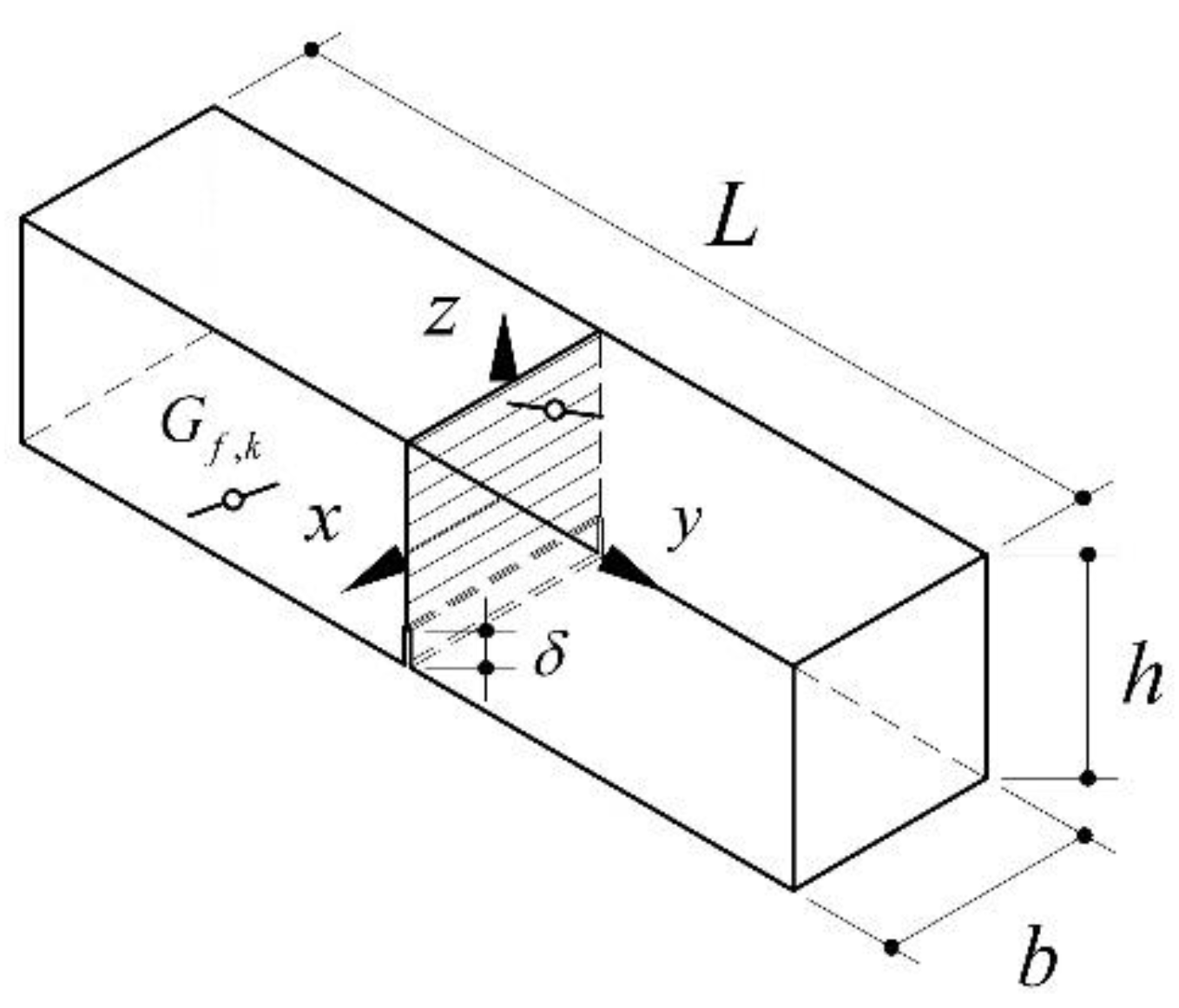
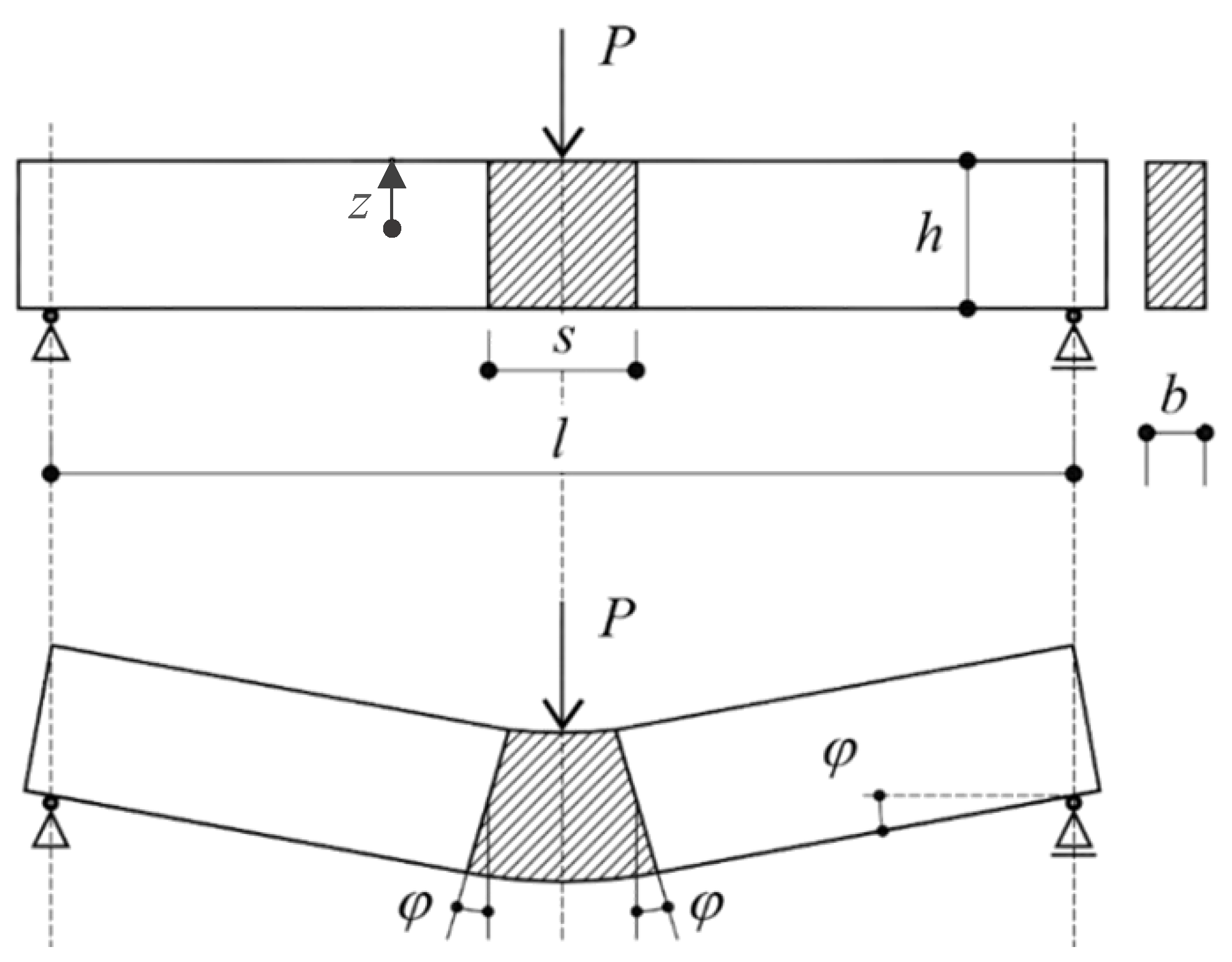
- The flexibility was distributed in the central part of the specimen for a length equal to “” while a rigid body behaviour was exhibited by the remaining end parts (Figure 2).
- (ii)
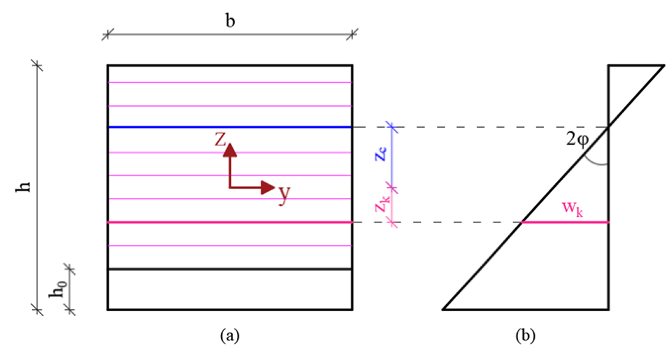
- The midspan cross-section was discretized in layers as shown in Figure 3. The average axial strain of the k-th layer, , before crack formation, and the crack-opening displacement, , after the crack formation, can be easily expressed for the k-th layer (k = 1, …, ) as in Equations (1) and (2).
- (iii)
- Consequently, the average value of the axial stress, , at k-th strip can be determined as a function of the axial deformation, , before cracking, or a function of the crack-opening displacements, , after cracking. The stress–strain and stress–displacement relationships assumed in this paper are reported in Section 3.2.2.
- (iv)
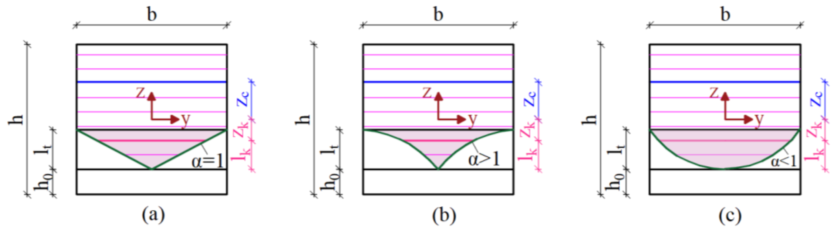
- A transition length, , was introduced in the notched cross-section (Figure 4), which starts from the top of the notch to the top of the integral part of the section, in order to consider the possible microdamage phenomena produced by the notching process. The mechanical meaning of this quantity is discussed in details in a previous paper [42] and omitted herein for the sake of brevity. Therefore, a reduced value of the width, , inside the transition zone was considered which can be evaluated with an exponential law as in Equation (3) where and are the distance of the k-th strip from the top of the notch and the coefficient of the exponential law, respectively:
- (v)
- The bridging effect offered by the fibres was taken in to account by introducing the action, , mobilised at the j-th step of the incremental analysis as in Equation (4):
3.2. Constitutive Laws Assumed in the Present Study
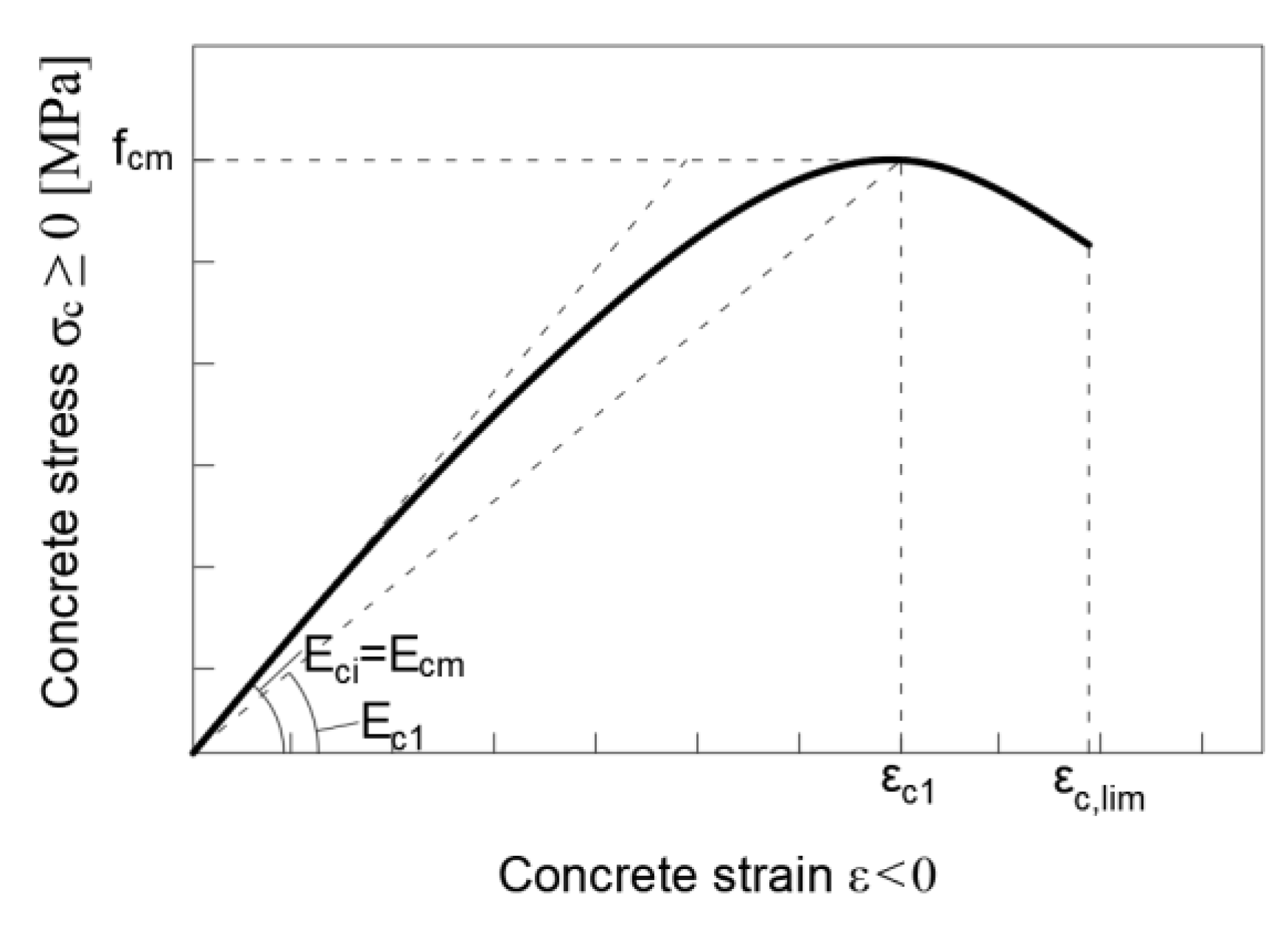
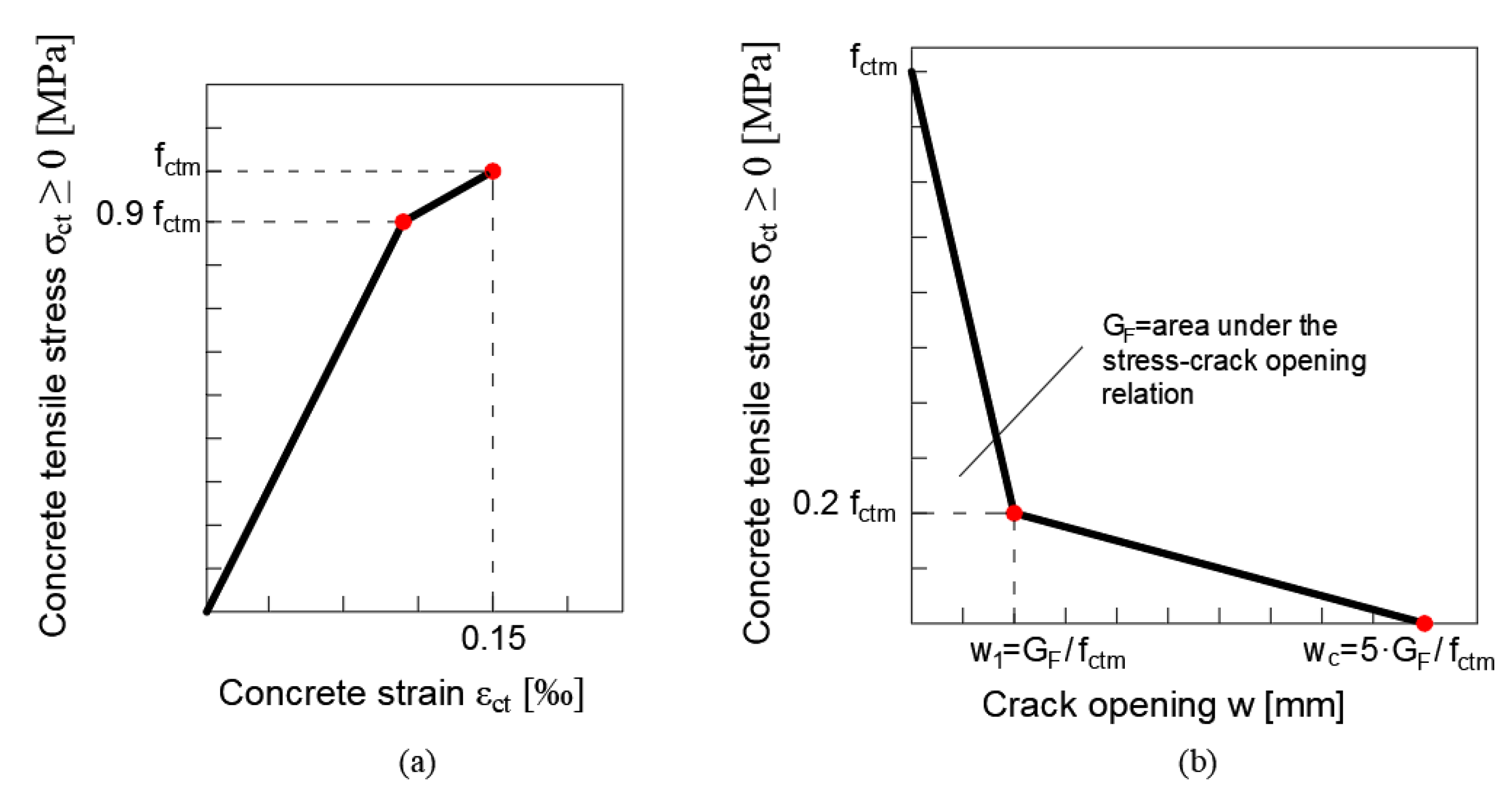
3.2.1. Stress–Strain Relationships for Concrete in Compression and in Tension
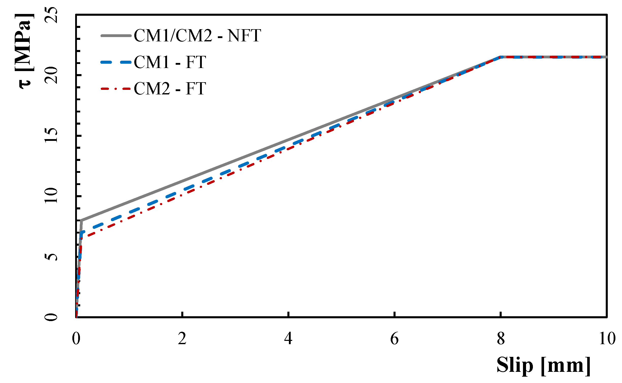
3.2.2. Modified Bond-Slip Model for Short Steel Fibres
- a linear-elastic behaviour up to the stress level corresponding to matrix tensile strength, identified by the two parameters , ;
- a hardening behaviour, characterized by the formation of many microcracks in the HPFRC mix, identified by the two parameters and ;
- a constant behaviour defined by the two parameters and .
4. Inverse Identification of the Relevant Material Laws
- In the first one, the cylindrical compression strength, , the transition length , and the exponential parameter, , were calibrated on the flexural response of the conditioned CM0 specimens (labelled CM0-FT). Experimentally, a 21% reduction in the cylindrical compression strength, , was observed on the conditioned specimens compared to not conditioned ones. This reduction was taken in account to calibrate the value of the transition length, , whose value, in the present model, was assumed equal to 85 mm (with an increase of 21% compared to that used in the previous model [42] in which the flexural behaviour of unconditioned CM0 specimens (labeled CM0-NFT) was predicted with a transition length, , equal to 70 mm). In both models, the coefficient of the exponential law, , was considered constant and equal to 0.40 (Table 3). Figure 7 shows both the average experimental curve (light-blue line) and the average numerical curve (pink line) obtained with the present model employed for the CM0-FT specimens.
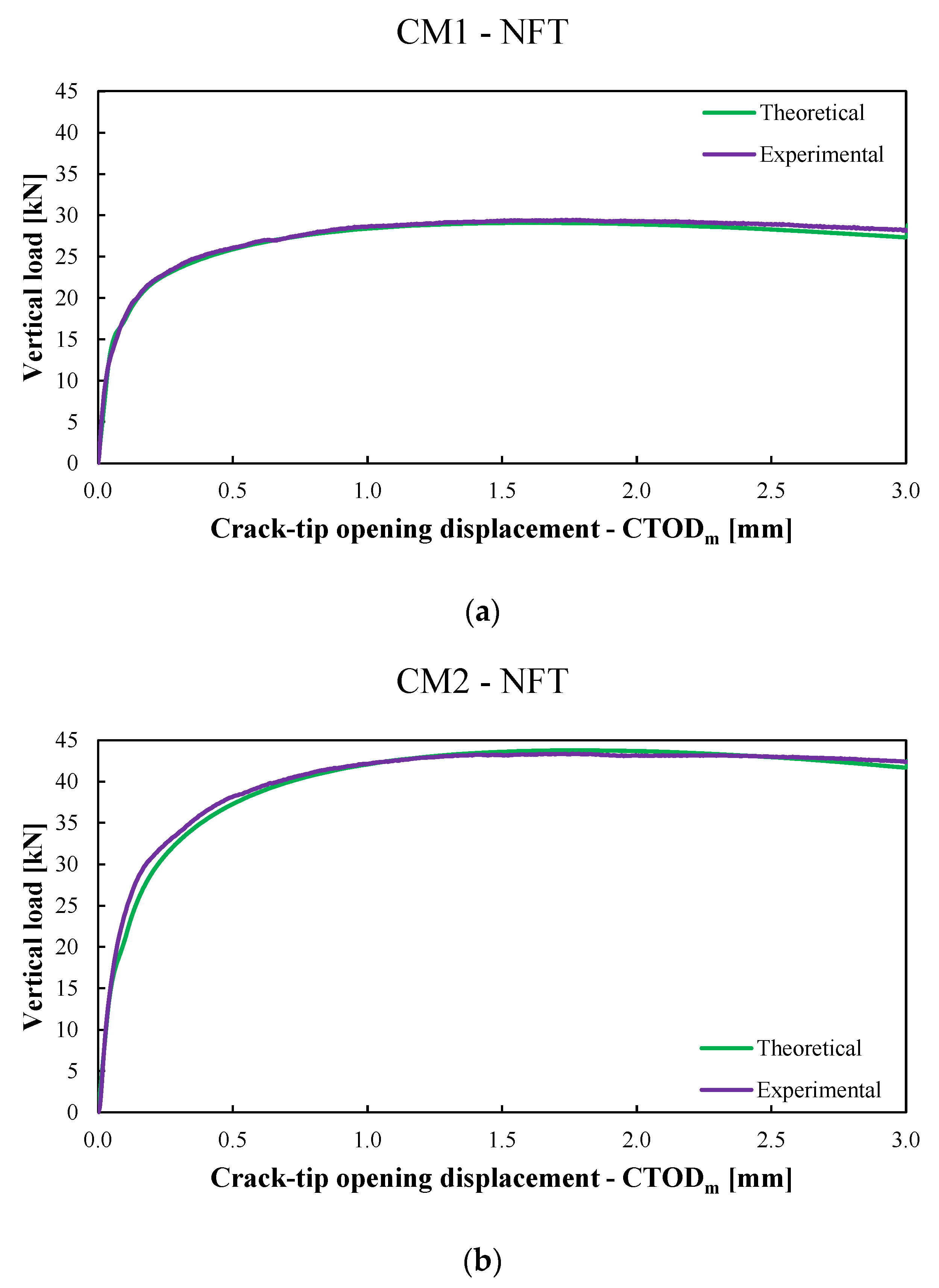
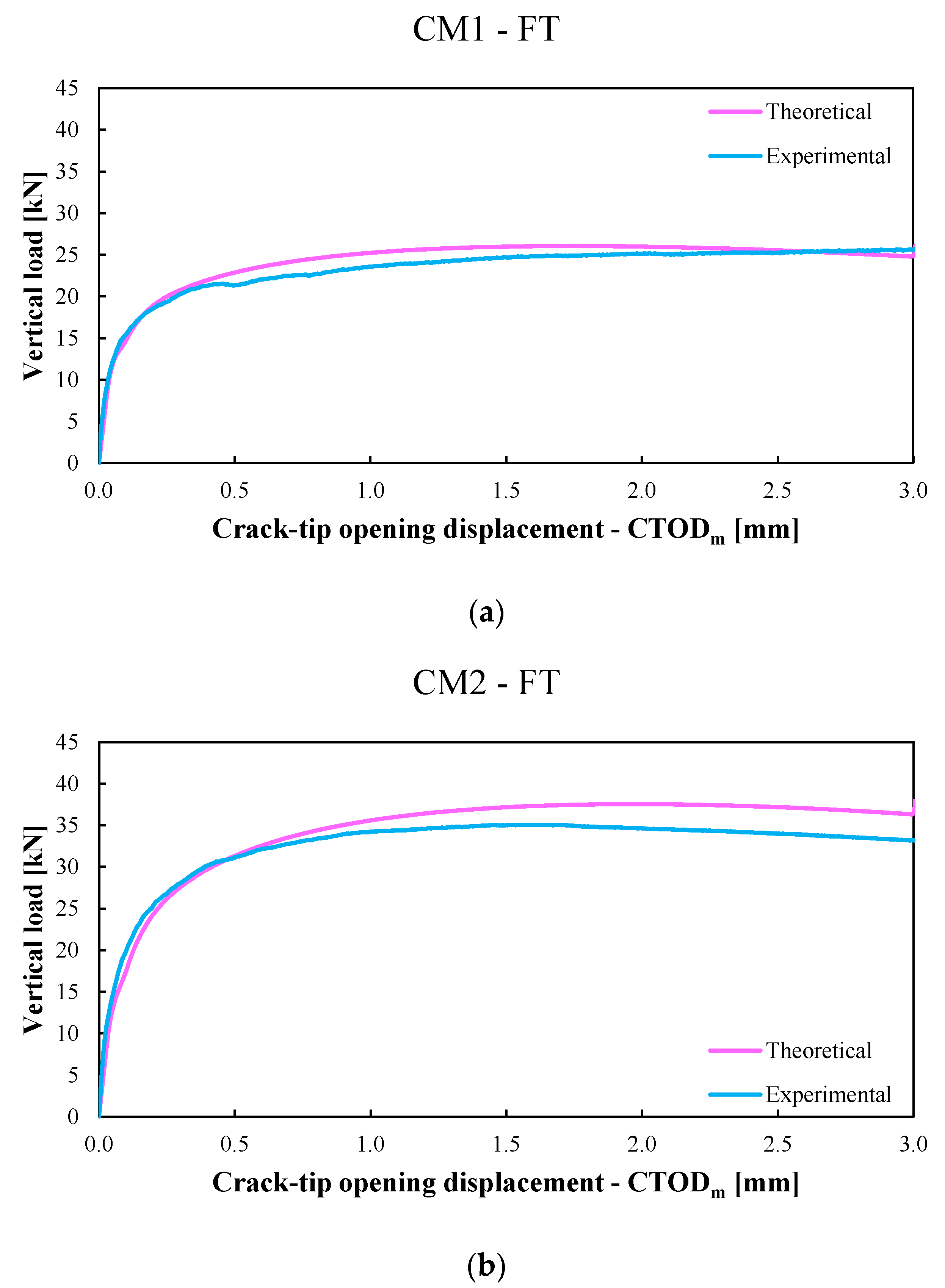
- In the second one, the six parameters of the bond-slip law (i.e., ) were calibrated on the flexural response of conditioned CM1 specimens (labelled CM1-FT). A 13% reduction in the parameter was adopted in the calibration of the conditioned specimens compared to the unconditioned ones.
- In the last one, only the parameter, , was calibrated again on the flexural response of conditioned CM2 specimens (labelled CM2-FT) while all the other parameters were considered constant. A 19% reduction in the parameter was adopted for the conditioned specimens compared to the unconditioned ones. Moreover, as in [42], a 20% reduction in the fibres’ volume fraction, , was considered in order to take into account the nonuniform fibre distribution.
5. Results
6. Conclusions
- The freeze–thaw cycles effect the cylindrical compression strength, , the transition length , and the bond-slip law of fibres, which confirms their significance as relevant parameters controlling the resulting response of HPFRC specimens;
- Table 3 shows that the compressive strength fcm undergoes a substantial reduction (in the order of 20%) as a result of the degradation processes induced by the FT cycles;
- as for the transition zone, which is a peculiar aspect of the considered model, a moderate increase in its the depth (from 70 mm to 85 mm) can be identified after the FT cycles, whereas its shape (controlled by the exponent α) does not change;
- Table 4 points out that the bond-slip law of fibres is also affected by the FT cycles, as, specifically, the elastic limit stress, τel, (and, consequently, the initial elastic stiffness of the same law) reduces by about 15%, with no changes in the other parameters;
- however, under the designers’ standpoint (and besides the specific values obtained in the present study), it should be noted that this change affects both serviceability and ultimate limit states in the structural response.
Author Contributions
Funding
Institutional Review Board Statement
Informed Consent Statement
Data Availability Statement
Conflicts of Interest
References
- Elsayed, M.; Tayeh, B.A.; Elmaaty, M.A.; Aldahsoory, Y.G. Behaviour of RC columns strengthened with Ultra-High Perfor-mance Fiber Reinforced concrete (UHPFRC) under eccentric loading. J. Build. Eng. 2022, 47, 103857. [Google Scholar] [CrossRef]
- Carlos Zanuy, C.; Irache, P.J.; García-Sainz, A. Composite Behavior of RC-HPFRC Tension Members under Service Loads. Materials 2021, 14, 47. [Google Scholar] [CrossRef] [PubMed]
- Cheng, J.; Luo, X.; Xiang, P. Experimental study on seismic behavior of RC beams with corroded stirrups at joints under cyclic loading. J. Build. Eng. 2020, 32, 101489. [Google Scholar] [CrossRef]
- Elmorsy, M.; Hassan, W.M. Seismic behavior of ultra-high performance concrete elements: State-of-the-art review and test database and trends. J. Build. Eng. 2021, 40, 102572. [Google Scholar] [CrossRef]
- Sharma, R.; Pal Bansal, P. Experimental investigation of initially damaged beam column joint retrofitted with reinforced UHP-HFRC overlay. J. Build. Eng. 2022, 49, 103973. [Google Scholar] [CrossRef]
- Pereiro-Barceló, J.; Bonet, J.L.; Cabañero-Escudero, B.; Martínez-Jaén, B.B. Cyclic behavior of hybrid RC columns using High-Performance Fiber-Reinforced Concrete and Ni-Ti SMA bars in critical regions. Compos. Struct. 2019, 212, 207–219. [Google Scholar] [CrossRef]
- O’Hegarty, R.; Kinnane, O.; Newell, J.; West, R. High performance, low carbon concrete for building cladding applications. J. Build. Eng. 2021, 43, 102566. [Google Scholar] [CrossRef]
- Juhasz, P.K.; Schaul, P. Design of Industrial Floors—TR34 and Finite Element Analysis (Part 2). J. Civ. Eng. Archit. 2019, 13, 512–522. [Google Scholar] [CrossRef]
- Foglar, M.; Hajek, R.; Fladr, J.; Pachman, J.; Stoller, J. Full-scale experimental testing of the blast resistance of HPFRC and UHPFRC bridge decks. Constr. Build. Mater. 2017, 145, 588–601. [Google Scholar] [CrossRef]
- Tufekci, M.M.; Gokce, A. Development of heavyweight high performance fiber reinforced cementitious composites (HPFRCC)-Part II: X-ray and gamma radiation shielding properties. Constr. Build Mater. 2018, 163, 326–336. [Google Scholar] [CrossRef]
- Liao, Q.; Yu, J.; Xie, X.; Ye, J.; Jiang, F. Experimental study of reinforced UHDC-UHPC panels under close-in blast loading. J. Build. Eng. 2022, 46, 103498. [Google Scholar] [CrossRef]
- Chu, S.H. Development of Infilled Cementitious Composites (ICC). Compos. Struct. 2021, 267, 113885. [Google Scholar] [CrossRef]
- Savino, V.; Lanzoni, L.; Tarantino, A.M.; Viviani, M. An extended model to predict the compressive, tensile and flexural strengths of HPFRCs and UHPFRCs: Definition and experimental validation. Compos. Part B Eng. 2019, 163, 681–689. [Google Scholar] [CrossRef]
- Savino, V.; Lanzoni, L.; Tarantino, A.M.; Viviani, M. Simple and effective models to predict the compressive and tensile strength of HPFRC as the steel fiber content and type changes. Compos. Part B Eng. 2018, 137, 153–162. [Google Scholar] [CrossRef]
- Ashkezari, G.D.; Fotouhi, F.; Razmara, M. Experimental relationships between steel fiber volume fraction and mechanical properties of ultra-high performance fiber-reinforced concrete, J. Build. Eng. 2020, 32, 101613. [Google Scholar] [CrossRef]
- Caggiano, A.; Folino, P.; Lima, C.; Martinelli, E.; Pepe, M. On the mechanical response of Hybrid Fiber Reinforced Concrete with Recycled and Industrial Steel Fibers. Constr. Build. Mater. 2017, 147, 286–295. [Google Scholar] [CrossRef]
- Caggiano, A.; Gambarelli, S.; Martinelli, E.; Nisticò, N.; Pepe, M. Experimental characterization of the post-cracking response in Hybrid Steel/Polypropylene Fiber-Reinforced Concrete. Constr. Build. Mater. 2016, 125, 1035–1043. [Google Scholar] [CrossRef]
- Kim, D.J.; Naaman, A.E.; El-Tawil, S. Comparative flexural behavior of four fiber reinforced cementitious composites. Cem. Concr. Compos. 2008, 30, 917–928. [Google Scholar] [CrossRef]
- Uchida, Y.; Takeyama, T.; Dei, T. Ultra High Strength Fiber Reinforced Concrete Using Aramid Fiber. In Fracture Mechanics of Concrete and Concrete Structures—High Performance, Fiber Reinforced Concrete, Special Loadings and Structural Applications; Korea Concrete Institute: Seoul, Korea, 2010; pp. 1492–1497. [Google Scholar]
- Foti, D. Use of recycled waste pet bottles fibers for the reinforcement of concrete. Compos. Struct. 2013, 96, 396–404. [Google Scholar] [CrossRef]
- Choi, J.-I.; Song, K.-I.; Song, J.-K.; Lee, B.Y. Composite properties of high-strength polyethylene fiber-reinforced cement and cementless composites. Compos. Struct. 2016, 138, 116–121. [Google Scholar] [CrossRef]
- Savastano, H.; Warden, P.G.; Coutts, R.S.P. Mechanically pulped sisal as reinforcement in cementitious matrices. Cem. Concr. Compos. 2003, 25, 311–319. [Google Scholar] [CrossRef]
- Li, Z.; Wang, X.; Wang, L. Properties of hemp fibre reinforced concrete composites. Compos. Part A Appl. Sci. Manuf. 2006, 37, 497–505. [Google Scholar] [CrossRef]
- Wang, W.; Chouw, N. The behaviour of coconut fibre reinforced concrete (CFRC) under impact loading. Constr Build Mater 2017, 134, 452–461. [Google Scholar] [CrossRef]
- Smarzewski, P. Flexural Toughness of High-Performance Concrete with Basalt and Polypropylene Short Fibers. Adv Civ Eng. 2018, 5024353. [Google Scholar]
- Smarzewski, P. Influence of basalt-polypropylene fibres on fracture properties of high performance concrete. Compos. Struct. 2019, 209, 23–33. [Google Scholar] [CrossRef]
- Reis, J.; Ferreira, A. Assessment of fracture properties of epoxy polymer concrete reinforced with short carbon and glass fibers. Constr. Build. Mater. 2004, 18, 523–528. [Google Scholar] [CrossRef]
- Brandt, A.M. Fibre reinforced cement-based (FRC) composites after over 40 years of development in building and civil engi-neering. Compos. Struct. 2008, 86, 3–9. [Google Scholar]
- Zollo, R.F. Fiber-reinforced concrete: An overview after 30 years of development. Cem. Concr. Compos. 1997, 19, 107–122. [Google Scholar] [CrossRef]
- Kim, J.; Kim, D.J.; Park, S.H.; Zi, G. Investigating the flexural resistance of fiber reinforced cementitious composites under biaxial condition. Compos. Struct. 2015, 122, 198–208. [Google Scholar] [CrossRef]
- Cho, T. Prediction of cyclic freeze–thaw damage in concrete structures based on response surface method. Constr. Build. Mater. 2007, 21, 2031–2040. [Google Scholar] [CrossRef]
- Shang, H.S.; Song, Y.P. Experimental study of strength and deformation of plain concrete under biaxial compression after freezing and thawing cycles. Cem. Concr. Res. 2006, 36, 1857–1864. [Google Scholar] [CrossRef]
- Jang, J.G.; Kim, H.K.; Kim, T.S.; Min, B.J.; Lee, H.K. Improved flexural fatigue resistance of PVA fiber-reinforced concrete subjected to freezing and thawing cycles. Constr. Build. Mater. 2014, 59, 129–135. [Google Scholar] [CrossRef]
- Zhang, W.M.; Zhang, N.; Zhou, Y. Effect of flexural impact on freeze–thaw and deicing salt resistance of steel fiber reinforced concrete. Mater. Struct. 2016, 49, 5161–5168. [Google Scholar] [CrossRef]
- Song, H.-W.; Kwon, S.-J. Evaluation of chloride penetration in high performance concrete using neural network algorithm and micro pore structure. Cem. Concr. Res. 2009, 39, 814–824. [Google Scholar] [CrossRef]
- Ismail, M.; Ohtsu, M. Corrosion rate of ordinary and high-performance concrete subjected to chloride attack by AC impedance spectroscopy. Constr. Build. Mater. 2006, 20, 458–469. [Google Scholar] [CrossRef]
- Feo, L.; Ascione, F.; Penna, R.; Lau, D.; Lamberti, M. An experimental investigation on freezing and thawing durability of high performance fiber reinforced concrete (HPFRC). Compos. Struct. 2020, 234, 111673. [Google Scholar] [CrossRef]
- Zhao, Y.-R.; Wang, L.; Lei, Z.-K.; Han, X.-F.; Shi, J.-N. Study on bending damage and failure of basalt fiber reinforced concrete under freeze-thaw cycles. Constr. Build. Mater. 2018, 163, 460–470. [Google Scholar] [CrossRef]
- Ameri, F.; de Brito, J.; Madhkhan, M.; Ali Taheri, R. Steel fibre-reinforced high-strength concrete incorporating copper slag: Mechanical, gamma-ray shielding, impact resistance, and microstructural characteristics. J. Build. Eng. 2020, 29, 101118. [Google Scholar] [CrossRef]
- Lee, S.-T.; Park, S.-H.; Kim, D.-G.; Kang, J.-M. Effect of Freeze–Thaw Cycles on the Performance of Concrete Containing Water-Cooled and Air-Cooled Slag. Appl. Sci. 2021, 11, 7291. [Google Scholar] [CrossRef]
- Vivek, D.; Elango, K.S.; Gokul Prasath, K.; Ashik Saran, V.; Ajeeth Divine Chakaravarthy, V.B.; Abimanyu, S. Mechanical and durability studies of high performance concrete (HPC) with nano-silica. Mater. Today Proc. 2021, 52, 388–390. [Google Scholar] [CrossRef]
- Martinelli, E.; Pepe, M.; Penna, R.; Feo, L. A Cracked-Hinge approach to modelling High Performance Fiber-Reinforced Concrete. Compos. Struct. 2021, 273, 114277. [Google Scholar] [CrossRef]
- Martinelli, E.; Pepe, M.; Fraternali, F. Meso-Scale Formulation of a Cracked-Hinge Model for Hybrid Fiber-Reinforced Cement Composites. Fibers 2020, 8, 56. [Google Scholar] [CrossRef]
- Hillerborg, A. Application of the fictitious crack model to different types of materials. Int. J. Fract. 1991, 51, 95–102. [Google Scholar] [CrossRef]
- Kytinou, V.K.; Chalioris, C.E.; Karayannis, C.G. Analysis of Residual Flexural Stiffness of Steel Fiber-Reinforced Concrete Beams with Steel Reinforcement. Materials 2020, 13, 2698. [Google Scholar] [CrossRef]
- Hillerborg, A.; Modéer, M.; Petersson, P.-E. Analysis of crack formation and crack growth in concrete by means of fracture mechanics and finite elements. Cem. Concr. Res. 1976, 6, 773–781. [Google Scholar] [CrossRef]
- Olesen, J.F. Fictitious Crack Propagation in Fiber-Reinforced Concrete Beams. J. Eng. Mech. 2001, 127, 272–280. [Google Scholar] [CrossRef]
- Armelin, H.S.; Banthia, N. Predicting the flexural postcracking performance of steel fiber reinforced concrete from the pullout of single fibers. Mater. J. 1997, 94, 18–31. [Google Scholar]
- Bekaert S.p.A. Available online: www.bekaert.com (accessed on 1 July 2022).
- Kerakoll S.p.A. Available online: www.kerakoll.com (accessed on 1 July 2022).
- UNI 7087-2017; Concrete-Determination of the Resistance to the Degrade Due to Freeze-Thaw Cycles. UNI: Milan, Italy, 2017.
- UNI 11039-2; Steel, Fibre Reinforced Concrete-Test Method for Determination of First Crack Strength and Ductility Indexes. UNI: Milan, Italy, 2003.
- UNI EN 12390-4; Testing Hardened Concrete. Part 4: Compressive Strength-Specification for Testing Machines. iTeh Standards: Etobicoke, ON, Canada, 2000.
- fib Bulletin No. 42. Constitutive Modelling of High Strength/High Performance Concrete; State-of-Art Report; International Federation for Structural Concrete: Lausanne, Switzerland, 2008; 130p, ISBN 978-2-88394-082-6.
- Tai, Y.-S.; El-Tawil, S. High loading-rate pullout behavior of inclined deformed steel fibers embedded in ultra-high performance concrete. Constr. Build. Mater. 2017, 148, 204–218. [Google Scholar] [CrossRef]


| Mix. | ||||||||
|---|---|---|---|---|---|---|---|---|
| [kN] | [kN] | [MPa] | [MPa] | [MPa] | [MPa] | [MPa] | [MPa] | |
| CM0 | 11.213 | 9.105 | 3.05 | 2.477 | - | - | - | - |
| CM1 | 14.489 | 12.538 | 4.013 | 3.475 | 6.617 | 5.435 | 7.99 | 6.845 |
| CM2 | 18.595 | 16.175 | 5.06 | 4.327 | 9.15 | 7.537 | 11.473 | 9.255 |
| Mix. | ||||||||
|---|---|---|---|---|---|---|---|---|
| [kNmm] | [kNmm] | [kNmm] | [kNmm] | [-] | [-] | [-] | [-] | |
| CM1 | 14,283.43 | 11,742.40 | 69,226.73 | 59,175.15 | 1.647 | 1.565 | 1.265 | 1.265 |
| CM2 | 20,508.47 | 16,895.83 | 102,877.93 | 82,992.00 | 1.837 | 1.747 | 1.257 | 1.250 |
| Specimen Designation | Model | |||
|---|---|---|---|---|
| [MPa] | [mm] | [-] | ||
| CM0-NFT | 53.0 | 70.0 | 0.4 | Ref. [42] |
| CM0-FT | 42.0 | 85.0 | 0.4 | Present paper |
| Series | Model | ||||||
|---|---|---|---|---|---|---|---|
| [mm] | [mm] | [mm] | [MPa] | [MPa] | [MPa] | ||
| CM1-NFT | 0.10 | 8.00 | 10.00 | 8.00 | 21.50 | 21.50 | Ref. [42] |
| CM1-FT | 0.10 | 8.00 | 10.00 | 7.00 | 21.50 | 21.50 | Present paper |
| CM2-NFT | 0.10 | 8.00 | 10.00 | 8.00 | 21.50 | 21.50 | Ref. [42] |
| CM2-FT | 0.10 | 8.00 | 10.00 | 6.50 | 21.50 | 21.50 | Present paper |
| Results | CM1 | CM2 | ||||||
|---|---|---|---|---|---|---|---|---|
| [MPa] | [MPa] | [MPa] | [MPa] | [MPa] | [MPa] | [MPa] | [MPa] | |
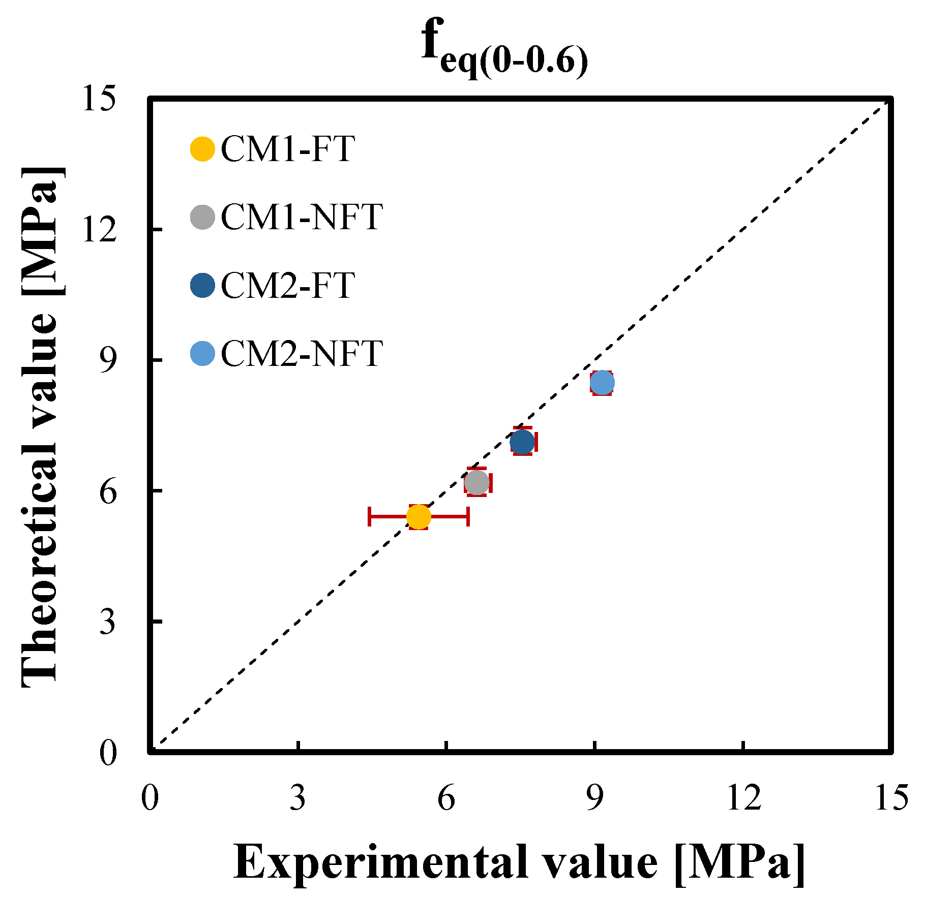
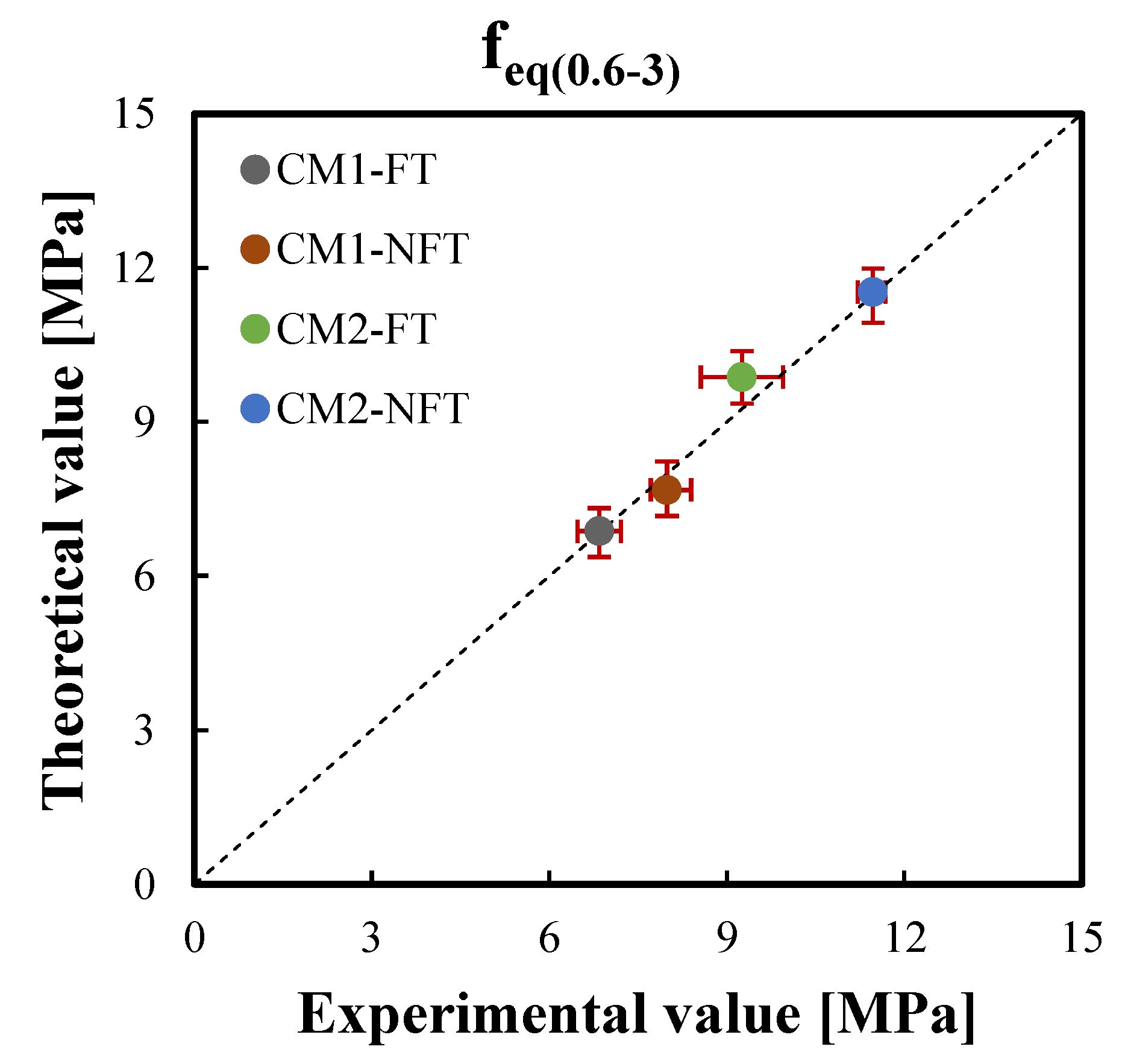
| Experimental | 6.617 | 5.435 | 7.990 | 6.845 | 9.150 | 7.537 | 11.473 | 9.255 |
| Theoretical | 6.179 | 5.411 | 7.672 | 6.871 | 8.486 | 7.125 | 11.532 | 9.871 |
| Percentage difference (%) | 6.61 | 0.45 | 3.98 | 0.39 | 7.26 | 5.47 | 0.51 | 6.66 |
| Results | CM1 | CM2 | ||||||
|---|---|---|---|---|---|---|---|---|
| [kNmm] | [kNmm] | [kNmm] | [kNmm] | [kNmm] | [kNmm] | [kNmm] | [kNmm] | |
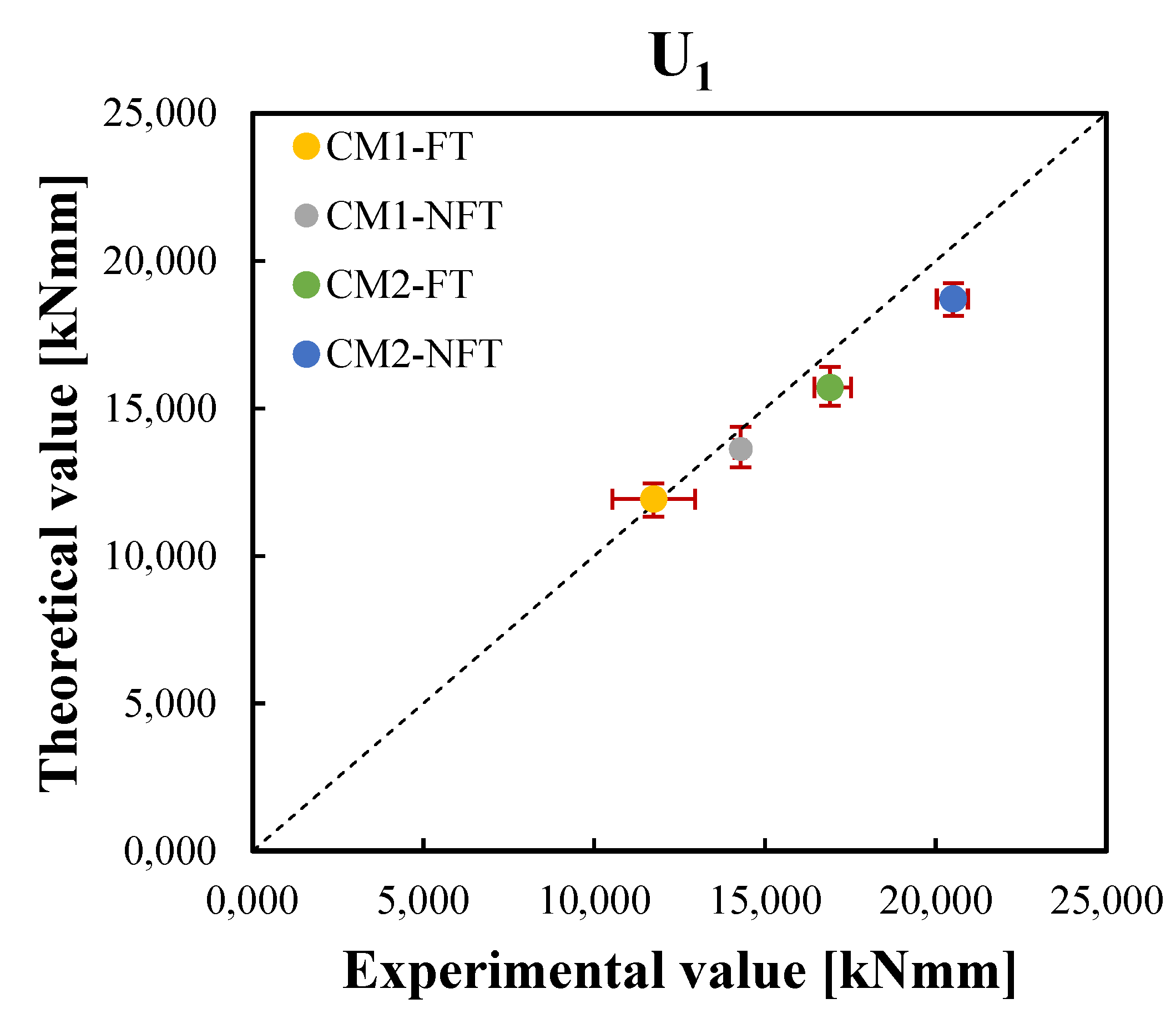
| Experimental | 14,283.43 | 11,742.40 | 69,226.73 | 59,175.15 | 20,508.47 | 16,895.83 | 102,877.93 | 82,992.00 |
| Theoretical | 13,625.51 | 11,930.62 | 67,667.93 | 60,606.61 | 18,711.24 | 15,709.63 | 101,710.39 | 87,061.56 |
| Percentage difference (%) | 4.61 | 1.60 | 2.25 | 2.42 | 8.76 | 7.02 | 1.13 | 4.90 |
Publisher’s Note: MDPI stays neutral with regard to jurisdictional claims in published maps and institutional affiliations. |
© 2022 by the authors. Licensee MDPI, Basel, Switzerland. This article is an open access article distributed under the terms and conditions of the Creative Commons Attribution (CC BY) license (https://creativecommons.org/licenses/by/4.0/).
Share and Cite
Penna, R.; Feo, L.; Martinelli, E.; Pepe, M. Theoretical Modelling of the Degradation Processes Induced by Freeze–Thaw Cycles on Bond-Slip Laws of Fibres in High-Performance Fibre-Reinforced Concrete. Materials 2022, 15, 6122. https://doi.org/10.3390/ma15176122
Penna R, Feo L, Martinelli E, Pepe M. Theoretical Modelling of the Degradation Processes Induced by Freeze–Thaw Cycles on Bond-Slip Laws of Fibres in High-Performance Fibre-Reinforced Concrete. Materials. 2022; 15(17):6122. https://doi.org/10.3390/ma15176122
Chicago/Turabian StylePenna, Rosa, Luciano Feo, Enzo Martinelli, and Marco Pepe. 2022. "Theoretical Modelling of the Degradation Processes Induced by Freeze–Thaw Cycles on Bond-Slip Laws of Fibres in High-Performance Fibre-Reinforced Concrete" Materials 15, no. 17: 6122. https://doi.org/10.3390/ma15176122
APA StylePenna, R., Feo, L., Martinelli, E., & Pepe, M. (2022). Theoretical Modelling of the Degradation Processes Induced by Freeze–Thaw Cycles on Bond-Slip Laws of Fibres in High-Performance Fibre-Reinforced Concrete. Materials, 15(17), 6122. https://doi.org/10.3390/ma15176122