
Evaluation of Corrosion Residual Life Prediction Methods for Metal Pipelines

Abstract
:1. Introduction
 , the pipeline corrosion rate is regarded as an uncertain and random value, and the residual life of the corroded pipeline has been predicted by studying the distribution model of the maximum corrosion depth data, which mainly includes GEV distribution, Gumbel distribution, Frechet distribution, and Weibull distribution. Zhang X S et al. [1] established a residual life prediction model of corroded oil and gas pipelines based on improved GEV distribution. Firstly, the Markov Chain Monte Carlo (MCMC) method was used to estimate the parameters of the GEV distribution function and determine the type of extreme value distribution. When the graphic test was found to be reasonable, then the distribution could be used to predict the maximum corrosion depth. Secondly, a corrosion allowance prediction model was established based on the reliability and safety of the pipeline. Finally, according to the data of the maximum corrosion depth, corrosion allowance and annual service life of the pipeline, the relationship index model of the three was established to predict the residual life of the pipeline. Based on Gumbel distribution, Zhang X S et al. [2] processed the maximum corrosion depth data randomly selected from the inspection data of an oil and gas pipeline, established the prediction model of the maximum corrosion depth of the pipeline, and then estimated the value of the parameters of the prediction model with the Markov Chain Monte Carlo (MCMC) method and predicted the possible maximum corrosion depth through the model. Hence, based on the obtained corrosion depth, critical corrosion depth and pipeline service life and other data, the relationship index model between the three was established to predict the residual life of oil and gas pipelines. Wang R et al. [3,4] realized the scientific evaluation and prediction of the corrosion status and operation of offshore oil and gas pipelines by utilizing Frechet extreme value distribution to establish the prediction model of the maximum corrosion depth of offshore oil and gas pipelines, combined it with the Monte Carlo (MC) method to estimate the parameter value of the prediction model and predict the possible maximum corrosion depth, and analyzed and predicted the maximum probability of pipe wall corrosion through the Markov Chain model. Similarly, F. Caleyo et al. [5] used the Monte Carlo simulations to study the probability distributions of external corrosion pit depth and pit growth rate in underground pipelines and combined a predictive pit growth model with the observed distributions of the model variables in a range of soils. Depending on the pipeline age, any of the three maximal extreme value distributions, i.e., Weibull, Fréchet or Gumbel, can arise as the best fit to the pitting depth and rate data.
 is based on the reliability theory, using the ultimate limit state function to establish the mathematical probability model of pipeline failure, and predict the residual life of the pipeline and the cumulative failure probability at a given time. Shuai J [6] regarded various factors affecting the residual life of pipelines as random variables with different distributions, and established a mathematical probability model to predict pipeline failure. Using this model, the effects of corrosion rate, defect depth, pipe wall thickness, and working pressure on the reliability of the pipeline were studied. The corrosion rate obtained from the analysis can reasonably predict the safety status of the whole pipeline. Yu S R et al. [7] established a probability model for predicting the residual life of pipeline corrosion based on the shell-92 deterministic model. The Monte Carlo method was used to calculate the residual life of the pipeline and its cumulative distribution function, and the parameter sensitivity analysis was carried out. The main parameters affecting the corrosion residual life of the buried pipeline and their variation with the service time were discussed. Alma Valor et al. [8] derived different corrosion rate distributions from various corrosion growth models and used these to perform reliability analyses of underground pipelines. Hu Q F et al. [9] proposed a nonlinear prediction model for the maximum corrosion depth of gas pipelines under different sample independence by using the Bayesian estimation method based on the probability distribution of model parameters, and solved the model by using the MCMC method. Luo J H et al. [10] used the size data of nearly 1000 corrosion overhaul defects of a pipeline over the years to calculate the corrosion rate distribution of the pipeline and establish a probability distribution model of corrosion rate. Based on the reliability theory, the corrosion residual life of the pipeline was predicted by using the limit defect size data determined by the corrosion residual strength evaluation. Additionally, three deterministic and probabilistic models were introduced by Markus R. Dann et al. [11] to account for the sizing bias present in in-line inspection data for corrosion growth analysis.
  is based on historical statistical data such as corrosion rate and remaining thickness, using different modeling theories and methods to explore the change rules in the historical data, and extrapolating the data in the timeline to predict the residual life of the pipeline. The Modeling methods and theories used in this kind of research mainly include the BP neural network modeling method, gray theory modeling method, exponential smoothing method and time series prediction method. Using the grey theory, Yu X C et al. [12] proposed effectively predicting the corrosion rate via the complex mapping relationship between the corrosion rate and the corrosion influencing factors in the water injection pipeline. At the same time, to improve the prediction accuracy, the standard GM (1,1) model was reasonably improved, in order to predict the change trend of the corrosion rate with time. Wang H T et al. [13] used the cubic exponential smoothing method to establish the prediction model of the pipeline corrosion rate, fitted and predicted the corrosion rate data, and obtained the most reasonable weight coefficient in the prediction model α. Then, through the comparative analysis with the primary exponential smoothing method and the quadratic exponential smoothing method, it was concluded that the cubic exponential smoothing method has higher prediction accuracy and that the predicted value is consistent with the actual value. Kevin S et al. [14] utilized historical excavation and recoat information to identify static defects and quantify systemic bias between inspections. To reduce differences in reporting and the analyst interpretation of the recorded magnetic signals, novel analysis techniques were employed to normalize the data sets against each other. The resulting uncertainty of the corrosion growth rates was then further reduced by deriving and applying a regression model to reduce the effect of the different sizing models and the identified systemic bias. Liu X N [15] established the quantitative relationship between corrosion residual life and corrosion rate, coefficient of variation, corrosion allowance and reliability, and obtained the calculation formula to determine the corrosion residual life. Zhang X S et al. [16] analyzed the feasibility of building a grey theory model, established a GM (1,1) model with optimized parameters, changed the initial conditions of the model, and predicted the corrosion depth of submarine pipelines. According to the predicted corrosion depth, the Markov model was used to quantitatively analyze the future corrosion state of the submarine pipeline and predict its residual life. Xiao W et al. [17] determined the corrosion risk prediction method suitable for the Tahe Oilfield by comparing the application scope, reliability and economy of five common pipeline corrosion risk prediction methods. The classical BP neural network algorithm was optimized with the help of a genetic algorithm, which effectively improves the accuracy and reliability of the BP neural network. Yao Q [18] used the historical data collected on site, combined with the characteristics of the corrosion problem, and adopted the time series model to predict the corrosion rate. On this basis, he used the Monte Carlo method to evaluate the residual life of the equipment, and judged the residual service life of the equipment through the statistics of the corrosion failure probability of the equipment, so as to obtain the residual life of the equipment., category can reflect the relationship of corrosion degree with time more directly. Meanwhile, compared with category , category can directly provide the residual life of the pipeline under the current corrosion condition, but not the reliability or failure probability of the residual life. At present, most of the researches who prefer category of methods focus on the selection of modeling methods and theories. However, the lack of comparative studies using the same basic statistical data and different modeling methods and theories makes it challenging to objectively and quantitatively assess the benefits and drawbacks of the prediction accuracy of each method. Based on the same basic statistical data, this study uses a variety of modeling methods and theories to establish residual life prediction models. By comparing the accuracy of the predictions, it then discusses the applicability and reliability of each modeling method and theory.
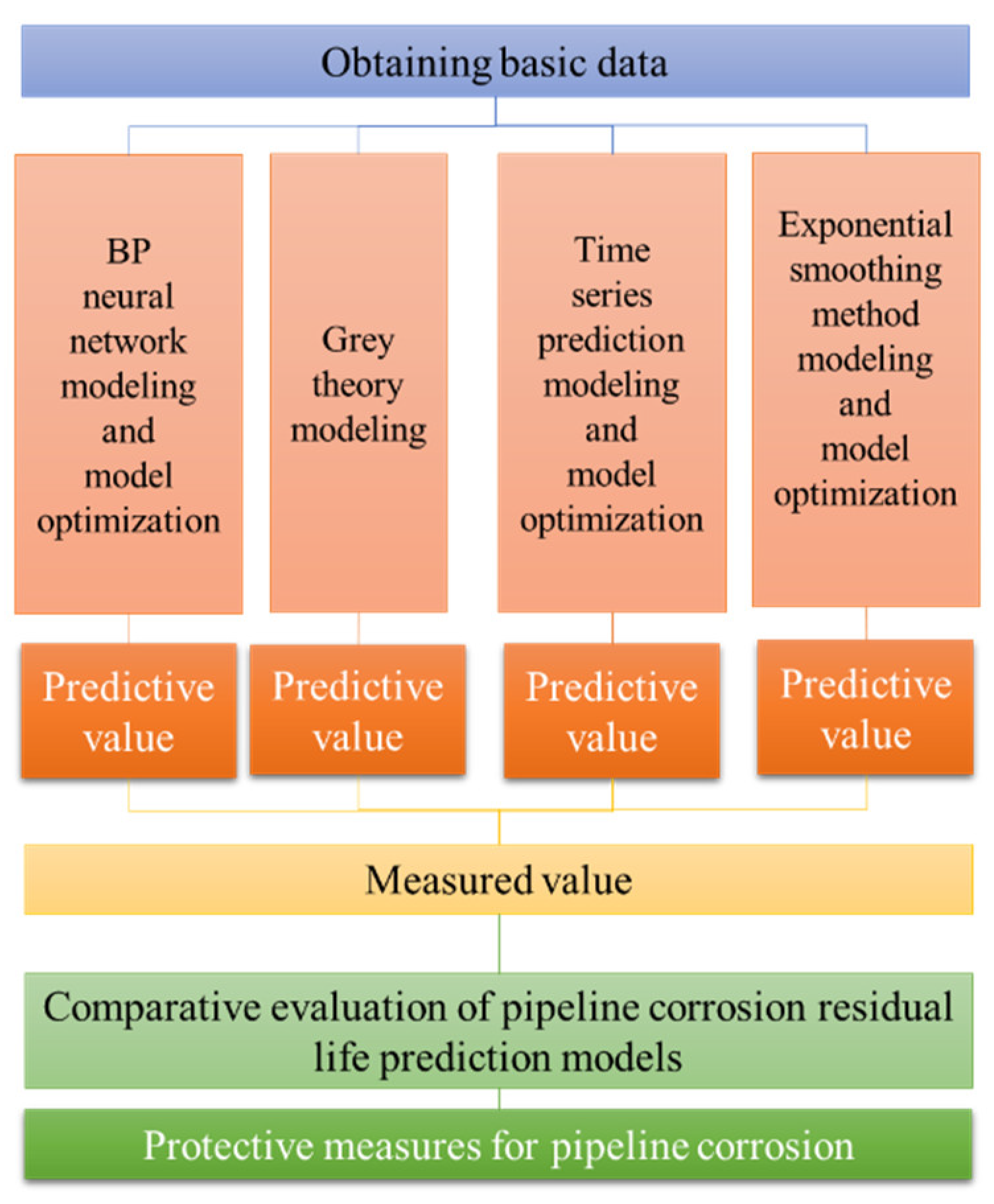
2. Prediction Method of Residual Life of Metal Pipe
3. Modeling Methods and Theories
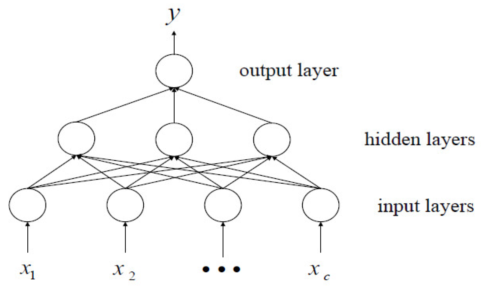
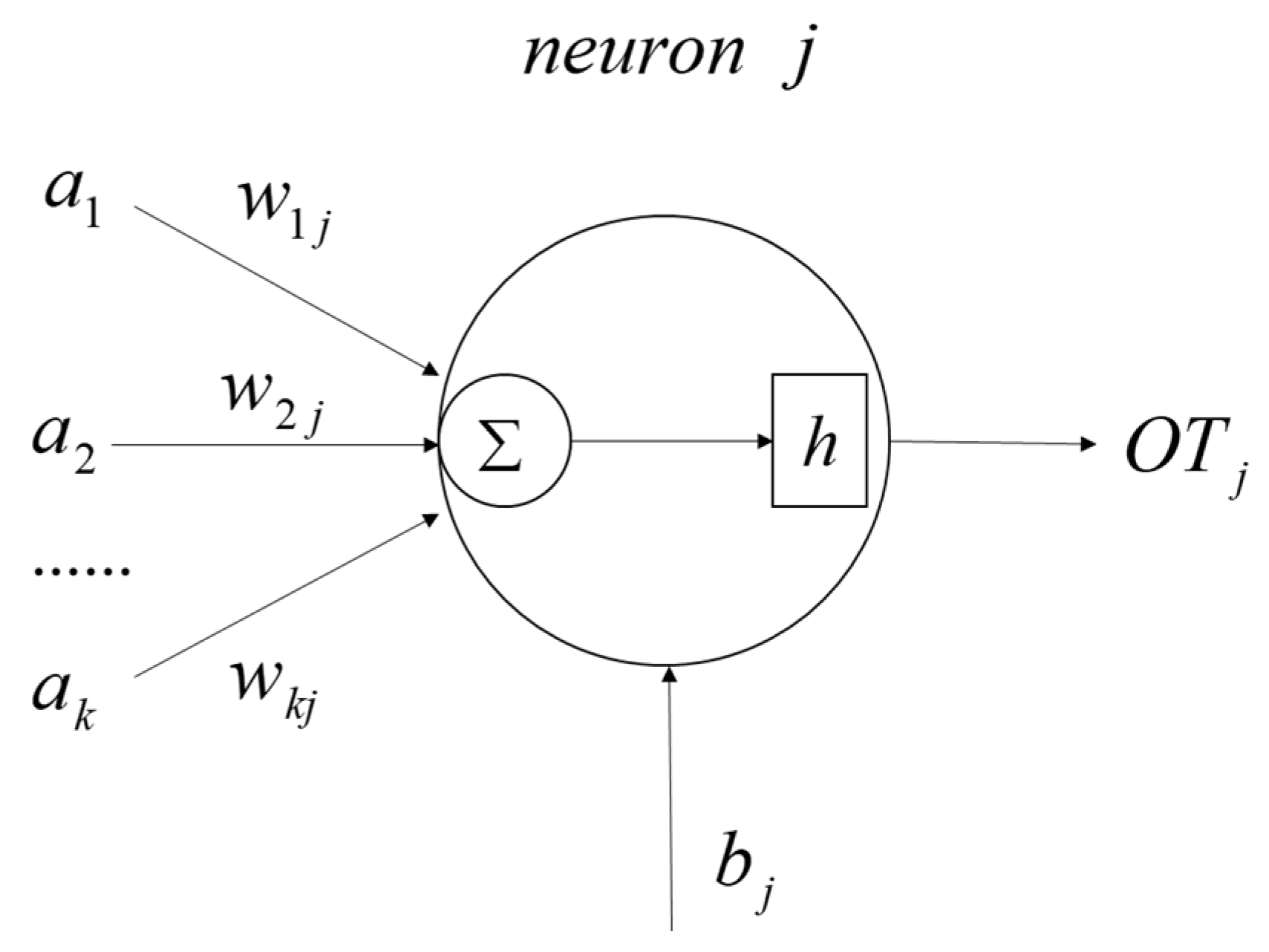
3.1. The BP Neural Network Modeling
3.2. The Grey Theory Modeling
3.3. The Time Series Prediction Modeling
3.4. The Exponential Smoothing Method Modeling
4. Case Analysis
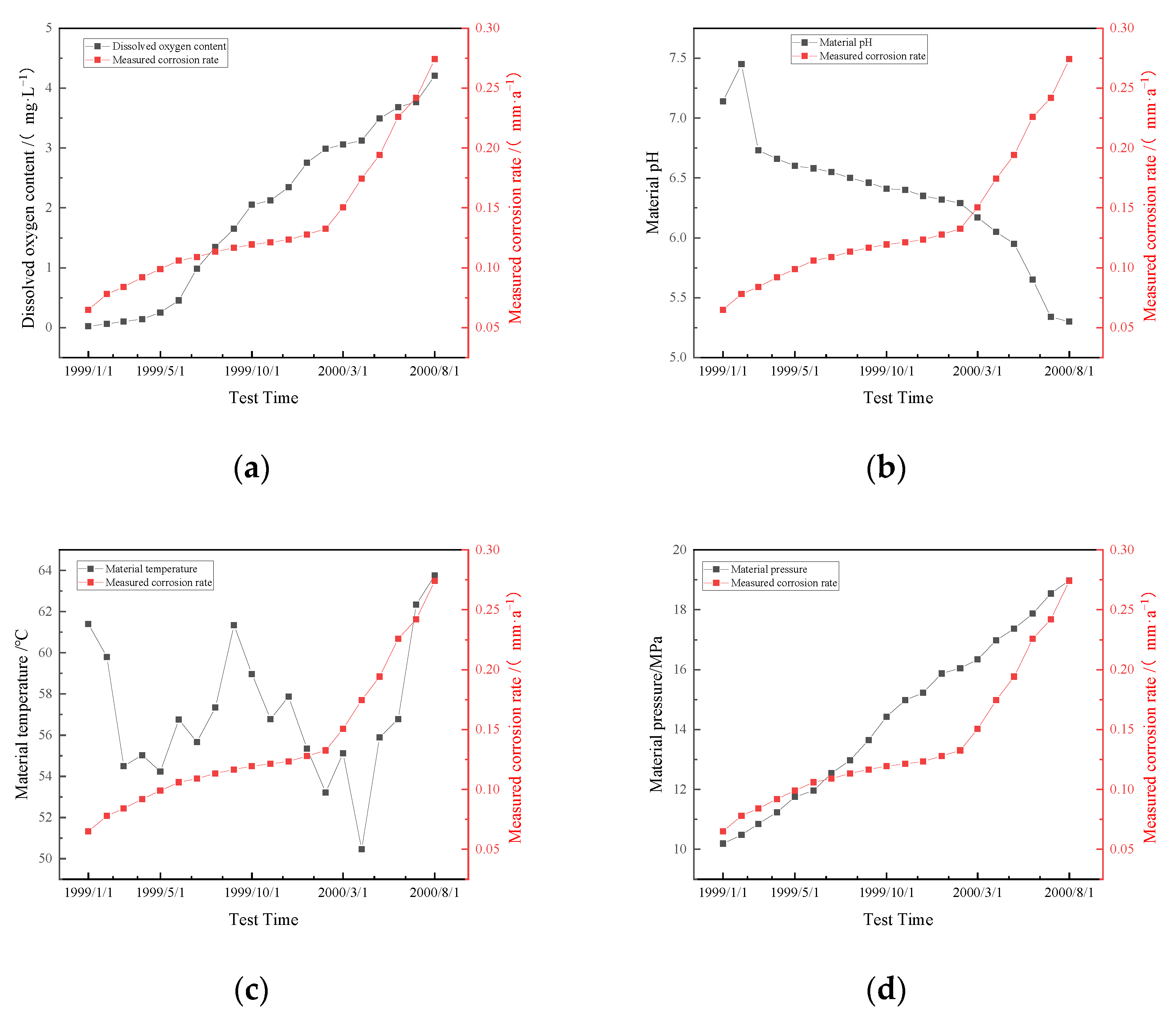
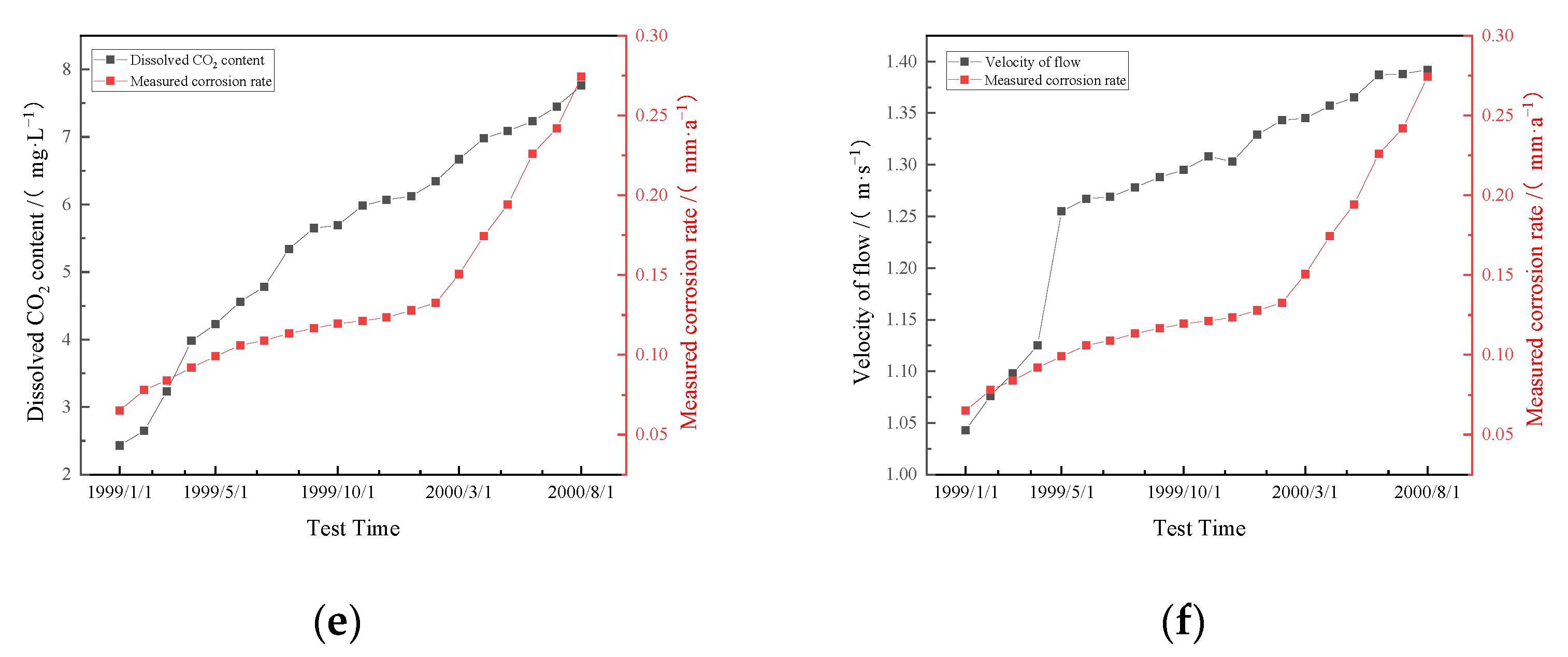
4.1. Data Sources
4.2. The BP Neural Network Modeling Optimization and Prediction
4.3. The Grey Theory Modeling and Prediction
4.4. Modeling Optimization and Prediction of Time Series Prediction Method
4.5. Exponential Smoothing Modeling Optimization and Prediction
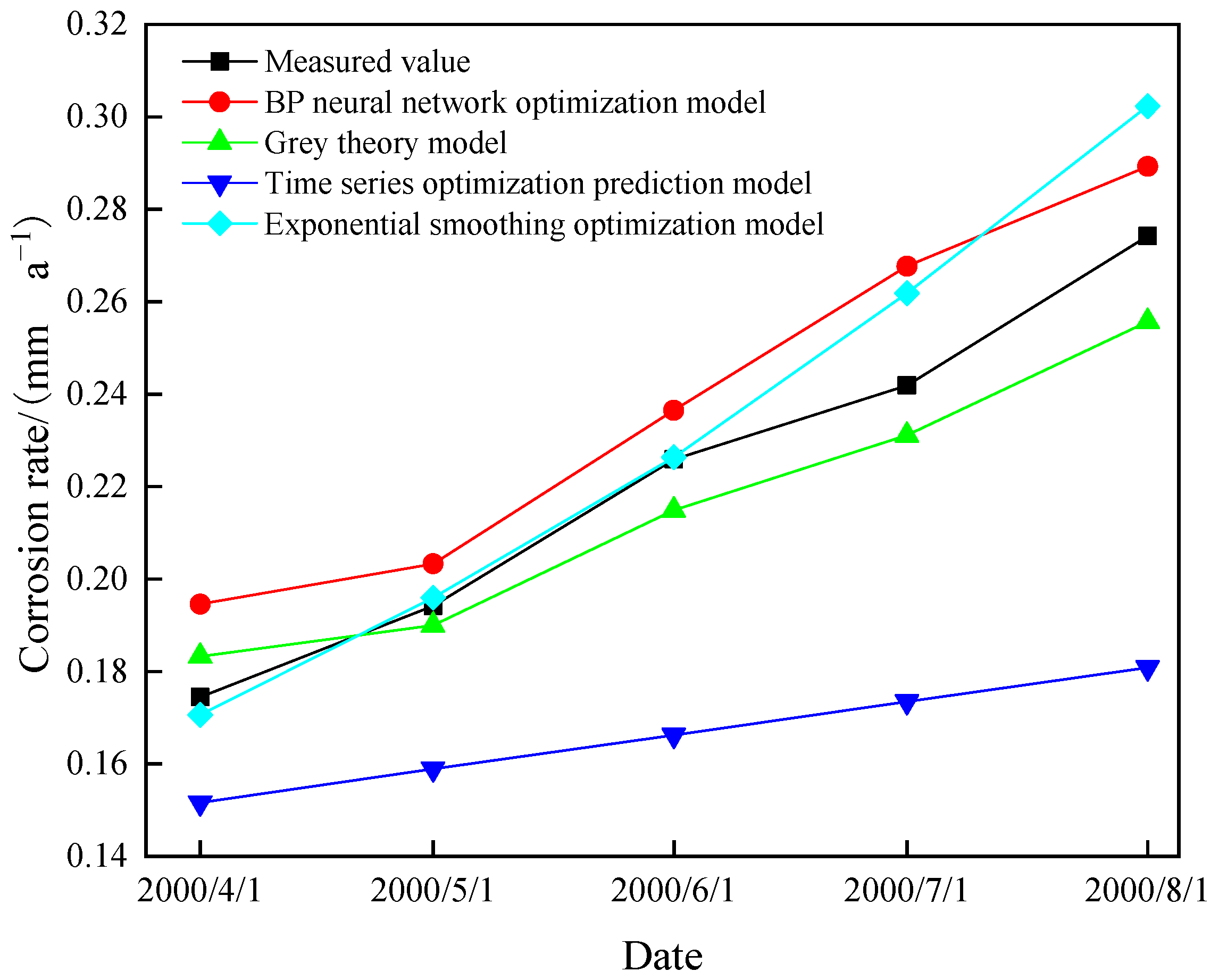
4.6. Comparison and Analysis of Prediction Models
4.7. Summary
5. Conclusions
- (1)
- The existing modeling methods, each with their own benefits and drawbacks, can be used to predict the residual life of corroded pipelines. However, the neural network modeling method can intuitively reflect the relationship between corrosion rate and corrosion influencing factors, and the established model’s basic theory is more reasonable.
- (2)
- The grey theory prediction model is suitable for short-, medium-, and long-term prediction and has the advantages of small samples, lack of sample regularity, low computational workload, and high accuracy. It can fully mine the internal information in a small amount of data and produce a more reasonable prediction from fewer data. Comparative analysis reveals that the grey theory method has good applicability and reliability.
- (3)
- The goal of the time series prediction method is to establish a mathematical model in a way that, given the system’s finite number of operation records (observation data) accurately captures the time series’ dynamic dependencies. The prediction value always remains at its previous level, but it sometimes struggles to accurately predict the future trend. As a result, the accuracy is lower when compared to other prediction models.
- (4)
- The exponential smoothing prediction model is easy to predict, and it only needs to select one model parameter α, and can automatically identify and adjust changes in data patterns. It has a better short-term prediction effect following the gray theory prediction method.
Author Contributions
Funding
Institutional Review Board Statement
Informed Consent Statement
Data Availability Statement
Conflicts of Interest
References
- Zhangx, S.; Xiz, S.; Wangj, Y.; Yangs, T. The prediction on residual life of corroded oil and gas pipeline based on modified GEV distribution. Oil Gas Storage Transp. 2019, 38, 635–641. [Google Scholar]
- Zhangx, S.; Cao, N.; Wangx, W. Residual life prediction of oil and gas pipeline based on Gumbel distribution. China Saf. Sci. J. 2015, 25, 96–101. [Google Scholar]
- Wang, R. Research on Corrosion Failure Prediction of Offshore Oil and Gas Pipeline; XI’AN University of Architecture and Technology: Xi’An, China, 2017; pp. 25–33. [Google Scholar]
- Wang, X.W.; Luo, Z.S.; Wang, R. Study of F-MC method on offshore oil and gas pipelines point corrosion depth forecast. Xi’an University. of Architecture & Technology. Nat. Sci. Ed. 2017, 49, 443–448. [Google Scholar]
- Caleyo, F.; VeLazquez, J.C.; Valor, A.; Hallen, J.M. Probability distribution of pitting corrosion depth and rate in underground pipelines: A Monte Carlo study. Corros. Sci. 2009, 51, 1925–1934. [Google Scholar] [CrossRef]
- Shuai, J. Prediction method for remaining life of corroded Pipeline. J. Univ. Pet. China Ed. Nat. Sci. 2003, 27, 91–93. [Google Scholar]
- Yu, S.R.; Li, J.H.; Li, S.X.; Iang, R. Probability model for the prediction of corrosion remaining life of underground pipelines. China Saf. Sci. J. 2008, 18, 11–15. [Google Scholar]
- Valor, A.; Caleyo, F.; Hallen, J.M.; Velázquez, J.C. Reliability assessment of buried pipelines based on different corrosion rate models. Corros. Sci. 2013, 66, 78–87. [Google Scholar] [CrossRef]
- Hu, Q.F.; Sun, T.; Wang, F.; Ning, C.L.; Zhang, L.B. A method for corrosion depth prediction of gas pipeline based on Bayesian estimation. Oil Gas Storage Transp. 2019, 38, 1219–1226. [Google Scholar]
- Luo, J.H.; Zhao, X.W.; Bai, Z.Q.; Lu, M.X. Prediction of residual life of oil pipe corrosion. China Pet. Mach. 2000, 28, 30–32. [Google Scholar]
- Dann, M.R.; Huyse, L. The effect of inspection sizing uncertainty on the maximum corrosion growth in pipelines. Struct. Saf. 2018, 70, 71–81. [Google Scholar] [CrossRef]
- Yu, X.C.; Zhao, J.Z.; Wu, Y.L.; Hu, Y.Q.; Ji, L.J. Using Gray model to predict corrosion rate variation with time in injecting pipeline. Corros. Prot. 2003, 24, 51–54. [Google Scholar]
- Wang, H.T.; Kong, M.H. Application of cubic exponential smoothing method to pipeline corrosion rate forecasting. Corros. Prot. 2016, 37, 8–11. [Google Scholar]
- Spencer, K.; Kariyawasam, S.; Tetreault, C.; Wharf, J. A practical application to calculating corrosion growth rates by comparing successive ILI runs from different ILI vendors. In Proceedings of the International Pipeline Conference, Calgary, AB, Canada, 27 September–1 October 2010. [Google Scholar]
- Liu, X.N. Reliability prediction of corrosion residual life of steel pressure vessel and pipeline CPM. China Pet. Mach. 2005, 33, 35. [Google Scholar]
- Zhang, X.S.; Cao, X.; Han, W.C.; Chen, P.X. Prediction of submarine pipeline corrosion based on parameter optimized GM-Markov model. Oil Gas Storage Transp. 2020, 39, 953–960. [Google Scholar]
- Xiao, W.W.; Li, J.; Liang, T.T.; Gao, S.Z.; Hu, Y.P.; Wang, Z. Application of BP Neural Network Model in Intelligent Prediction of Pipeline Corrosion Risk. Pet. Tubul. Goods Instrum. 2021, 7, 56–61. [Google Scholar]
- Yao, Q. Research and Implementation of Refinery Equipment Corrosion Prediction Technology; Northeastern University: Shenyang, China, 2014; pp. 29–37. [Google Scholar]
- Ma, M.L. Research on Evaluation of Corrosion Defects and Reinforcing Technology for Qing-Ha Oil Pipeline; Northeast Petroleum University: Daqing, China, 2011. [Google Scholar]
- Wang, S.P. Repairing corrosion defects of sub-sea pipe and the availability of repair method. Oil Gas Storage Transp. 2011, 30, 949–950. [Google Scholar]
- Jiang, Y.W.; Huang, G.Q.; Li, F.F.; Liu, W.H.; Liu, M.; Gai, J.N. Repair technology of anti-corrosion and thermal insulation coating for buried thermal insulation pipeline. Corros. Prot. 2018, 39, 957–961. [Google Scholar]
- Ba, Z.N.; Wang, Z.K.; Liang, J.W.; Han, Y.X.; Wang, M.S. Corrosion risk assessment of gas pipeline network in Suzhou Industrial Park. Oil Gas Storage Transp. 2021, 40, 828–833. [Google Scholar]
- Arruda, M.E.; Li, K.Y. Framework of policies, institutions in place to enable China to meet its soaring oil, gas demand. Oil Gas J. 2004, 102, 20. [Google Scholar]
- Zhang, X.S.; Chang, Y.G. Prediction of external corrosion rate of offshore oil and gas pipelines based on FA-BAS-ELM. China Saf. Sci. J. 2022, 32, 99–106. [Google Scholar]
- Xu, G.X.; Xie, R.J.; Wu, Y.; Yin, Q.S. Prediction Method of Residual Strength of Casing with Different Corrosion Defects. China Pet. Mach. 2019, 47, 122–127. [Google Scholar]

| Serial Number | Test Time | Dissolved Oxygen Content (mg·L−1) | Material pH | Material Temperature °C | Material Pressure MPa | Dissolved CO2 Content (mg·L−1) | Velocity of Flow (m·s−1) | Measured Corrosion Rate (mm·a−1) |
|---|---|---|---|---|---|---|---|---|
| 1 | 1 January 1999 | 0.023 | 7.14 | 61.4 | 10.19 | 2.43 | 1.043 | 0.065 |
| 2 | 1 February 1999 | 0.065 | 7.45 | 59.8 | 10.48 | 2.65 | 1.076 | 0.078 |
| 3 | 1 March 1999 | 0.104 | 6.73 | 54.5 | 10.85 | 3.23 | 1.098 | 0.084 |
| 4 | 1 April 1999 | 0.143 | 6.66 | 55.03 | 11.24 | 3.98 | 1.125 | 0.092 |
| 5 | 1 May 1999 | 0.254 | 6.60 | 54.23 | 11.75 | 4.23 | 1.255 | 0.099 |
| 6 | 1 June 1999 | 0.456 | 6.58 | 56.76 | 11.96 | 4.56 | 1.267 | 0.106 |
| 7 | 1 July 1999 | 0.987 | 6.55 | 55.67 | 12.54 | 4.78 | 1.269 | 0.109 |
| 8 | 1 August 1999 | 1.345 | 6.50 | 57.34 | 12.97 | 5.34 | 1.278 | 0.1134 |
| 9 | 1 September 1999 | 1.654 | 6.46 | 61.34 | 13.65 | 5.65 | 1.288 | 0.1167 |
| 10 | 1 October 1999 | 2.054 | 6.41 | 58.97 | 14.43 | 5.69 | 1.295 | 0.1195 |
| 11 | 1 November 1999 | 2.124 | 6.40 | 56.78 | 14.98 | 5.98 | 1.308 | 0.1213 |
| 12 | 1 December 1999 | 2.345 | 6.35 | 57.87 | 15.23 | 6.07 | 1.303 | 0.1234 |
| 13 | 1 January 2000 | 2.753 | 6.32 | 55.34 | 15.87 | 6.12 | 1.329 | 0.1279 |
| 14 | 1 February 2000 | 2.987 | 6.29 | 53.22 | 16.05 | 6.34 | 1.343 | 0.1326 |
| 15 | 1 March 2000 | 3.057 | 6.17 | 55.12 | 16.34 | 6.67 | 1.345 | 0.1506 |
| 16 | 1 April 2000 | 3.125 | 6.05 | 50.45 | 16.98 | 6.98 | 1.357 | 0.1745 |
| 17 | 1 May 2000 | 3.492 | 5.95 | 55.9 | 17.37 | 7.09 | 1.365 | 0.1942 |
| 18 | 1 June 2000 | 3.682 | 5.65 | 56.78 | 17.87 | 7.23 | 1.387 | 0.2259 |
| 19 | 1 July 2000 | 3.769 | 5.34 | 62.34 | 18.54 | 7.45 | 1.388 | 0.2419 |
| 20 | 1 August 2000 | 4.208 | 5.30 | 63.76 | 18.98 | 7.76 | 1.392 | 0.2742 |
| Training Algorithm | Transfer Function | Trial Calculation Results (mm·a−1) | Mean Square Error between Predicted value and Measured Value | ||||
|---|---|---|---|---|---|---|---|
| 1 April 2000 | 1 May 2000 | 1 June 2000 | 1 July 2000 | 1 August 2000 | |||
| L-M BP | Double tangent S-type | 0.1845 | 0.2042 | 0.2133 | 0.2788 | 0.2932 | 0.000416 |
| S-type | 0.1611 | 0.1783 | 0.2011 | 0.2222 | 0.2488 | 0.000416 | |
| Bayers normalized BP | Double tangent S-type | 0.1533 | 0.1712 | 0.2922 | 0.2356 | 0.2867 | 0.001114 |
| S-type | 0.1595 | 0.1732 | 0.2011 | 0.2207 | 0.2511 | 0.000453 | |
| Training Algorithm | Transfer Function | Trial Calculation Results (mm·a−1) | Mean Square Error between Predicted Value and Measured Value | ||||
|---|---|---|---|---|---|---|---|
| 1 April 2000 | 1 May 2000 | 1 June 2000 | 1 July 2000 | 1 August 2000 | |||
| L-M BP | Double tangent S-type | 0.1443 | 0.1574 | 0.1958 | 0.2114 | 0.2444 | 0.000998 |
| S-type | 0.1946 | 0.2033 | 0.2365 | 0.2677 | 0.2893 | 0.000299 | |
| Bayers normalized BP | Double tangent S-type | 0.1855 | 0.2133 | 0.2484 | 0.2709 | 0.3021 | 0.000522 |
| S-type | 0.1456 | 0.1638 | 0.2099 | 0.2233 | 0.2658 | 0.000486 | |
| N | Parameter | Predictive Value (mm·a−1) | MSE | |||||||
|---|---|---|---|---|---|---|---|---|---|---|
| 1 April 2000 | 1 May 2000 | 1 June 2000 | 1 July 2000 | 1 August 2000 | ||||||
| 3 | 0.137033 | 0.129733 | 0.144333 | 0.007300 | 0.1516 | 0.1595 | 0.1662 | 0.1735 | 0.1808 | 0.003744 |
| 5 | 0.131160 | 0.122540 | 0.139780 | 0.004310 | 0.1441 | 0.1484 | 0.1527 | 0.1570 | 0.1613 | 0.005665 |
| 7 | 0.127429 | 0.115263 | 0.139594 | 0.004055 | 0.1436 | 0.1477 | 0.1518 | 0.1558 | 0.1599 | 0.005819 |
| α | Parameter | Predictive Value (mm·a−1) | MSE | |||||||||
|---|---|---|---|---|---|---|---|---|---|---|---|---|
| 1 April 2000 | 1 May 2000 | 1 June 2000 | 1 July 2000 | 1 August 2000 | ||||||||
| 0.3 | 0.131778 | 0.120023 | 0.110064 | 0.145328 | 0.006742 | 0.000165 | 0.1522 | 0.1595 | 0.1670 | 0.1749 | 0.1832 | 0.003588 |
| 0.5 | 0.139569 | 0.132255 | 0.126884 | 0.148825 | 0.01217 | 0.000971 | 0.1620 | 0.1771 | 0.1941 | 0.2130 | 0.2340 | 0.000783 |
| 0.7 | 0.144631 | 0.139926 | 0.136147 | 0.150261 | 0.017814 | 0.002519 | 0.1706 | 0.1960 | 0.2264 | 0.2618 | 0.3023 | 0.000241 |
| Model | Predictive Value (mm·a−1) | Absolute Error (mm·a−1) | MSE | ||||||||
|---|---|---|---|---|---|---|---|---|---|---|---|
| 1 April 2000 | 1 May 2000 | 1 June 2000 | 1 July 2000 | 1 August 2000 | 1 April 2000 | 1 May 2000 | 1 June 2000 | 1 July 2000 | 1 August 2000 | ||
| BP neural network optimization model | 0.1946 | 0.2033 | 0.2365 | 0.2677 | 0.2893 | 0.0201 | 0.0091 | 0.0106 | 0.0258 | 0.0151 | 0.000299 |
| Grey theory model | 0.1833 | 0.1900 | 0.2149 | 0.2311 | 0.2557 | 0.0088 | 0.0042 | 0.0110 | 0.0108 | 0.0185 | 0.000135 |
| Time series optimization prediction model | 0.1516 | 0.1589 | 0.1662 | 0.1735 | 0.1808 | 0.0229 | 0.0353 | 0.0597 | 0.0684 | 0.0934 | 0.003744 |
| Exponential smoothing optimization model | 0.1706 | 0.1960 | 0.2264 | 0.2618 | 0.3023 | 0.0039 | 0.0018 | 0.0005 | 0.0199 | 0.0281 | 0.000241 |
| Measured value/(mm·a−1) | 0.1745 | 0.1942 | 0.2259 | 0.2419 | 0.2742 | / | / | / | / | / | / |
Publisher’s Note: MDPI stays neutral with regard to jurisdictional claims in published maps and institutional affiliations. |
© 2022 by the authors. Licensee MDPI, Basel, Switzerland. This article is an open access article distributed under the terms and conditions of the Creative Commons Attribution (CC BY) license (https://creativecommons.org/licenses/by/4.0/).
Share and Cite
Zuo, L.; Zeng, C.; Hu, X.; Du, S.; Zhao, Y.; Fei, F. Evaluation of Corrosion Residual Life Prediction Methods for Metal Pipelines. Materials 2022, 15, 5624. https://doi.org/10.3390/ma15165624
Zuo L, Zeng C, Hu X, Du S, Zhao Y, Fei F. Evaluation of Corrosion Residual Life Prediction Methods for Metal Pipelines. Materials. 2022; 15(16):5624. https://doi.org/10.3390/ma15165624
Chicago/Turabian StyleZuo, Lili, Chunlei Zeng, Xingqiao Hu, Shengjie Du, Yun Zhao, and Fan Fei. 2022. "Evaluation of Corrosion Residual Life Prediction Methods for Metal Pipelines" Materials 15, no. 16: 5624. https://doi.org/10.3390/ma15165624
APA StyleZuo, L., Zeng, C., Hu, X., Du, S., Zhao, Y., & Fei, F. (2022). Evaluation of Corrosion Residual Life Prediction Methods for Metal Pipelines. Materials, 15(16), 5624. https://doi.org/10.3390/ma15165624