Research on Hyperparameter Optimization of Concrete Slump Prediction Model Based on Response Surface Method
Abstract
:1. Introduction
2. Establishment of a Concrete Slump Model Based on BP Neural Network
2.1. Introduction to BP Neural Network
2.2. Samples and Network Input and Output
2.3. Network Data Preprocessing
- (1)
- (2)
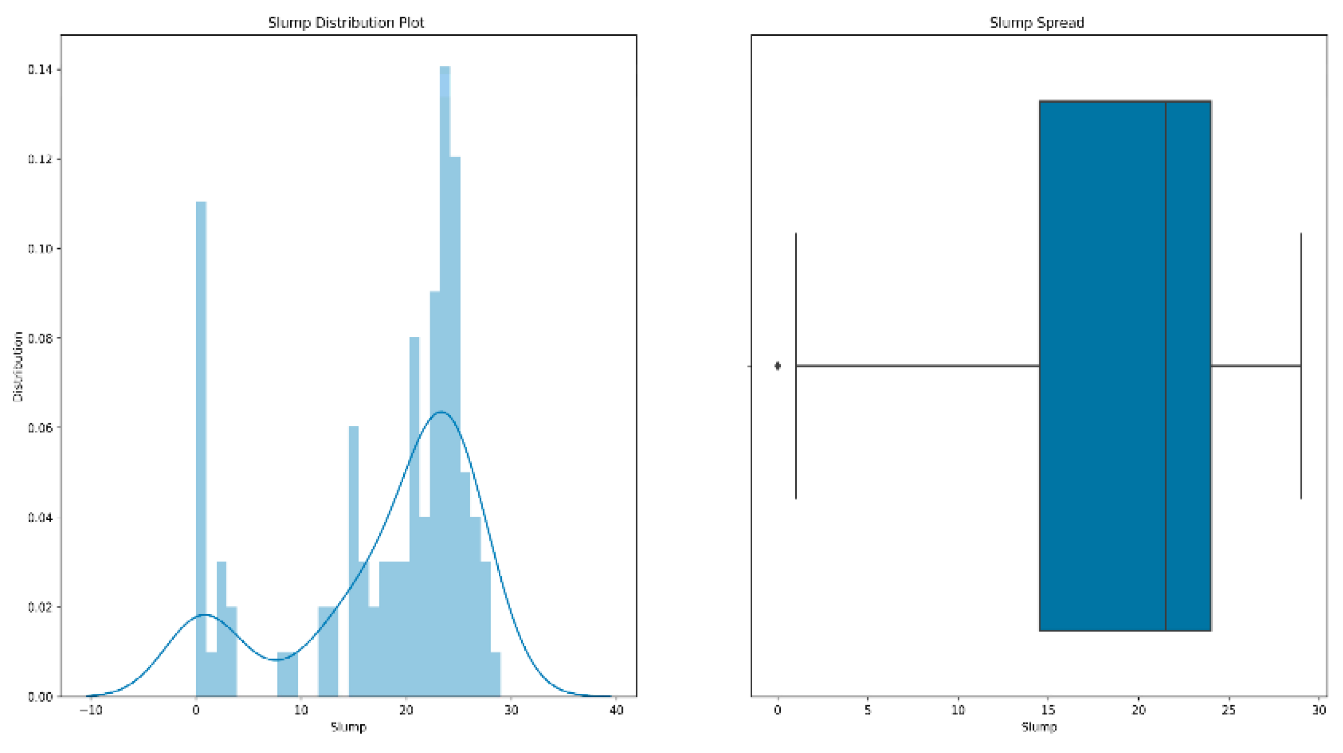
- Outlier processing: It is inevitable that we will have a few data points that are significantly different from other observations during training. A data point is considered to be an outlier [39] if it lies 1.5 times the interquartile range below the first quartile or above the third quartile. The existence of outliers will have a serious impact on the prediction results of the model. Therefore, our processing of outliers [40,41] is generally to delete them. Figure 5 is a box diagram of the model’s slump distribution.
- (3)
- Split the dataset as follows: the training set accounts for 70%, the test set accounts for 30% and the feature variables are kept separate from the test set and training set data.
- (4)
- Standardized data: There are three main methods for data standardization, namely minimum–maximum standardization, z-score standardization and decimal standardization. This paper adopts the z-score method, also called standard deviation normalization, the mean value of the data processed by it is 0 and the variance is 1. It is currently the most commonly used standardization method. The formula is as follows:where is the mean value of the corresponding feature and σ is the standard deviation.
2.4. Model Parameter Selection
3. Research on Two-Layer Neural Network
3.1. Single Factor Design Experiment of Two-Layer Neural Network
3.2. Response Surface Method Test of Two-Layer Neural Network
3.2.1. Model Establishment and Significance Test of a Two-Layer Neural Network
3.2.2. Response Surface Method Analysis of Two-Layer Neural Network
3.2.3. Analysis of Slump Influencing Factors Based on Two-Layer Neural Network
4. Research on Three-Layer Neural Network
4.1. Single Factor Design Experiment of Three-Layer Neural Network
4.2. Response Surface Method Test of Three-Layer Neural Network
4.2.1. Model Establishment and Significance Test of Three-Layer Neural Network
4.2.2. Response Surface Method Analysis of Three-Layer Neural Network
4.2.3. Analysis of Slump Influencing Factors Based on Three-Layer Neural Network
5. Conclusions and Analysis
- (1)
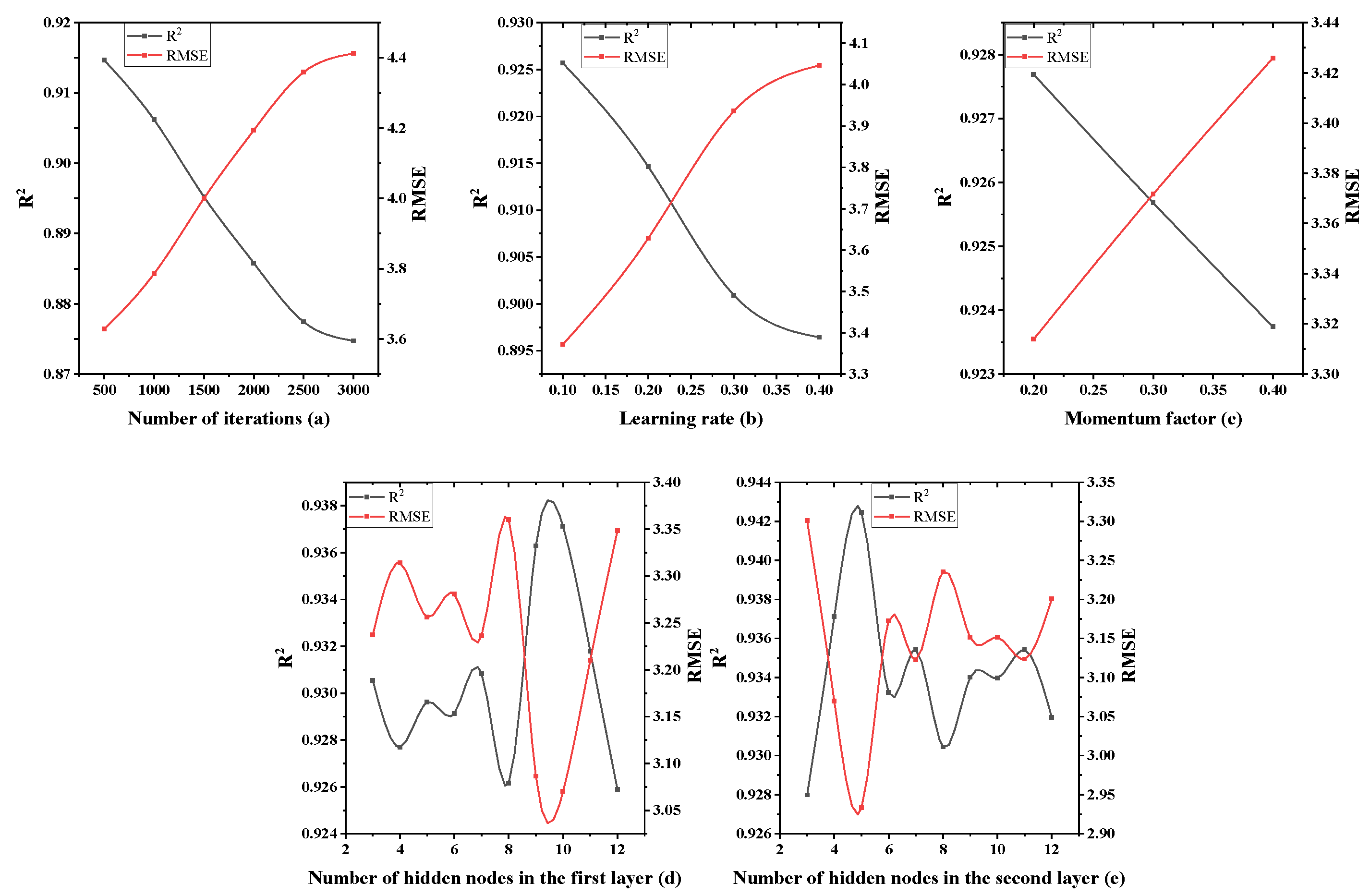
- In the two-layer neural network model, the learning rate has the most significant impact on the entire model and the change of other parameters has a weaker effect on the network model. The reason for this phenomenon is that as the learning rate increases, the network weight value is updated too much, the swing amplitude exceeds the training range of the model performance and, finally, the system prediction deviation becomes too large. It can also be seen that the network performance of the two-layer neural network is relatively stable. A two-layer neural network constructed by optimization parameters was used to evaluate the test set, and the results are R2 = 0.927 and RMSE = 3.373. At the same time, the unoptimized two-layer neural network was evaluated on the test set, and the result was only R2 = 0.91623.
- (2)
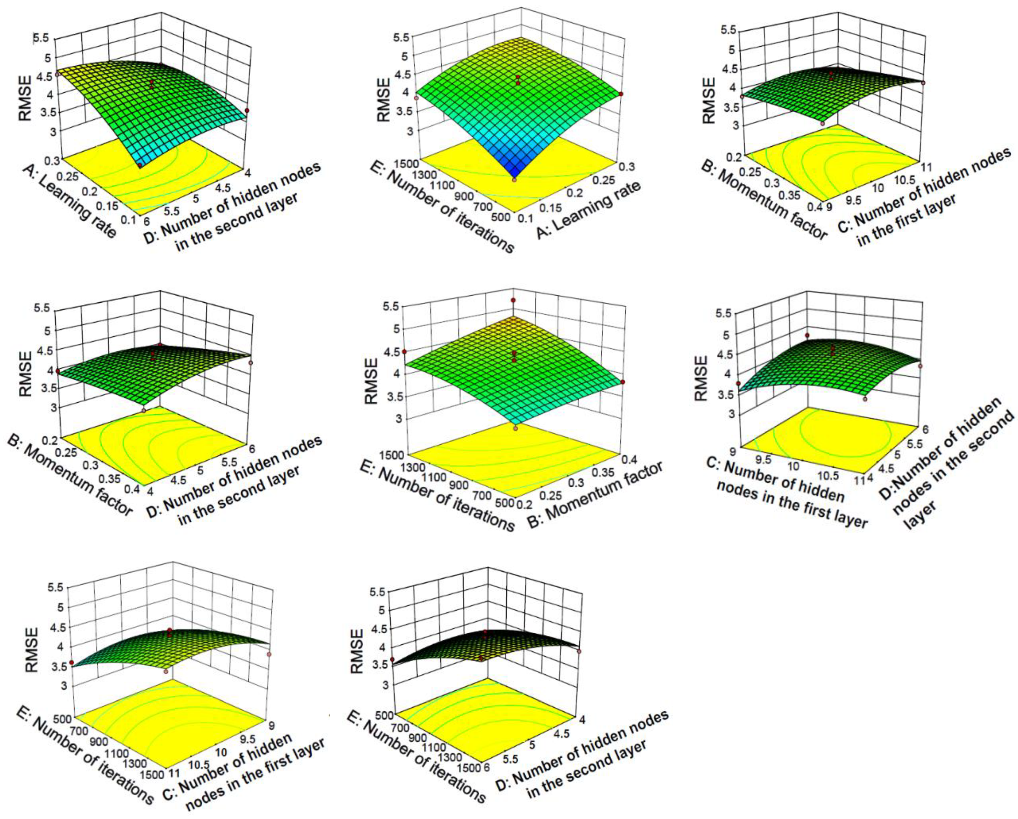
- In the three-layer neural network model, the interaction between the parameters is relatively strong and compared with the two-layer neural network, its predictive ability is stronger. A three-layer neural network constructed by optimization parameters was used to evaluate the test set, and the results are R2 = 0.955 and RMSE = 2.781. At the same time, the unoptimized three-layer neural network was evaluated on the test set, and the result was only R2 = 0.94246. From the response surface graph, the coefficient of determination and the root mean square error, it can be seen that the three-layer neural network is more stable and more accurate.
- (3)
- Interestingly, it can be seen from Figure 8 and Figure 11 that the four main factors affecting the slump are flow, water, coarse aggregate and fine aggregate, which also shows that the two-layer neural network and the three-layer neural network have the same law in evaluating the factors affecting the slump. Of course, there are differences between the two-layer neural network and three-layer neural network in the prediction of influencing factors of the slump. Two-layer neural network results show that coarse aggregate is the second factor affecting slump, while three-layer neural network results indicate that water is the second factor affecting slump. In addition, the influence factor of flow evaluated by the two-layer neural network is even more than 0.9, while the influence factor of each variable evaluated by the three-layer neural network on the slump is relatively reasonable. Therefore, the prediction performance of three-layer neural network is better than that of two-layer neural network.
- (1)
- The basic data of concrete slump in this experiment are too small, which, more or less, affects the accuracy of the conclusion. Based on this, it could be considered to further expand the data to achieve a more accurate and reliable effect.
- (2)
- The BP neural network used in this paper has a similar “black box” effect, and many model parameters are not interpretable. The next step also requires the use of state-of-the-art deep learning algorithms (e.g., interpretable neural networks) for concrete slump prediction.
Author Contributions
Funding
Institutional Review Board Statement
Informed Consent Statement
Data Availability Statement
Conflicts of Interest
References
- Xu, G.Q.; Su, Y.P.; Han, T.L. Prediction model of compressive strength of green concrete based on BP neural network. Concrete 2013, 2, 33–35. [Google Scholar]
- Gambhir, M.L. Concrete Technology: Theory and Practice; Tata McGraw-Hill Education: Noida, India, 2013. [Google Scholar]
- Ramezani, M.; Kim, Y.H.; Hasanzadeh, B.; Sun, Z. Influence of carbon nanotubes on SCC flowability. In Proceedings of the 8th International RILEM Symposium on Self-Compacting Concrete, Washington DC, USA, 15–18 May 2016; pp. 97–406. [Google Scholar]
- Ramezani, M.; Dehghani, A.; Sherif, M.M. Carbon nanotube reinforced cementitious composites: A comprehensive review. Constr. Build. Mater. 2022, 315, 125100. [Google Scholar] [CrossRef]
- Sun, Y.L.; Liao, X.H.; Li, Y. Slump prediction of recycled concrete. Concrete 2013, 6, 81–83. [Google Scholar]
- Qi, C.Y. Study on Slump Loss Mechanism of Concrete and Slump-Preserving Materials; Wuhan University of Technology: Wuhan, China, 2015. [Google Scholar]
- Li, Y.L. Building Materials; China Construction Industry Press: Beijing, China, 1993. [Google Scholar]
- Ge, P.; Sun, Z.Q. Neural Network Theory and Implementation of MATLABR2007; Electronic Industry Press: Beijing, China, 2007. [Google Scholar]
- Lei, Y.J. MATLAB Genetic Algorithm Toolbox and Application; Xidian University Press: Xi’an, China, 2005. [Google Scholar]
- Hu, X.; Li, B.; Mo, Y.; Alselwi, O. Progress in artificial intelligence-based prediction of concrete performance. J. Adv. Concr. Technol. 2021, 19, 924–936. [Google Scholar] [CrossRef]
- Shariati, M.; Mafipour, M.S.; Mehrabi, P.; Ahmadi, M.; Wakil, K.; Trung, N.T.; Toghroli, A. Prediction of concrete strength in presence of furnace slag and fly ash using Hybrid ANN-GA (Artificial Neural Network-Genetic Algorithm). Smart Struct. Syst. 2020, 25, 183–195. [Google Scholar]
- Yeh, I.C. Design of high-performance concrete mixture using neural networks and nonlinear programming. J. Comput. Civ. Eng. 1999, 13, 36–42. [Google Scholar] [CrossRef]
- Yeh, I.C. Simulation of concrete slump using neural networks. Constr. Mater. 2009, 162, 11–18. [Google Scholar] [CrossRef]
- Koneru, V.S.; Ghorpade, V.G. Assessment of strength characteristics for experimental based workable self-compacting concrete using artificial neural network. Mater. Today Proc. 2020, 26, 1238–1244. [Google Scholar] [CrossRef]
- Duan, Z.H.; Kou, S.C.; Poon, C.S. Prediction of compressive strength of recycled aggregate concrete using artificial neural networks. Constr. Build. Mater. 2013, 40, 1200–1206. [Google Scholar] [CrossRef]
- Ji, T.; Lin, T.; Lin, X. A concrete mix proportion design algorithm based on artificial neural networks. Cem. Concr. Res. 2006, 36, 1399–1408. [Google Scholar] [CrossRef]
- Demir, F. Prediction of elastic modulus of normal and high strength concrete by artificial neural networks. Constr. Build. Mater. 2008, 22, 1428–1435. [Google Scholar] [CrossRef]
- Chandwani, V.; Agrawal, V.; Nagar, R. Modeling slump of ready mix concrete using genetic algorithms assisted training of Artificial Neural Networks. Expert Syst. Appl. 2015, 42, 885–893. [Google Scholar] [CrossRef]
- Li, D.H.; Gao, Q.; Xia, X.; Zhang, J.W. Prediction of comprehensive performance of concrete based on BP neural network. Mater. Guide 2019, 33, 317–320. [Google Scholar]
- Yeh, I.C. Analysis of strength of concrete using design of experiments and neural networks. J. Mater. Civ. Eng. 2006, 18, 597–604. [Google Scholar] [CrossRef]
- Jain, A.; Jha, S.K.; Misra, S. Modeling and analysis of concrete slump using artificial neural networks. J. Mater. Civ. Eng. 2008, 20, 628–633. [Google Scholar] [CrossRef]
- Wang, J.Z.; Lu, Z.C. Optimal design of mix ratio of high-strength concrete based on genetic algorithm. Concr. Cem. Prod. 2004, 6, 19–22. [Google Scholar]
- Lim, C.H.; Yoon, Y.S.; Kim, J.H. Genetic algorithm in mix proportioning of high-performance concrete. Cem. Concr. Res. 2004, 34, 409–420. [Google Scholar] [CrossRef]
- Liu, C.L.; Li, G.F. Optimal design of mix ratio of fly ash high performance concrete based on genetic algorithm. J. Lanzhou Univ. Technol. 2006, 32, 133–135. [Google Scholar]
- Yeh, I.C. Computer-aided design for optimum concrete mixtures. Cem. Concr. Compos. 2007, 29, 193–202. [Google Scholar] [CrossRef]
- Li, Y. Design and Optimization of Classifier Based on Neural Network; Anhui Agricultural University: Hefei, China, 2013. [Google Scholar]
- Gao, P.Y. Research on BP Neural Network Classifier Optimization Technology; Huazhong University of Science and Technology: Wuhan, China, 2012. [Google Scholar]
- Lei, W. Principle, Classification and Application of Artificial Neural Network. Sci. Technol. Inf. 2014, 3, 240–241. [Google Scholar]
- Jiao, Z.Q. Principle and Application of BP Artificial Neural Network. Technol. Wind. 2010, 12, 200–201. [Google Scholar]
- Ma, Q.M. Research on Email Classification Algorithm of BP Neural Network Based on Perceptron Optimization; University of Electronic Science and Technology of China: Chengdu, China, 2011. [Google Scholar]
- Yeh, I.C. Exploring concrete slump model using artificial neural networks. J. Comput. Civ. Eng. 2006, 20, 217–221. [Google Scholar] [CrossRef]
- Wang, B.B.; Zhao, T.L. A study on prediction of wind power based on improved BP neural network based on genetic algorithm. Electrical 2019, 12, 16–21. [Google Scholar]
- Gulcehre, C.; Moczulski, M.; Denil, M.; Bengio, Y. Noisy activation functions. Int. Conf. Mach. Learn. 2016, 48, 3059–3068. [Google Scholar]
- Li, Z.X.; Wei, Z.B.; Shen, J.L. Coral concrete compressive strength prediction model based on BP neural network. Concrete 2016, 1, 64–69. [Google Scholar]
- Yeh, I.C. Modeling slump flow of concrete using second-order regressions and artificial neural networks. Cem. Concr. Compos. 2007, 29, 474–480. [Google Scholar] [CrossRef]
- Shen, J.R.; Xu, Q.J. Prediction of Shear Strength of Roller Compacted Concrete Dam Layers Based on Artificial Neural Network and Fuzzy Logic System. J. Tsinghua Univ. 2019, 59, 345–353. [Google Scholar]
- Ramezani, M.; Kim, Y.H.; Sun, Z. Probabilistic model for flexural strength of carbon nanotube reinforced cement-based materials. Compos. Struct. 2020, 253, 112748. [Google Scholar] [CrossRef]
- Ramezani, M.; Kim, Y.H.; Sun, Z. Elastic modulus formulation of cementitious materials incorporating carbon nanotubes: Probabilistic approach. Constr. Build. Mater. 2021, 274, 122092. [Google Scholar] [CrossRef]
- Ramezani, M.; Kim, Y.H.; Sun, Z. Mechanical properties of carbon-nanotube-reinforced cementitious materials: Database and statistical analysis. Mag. Concr. Res. 2020, 72, 1047–1071. [Google Scholar] [CrossRef]
- Yu, C.; Weng, S.Y. Outlier detection and variable selection of mixed regression model based on non-convex penalty likelihood method. Stat. Decis. 2020, 36, 5–10. [Google Scholar]
- Zhao, H.; Shao, S.H.; Xie, D.P. Methods of processing outliers in analysis data. J. Zhoukou Norm. Univ. 2004, 5, 70–71+115. [Google Scholar]
- Fu, P.P.; Si, Q.; Wang, S.X. Hyperparameter optimization of machine learning algorithms: Theory and practice. Comput. Program. Ski. Maint. 2020, 12, 116–117+146. [Google Scholar]
- Kumar, M.; Mishra, S.K. Jaya based functional link multilayer perceptron adaptive filter for Poisson noise suppression from X-ray images. Multimed. Tools Appl. 2018, 77, 24405–24425. [Google Scholar] [CrossRef]
- Hammoudi, A.; Moussaceb, K.; Belebchouche, C.; Dahmoune, F. Comparison of artificial neural network (ANN) and response surface methodology (RSM) prediction in compressive strength of recycled concrete aggregates. Constr. Build. Mater. 2019, 209, 425–436. [Google Scholar] [CrossRef]

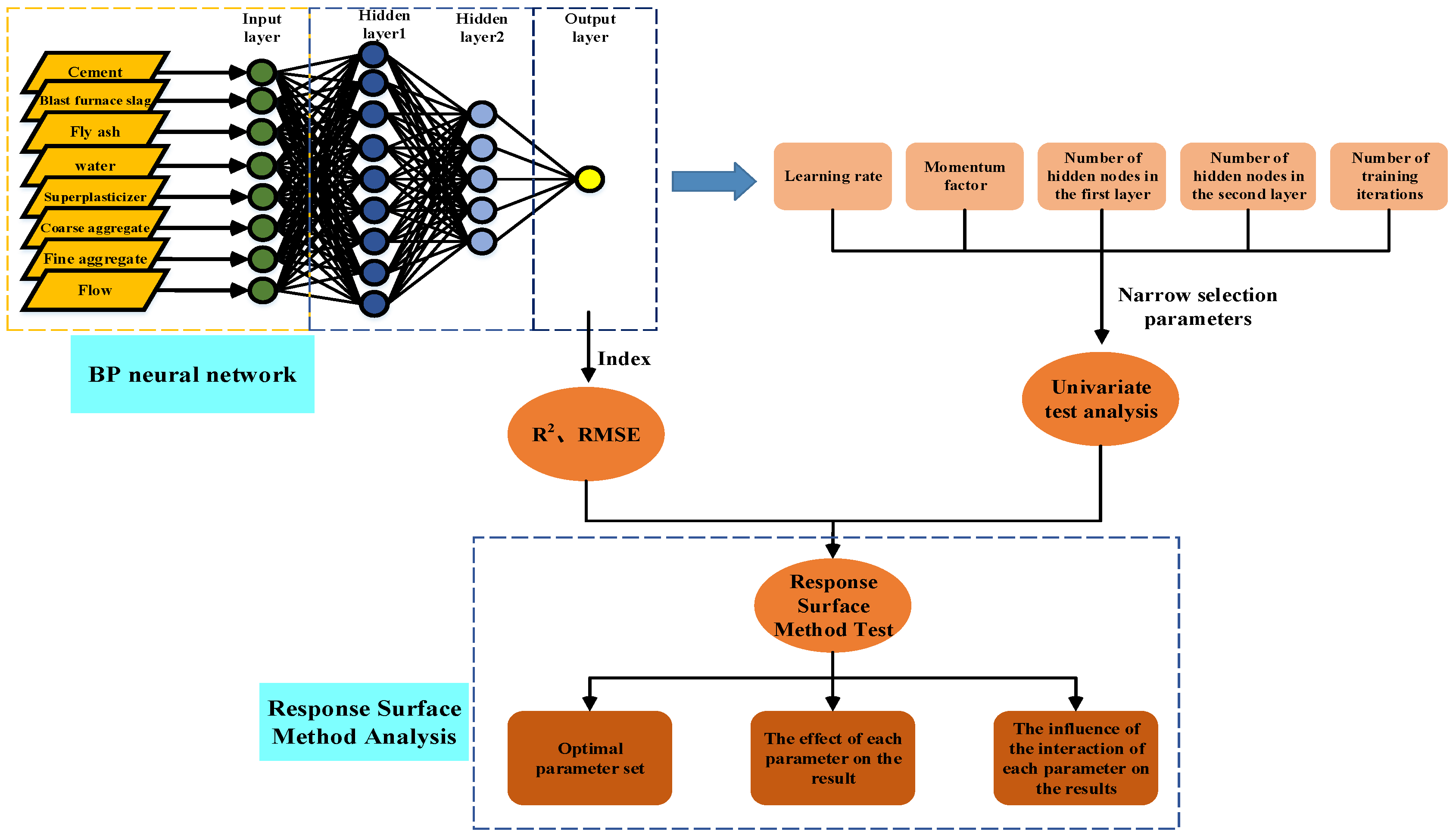

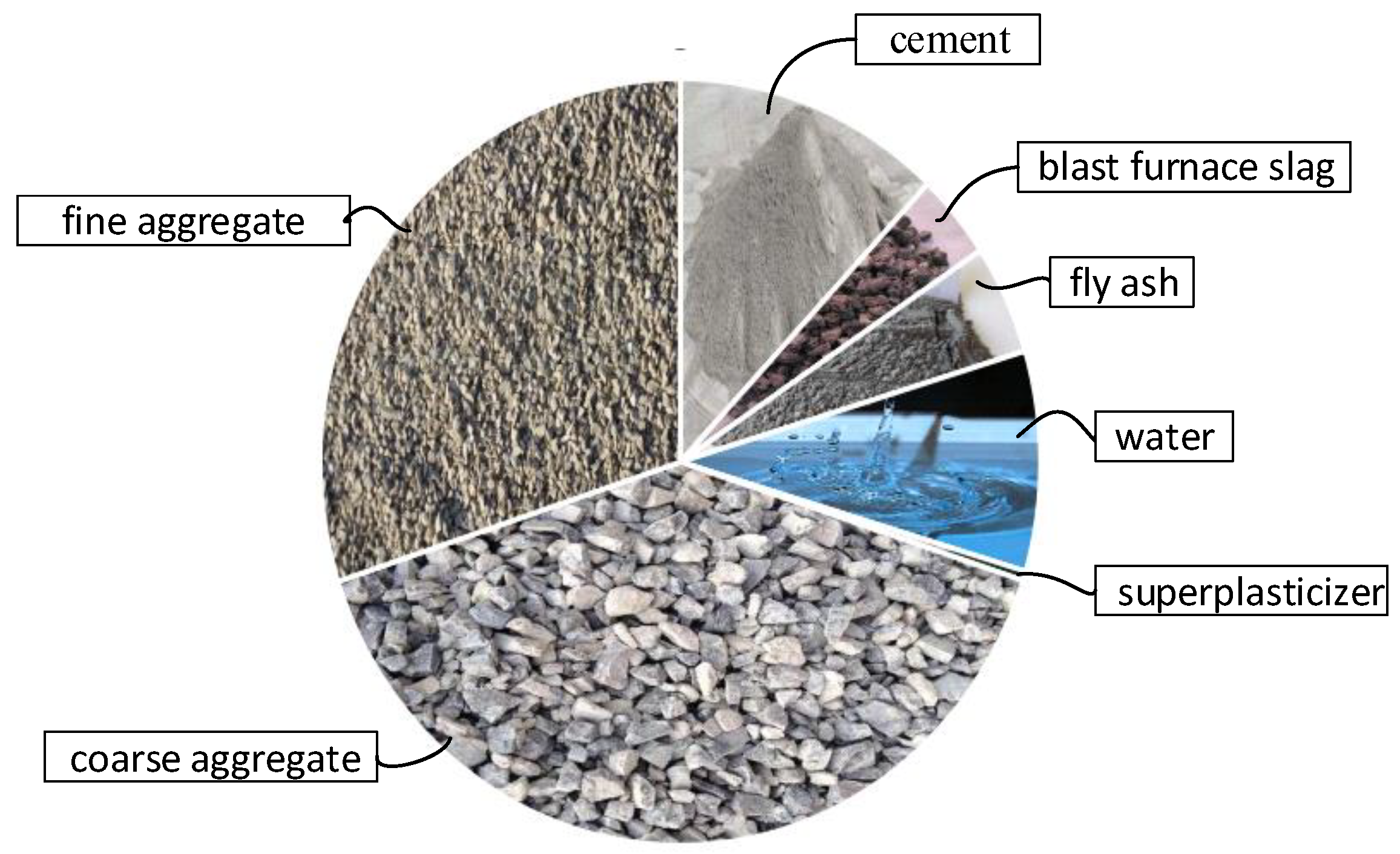
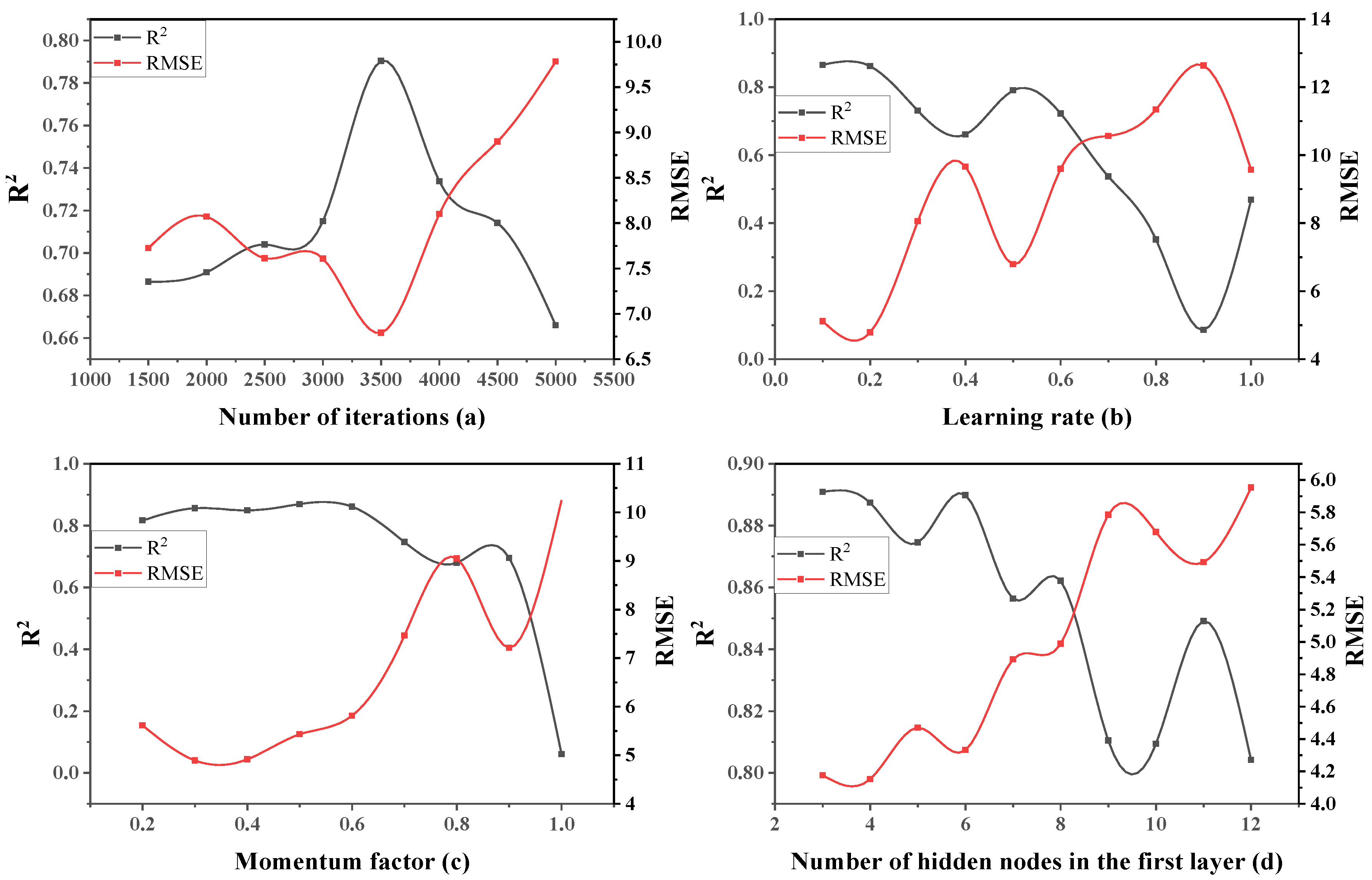




| Mix Ratio | Cement (kg/m3) | Blast Furnace Slag (kg/m3) | Fly Ash (kg/m3) | Water (kg/m3) | Superplasticizer (kg/m3) | Coarse Aggregate (kg/m3) | Fine Aggregate (kg/m3) | Flow (mm) | Slump (cm) |
|---|---|---|---|---|---|---|---|---|---|
| C-1 | 273 | 82 | 105 | 210 | 9 | 904 | 680 | 62 | 23 |
| C-2 | 162 | 148 | 190 | 179 | 19 | 838 | 741 | 20 | 1 |
| C-3 | 147 | 89 | 115 | 202 | 9 | 860 | 829 | 55 | 23 |
| C-4 | 145 | 0 | 227 | 240 | 6 | 750 | 853 | 58.5 | 14.5 |
| C-5 | 148 | 109 | 139 | 193 | 7 | 768 | 902 | 58 | 23.75 |
| C-6 | 374 | 0 | 0 | 190 | 7 | 1013 | 730 | 42.5 | 14.5 |
| ⋮ | ⋮ | ⋮ | ⋮ | ⋮ | ⋮ | ⋮ | ⋮ | ⋮ | ⋮ |
| C-102 | 150.3 | 111.4 | 238.8 | 167.3 | 6.5 | 999.5 | 670.5 | 36.5 | 14.5 |
| C-103 | 303.8 | 0.2 | 239.8 | 236.4 | 8.3 | 780.1 | 715.3 | 78 | 25 |
| Serial Number | Cement | Slag | Fly Ash | Water | SP | Coarse Aggr | Fine Aggr | Flow |
|---|---|---|---|---|---|---|---|---|
| 98 | 0.148284 | 0.417310 | 1.075807 | −1.460561 | −0.168038 | 0.820139 | −1.569612 | −1.711562 |
| 81 | −1.206461 | −1.099031 | 0.921458 | 0.504346 | −1.210391 | 1.567436 | −0.873459 | 0.885664 |
| 75 | −1.09526 | 0.553305 | −0.112678 | −0.243228 | −0.800895 | 0.123258 | 0.676771 | 0.561011 |
| 53 | 0.908293 | −1.299623 | −0.077259 | 1.019566 | 0.688181 | 0.347335 | −0.934695 | 0.767608 |
| 46 | 0.545192 | 0.264316 | −0.362010 | 0.463936 | 0.315912 | 0.022423 | −0.950810 | 0.885664 |
| Parameter Type | Parameter Selection Range | |||||||||
|---|---|---|---|---|---|---|---|---|---|---|
| learning rate | 0.1 | 0.2 | 0.3 | 0.4 | 0.5 | 0.6 | 0.7 | 0.8 | 0.9 | 1.0 |
| momentum factor | 0.2 | 0.3 | 0.4 | 0.5 | 0.6 | 0.7 | 0.8 | 0.9 | 1.0 | - |
| number of hidden nodes in the first layer | 3 | 4 | 5 | 6 | 7 | 8 | 9 | 10 | 11 | 12 |
| number of hidden nodes in the second layer | 3 | 4 | 5 | 6 | 7 | 8 | 9 | 10 | 11 | 12 |
| number of training iterations | 500 | 1000 | 1500 | 2000 | 2500 | 3000 | 3500 | 4000 | 4500 | 5000 |
| Momentum Factor | Learning Rate | Number of Hidden Nodes | Number of Iterations | R2 | RMSE |
|---|---|---|---|---|---|
| 0.2 | 0.1 | 3 | 2500 | 0.862279 | 3.2887 |
| 0.2 | 0.1 | 4 | 2500 | 0.842614 | 3.4821 |
| 0.2 | 0.1 | 5 | 2500 | 0.807051 | 4.0261 |
| 0.2 | 0.1 | 6 | 2500 | 0.763754 | 4.5256 |
| 0.2 | 0.1 | 7 | 2500 | 0.77447 | 4.4553 |
| 0.2 | 0.1 | 8 | 2500 | 0.804214 | 4.1351 |
| 0.2 | 0.1 | 9 | 2500 | 0.771077 | 4.5278 |
| 0.2 | 0.1 | 10 | 2500 | 0.759843 | 4.2585 |
| 0.2 | 0.1 | 11 | 2500 | 0.73613 | 4.66 |
| 0.2 | 0.1 | 12 | 2500 | 0.847652 | 4.8972 |
| Serial Number | LR | MF | HU | Epochs | R2 | RMSE |
|---|---|---|---|---|---|---|
| 1 | 0.5 | 0.6 | 7 | 3500 | 0.79033 | 6.791 |
| 2 | 0.5 | 0.6 | 7 | 500 | 0.74777 | 7.00612 |
| 3 | 0.5 | 0.6 | 7 | 3000 | 0.71497 | 7.60734 |
| 4 | 0.5 | 0.6 | 7 | 2500 | 0.7039 | 7.61213 |
| 5 | 0.5 | 0.6 | 7 | 1500 | 0.6864 | 7.72466 |
| 6 | 0.5 | 0.6 | 7 | 1000 | 0.65952 | 8.06336 |
| 7 | 0.5 | 0.6 | 7 | 2000 | 0.69084 | 8.07128 |
| 8 | 0.5 | 0.6 | 7 | 4000 | 0.73372 | 8.10192 |
| 9 | 0.5 | 0.6 | 7 | 4500 | 0.71407 | 8.89968 |
| 10 | 0.5 | 0.6 | 7 | 5000 | 0.66591 | 9.78058 |
| Hidden Layers | Number of Hidden Nodes | Learning Rate | Momentum Factor | Number of Training Iterations |
|---|---|---|---|---|
| 1 | 4 | 0.2 | 0.3 | 3500 |
| Factor | −1 | 0 | 1 |
|---|---|---|---|
| Learning rate | 0.1 | 0.2 | 0.3 |
| Momentum factor | 0.2 | 0.3 | 0.4 |
| Number of hidden nodes | 3 | 4 | 5 |
| Number of iterations | 2500 | 3500 | 4500 |
| Serial Number | X1 | X2 | X3 | X4 | Y1 | Y2 |
|---|---|---|---|---|---|---|
| 1 | 0.1 | 0.2 | 4 | 3500 | 0.91166 | 3.63823 |
| 2 | 0.3 | 0.2 | 4 | 3500 | 0.82037 | 5.58347 |
| 3 | 0.1 | 0.4 | 4 | 3500 | 0.90076 | 3.90087 |
| 4 | 0.3 | 0.4 | 4 | 3500 | 0.84698 | 4.92102 |
| 5 | 0.2 | 0.3 | 3 | 2500 | 0.89911 | 4.01026 |
| 6 | 0.2 | 0.3 | 5 | 2500 | 0.87238 | 4.529 |
| 7 | 0.2 | 0.3 | 3 | 4500 | 0.88607 | 4.27762 |
| 8 | 0.2 | 0.3 | 5 | 4500 | 0.87633 | 4.43749 |
| 9 | 0.1 | 0.3 | 4 | 2500 | 0.92411 | 3.40633 |
| ⋮ | ⋮ | ⋮ | ⋮ | ⋮ | ⋮ | ⋮ |
| 28 | 0.2 | 0.3 | 4 | 3500 | 0.88984 | 4.19149 |
| 29 | 0.2 | 0.3 | 4 | 3500 | 0.87953 | 4.07428 |
| Source | Sum of Squares | df | Mean Square | F Value | p-Value Prob > F | Significance |
|---|---|---|---|---|---|---|
| Model | 0.012 | 14 | 8.607 × 10⁻⁴ | 8.41 | 0.0001 | significant |
| X1 | 9.547 × 10⁻³ | 1 | 9.547 × 10⁻³ | 93.28 | <0.0001 | ** |
| X2 | 2.846 × 10⁻⁵ | 1 | 2.846 × 10⁻⁵ | 0.28 | 0.6062 | |
| X3 | 1.103 × 10⁻³ | 1 | 1.103 × 10⁻³ | 10.77 | 0.0055 | ** |
| X4 | 2.629 × 10⁻⁴ | 1 | 2.629 × 10⁻⁴ | 2.57 | 0.1313 | |
| X1 × 2 | 3.518 × 10⁻⁴ | 1 | 3.518 × 10⁻⁴ | 3.44 | 0.085 | |
| X1 × 3 | 7.293 × 10⁻⁵ | 1 | 7.293 × 10⁻⁵ | 0.71 | 0.4128 | |
| X1 × 4 | 8.791 × 10⁻⁶ | 1 | 8.791 × 10⁻⁶ | 0.086 | 0.7738 | |
| X2 × 3 | 3.686 × 10⁻⁶ | 1 | 3.686 × 10⁻⁶ | 0.036 | 0.8522 | |
| X2 × 4 | 9.517 × 10⁻⁶ | 1 | 9.517 × 10⁻⁶ | 0.093 | 0.7649 | |
| X3 × 4 | 7.217 × 10⁻⁵ | 1 | 7.217 × 10⁻⁵ | 0.71 | 0.4152 | |
| X12 | 2.406 × 10⁻⁵ | 1 | 2.406 × 10⁻⁵ | 0.24 | 0.6353 | |
| X22 | 2.446 × 10⁻⁴ | 1 | 2.446 × 10⁻⁴ | 2.39 | 0.1444 | |
| X32 | 5.259 × 10⁻⁷ | 1 | 5.259 × 10⁻⁷ | 5.139 × 10⁻³ | 0.9439 | |
| X42 | 2.143 × 10⁻⁴ | 1 | 2.143 × 10⁻⁴ | 2.09 | 0.1699 | |
| Residual | 1.433 × 10⁻³ | 14 | 1.024 × 10⁻⁴ | |||
| Lack of Fit | 1.335 × 10⁻³ | 10 | 1.335 × 10⁻⁴ | 5.44 | 0.0584 | not significant |
| Pure Error | 9.810 × 10⁻⁵ | 4 | 2.452 × 10⁻⁵ |
| Source | Sum of Squares | df | Mean Square | F Value | p-Value Prob > F | Significance |
|---|---|---|---|---|---|---|
| Model | 6.12 | 14 | 0.44 | 17.83 | <0.0001 | significant |
| X1 | 4.86 | 1 | 4.86 | 198.19 | <0.0001 | ** |
| X2 | 9.479 × 10⁻³ | 1 | 9.48 × 10⁻³ | 0.39 | 0.5441 | |
| X3 | 0.49 | 1 | 0.49 | 20.01 | 0.0005 | ** |
| X4 | 0.11 | 1 | 0.11 | 4.39 | 0.0547 | |
| X1 × 2 | 0.21 | 1 | 0.21 | 8.72 | 0.0105 | * |
| X1 × 3 | 0.035 | 1 | 0.035 | 1.44 | 0.2501 | |
| X1 × 4 | 3.39 × 10⁻³ | 1 | 3.39 × 10⁻³ | 0.14 | 0.7157 | |
| X2 × 3 | 8.43 × 10⁻³ | 1 | 8.43 × 10⁻³ | 0.34 | 0.5669 | |
| X2 × 4 | 1.64 × 10⁻³ | 1 | 1.64 × 10⁻³ | 0.067 | 0.7999 | |
| X3 × 4 | 0.032 | 1 | 0.032 | 1.31 | 0.2711 | |
| X12 | 0.02 | 1 | 0.02 | 0.82 | 0.3798 | |
| X22 | 0.18 | 1 | 0.18 | 7.21 | 0.0178 | * |
| X32 | 0.087 | 1 | 0.087 | 3.54 | 0.081 | |
| X42 | 0.055 | 1 | 0.055 | 2.24 | 0.1566 | |
| Residual | 0.34 | 14 | 0.025 | |||
| Lack of Fit | 0.31 | 10 | 0.031 | 4.04 | 0.0951 | not significant |
| Pure Error | 0.031 | 4 | 7.72 × 10⁻³ |
| Hidden Layers | Number of Hidden Nodes in the First Layer | Number of Hidden Nodes in the Second Layer | Learning Rate | Momentum Factor | Number of Training Iterations |
|---|---|---|---|---|---|
| 2 | 10 | 5 | 0.1 | 0.2 | 500 |
| Factor | −1 | 0 | 1 |
|---|---|---|---|
| Learning rate | 0.1 | 0.2 | 0.3 |
| Momentum factor | 0.2 | 0.3 | 0.4 |
| Number of hidden nodes in the first layer | 9 | 10 | 11 |
| Number of hidden nodes in the second layer | 4 | 5 | 6 |
| Number of iterations | 500 | 1000 | 1500 |
| Serial Number | X1 | X2 | X3 | X4 | X5 | Y1 | Y2 |
|---|---|---|---|---|---|---|---|
| 1 | 0.1 | 0.2 | 10 | 5 | 1000 | 0.92751 | 3.34314 |
| 2 | 0.3 | 0.2 | 10 | 5 | 1000 | 0.88953 | 4.18801 |
| 3 | 0.1 | 0.4 | 10 | 5 | 1000 | 0.92129 | 3.50721 |
| 4 | 0.3 | 0.4 | 10 | 5 | 1000 | 0.85525 | 5.00808 |
| 5 | 0.2 | 0.3 | 9 | 4 | 1000 | 0.90766 | 3.8023 |
| 6 | 0.2 | 0.3 | 11 | 6 | 1000 | 0.90218 | 3.93189 |
| 7 | 0.2 | 0.3 | 9 | 4 | 1000 | 0.8861 | 4.26569 |
| 8 | 0.2 | 0.3 | 11 | 6 | 1000 | 0.9051 | 3.82795 |
| 9 | 0.2 | 0.2 | 10 | 5 | 500 | 0.91646 | 3.59023 |
| ⋮ | ⋮ | ⋮ | ⋮ | ⋮ | ⋮ | ⋮ | ⋮ |
| 45 | 0.2 | 0.3 | 10 | 5 | 1000 | 0.8715 | 4.28419 |
| 46 | 0.2 | 0.3 | 10 | 5 | 1000 | 0.8857 | 4.32548 |
| Source | Sum of Squares | df | Mean Square | F Value | p-Value Prob > F | Significance |
|---|---|---|---|---|---|---|
| Model | 0.016 | 20 | 7.88 × 10⁻⁴ | 10.21 | <0.0001 | significant |
| X1 | 5.323 × 10⁻³ | 1 | 5.323 × 10⁻³ | 68.99 | <0.0001 | ** |
| X2 | 1.293 × 10⁻³ | 1 | 1.293 × 10⁻³ | 16.75 | 0.0004 | ** |
| X3 | 1.856 × 10⁻⁴ | 1 | 1.856 × 10⁻⁴ | 2.41 | 0.1335 | ** |
| X4 | 4.964 × 10⁻⁴ | 1 | 4.964 × 10⁻⁴ | 6.43 | 0.0178 | * |
| X5 | 4.399 × 10⁻³ | 1 | 4.399 × 10⁻³ | 57.02 | <0.0001 | ** |
| X1X2 | 1.968 × 10⁻⁴ | 1 | 1.968 × 10⁻⁴ | 2.55 | 0.1228 | |
| X1X3 | 1.444 × 10⁻⁵ | 1 | 1.444 × 10⁻⁵ | 0.19 | 0.669 | |
| X1X4 | 4.19 × 10⁻⁴ | 1 | 4.19 × 10⁻⁴ | 5.43 | 0.0281 | * |
| X1X5 | 4.658 × 10⁻⁵ | 1 | 4.658 × 10⁻⁵ | 0.6 | 0.4444 | |
| X2X3 | 3.042 × 10⁻⁵ | 1 | 3.042 × 10⁻⁵ | 0.39 | 0.5358 | |
| X2X4 | 7.709 × 10⁻⁵ | 1 | 7.709 × 10⁻⁵ | 1 | 0.3271 | |
| X2X5 | 1.927 × 10⁻⁴ | 1 | 1.927 × 10⁻⁴ | 2.5 | 0.1266 | |
| X3X4 | 1.498 × 10⁻⁴ | 1 | 1.498 × 10⁻⁴ | 1.94 | 0.1757 | |
| X3X5 | 8.336 × 10⁻⁵ | 1 | 8.336 × 10⁻⁵ | 1.08 | 0.3086 | |
| X4X5 | 2.353 × 10⁻⁴ | 1 | 2.353 × 10⁻⁴ | 3.05 | 0.093 | |
| X12 | 1.451 × 10⁻³ | 1 | 1.451 × 10⁻³ | 18.81 | 0.0002 | ** |
| X22 | 1.776 × 10⁻⁴ | 1 | 1.776 × 10⁻⁴ | 2.3 | 0.1417 | |
| X32 | 1.326 × 10⁻³ | 1 | 1.326 × 10⁻³ | 17.19 | 0.0003 | ** |
| X42 | 9.629 × 10⁻⁴ | 1 | 9.629 × 10⁻⁴ | 12.48 | 0.0016 | ** |
| X52 | 8.336 × 10⁻⁴ | 1 | 8.336 × 10⁻⁴ | 10.8 | 0.003 | ** |
| Residual | 1.929 × 10⁻³ | 25 | 7.715 × 10⁻⁵ | |||
| Lack of Fit | 1.707 × 10⁻³ | 20 | 8.535 × 10⁻⁵ | 1.92 | 0.2418 | not significant |
| Pure Error | 2.219 × 10⁻⁴ | 5 | 4.438 × 10⁻⁵ |
| Source | Sum of Squares | df | Mean Square | F Value | p-Value Prob > F | Significance |
|---|---|---|---|---|---|---|
| Model | 7.35 | 20 | 0.37 | 9.92 | <0.0001 | significant |
| X1 | 2.6 | 1 | 2.6 | 70.13 | <0.0001 | ** |
| X2 | 0.56 | 1 | 0.56 | 15.02 | 0.0007 | ** |
| X3 | 0.066 | 1 | 0.066 | 1.79 | 0.1933 | |
| X4 | 0.22 | 1 | 0.22 | 5.84 | 0.0233 | * |
| X5 | 2.49 | 1 | 2.49 | 67.26 | <0.0001 | ** |
| X1X2 | 0.11 | 1 | 0.11 | 2.9 | 0.1009 | |
| X1X3 | 0.013 | 1 | 0.013 | 0.34 | 0.5633 | |
| X1X4 | 0.21 | 1 | 0.21 | 5.6 | 0.026 | * |
| X1X5 | 0.038 | 1 | 0.038 | 1.03 | 0.3192 | |
| X2X3 | 5.456 × 10⁻³ | 1 | 5.456 × 10⁻³ | 0.15 | 0.7046 | |
| X2X4 | 0.031 | 1 | 0.031 | 0.83 | 0.372 | |
| X2X5 | 0.05 | 1 | 0.05 | 1.34 | 0.258 | |
| X3X4 | 0.08 | 1 | 0.08 | 2.17 | 0.1532 | |
| X3X5 | 0.049 | 1 | 0.049 | 1.31 | 0.2626 | |
| X4X5 | 0.1 | 1 | 0.1 | 2.73 | 0.1109 | |
| X12 | 0.38 | 1 | 0.38 | 10.32 | 0.0036 | ** |
| X22 | 9.445 × 10⁻³ | 1 | 9.445 × 10⁻³ | 0.25 | 0.6182 | |
| X32 | 0.41 | 1 | 0.41 | 10.99 | 0.0028 | ** |
| X42 | 0.22 | 1 | 0.22 | 5.88 | 0.0229 | * |
| X52 | 0.17 | 1 | 0.17 | 4.47 | 0.0446 | * |
| Residual | 0.93 | 25 | 0.037 | |||
| Lack of Fit | 0.87 | 20 | 0.044 | 3.96 | 0.0664 | not significant |
| Pure Error | 0.055 | 5 | 0.011 |
Publisher’s Note: MDPI stays neutral with regard to jurisdictional claims in published maps and institutional affiliations. |
© 2022 by the authors. Licensee MDPI, Basel, Switzerland. This article is an open access article distributed under the terms and conditions of the Creative Commons Attribution (CC BY) license (https://creativecommons.org/licenses/by/4.0/).
Share and Cite
Chen, Y.; Wu, J.; Zhang, Y.; Fu, L.; Luo, Y.; Liu, Y.; Li, L. Research on Hyperparameter Optimization of Concrete Slump Prediction Model Based on Response Surface Method. Materials 2022, 15, 4721. https://doi.org/10.3390/ma15134721
Chen Y, Wu J, Zhang Y, Fu L, Luo Y, Liu Y, Li L. Research on Hyperparameter Optimization of Concrete Slump Prediction Model Based on Response Surface Method. Materials. 2022; 15(13):4721. https://doi.org/10.3390/ma15134721
Chicago/Turabian StyleChen, Yuan, Jiaye Wu, Yingqian Zhang, Lei Fu, Yunrong Luo, Yong Liu, and Lindan Li. 2022. "Research on Hyperparameter Optimization of Concrete Slump Prediction Model Based on Response Surface Method" Materials 15, no. 13: 4721. https://doi.org/10.3390/ma15134721
APA StyleChen, Y., Wu, J., Zhang, Y., Fu, L., Luo, Y., Liu, Y., & Li, L. (2022). Research on Hyperparameter Optimization of Concrete Slump Prediction Model Based on Response Surface Method. Materials, 15(13), 4721. https://doi.org/10.3390/ma15134721


