
Determination of CCT Diagram by Dilatometry Analysis of High-Strength Low-Alloy S960MC Steel


Abstract
:1. Introduction
2. Materials and Methods
2.1. Experimental Material
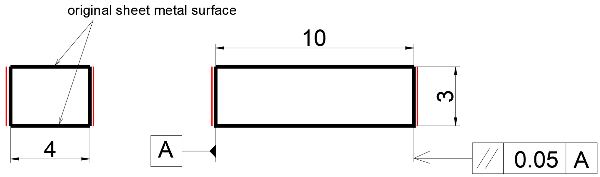
2.2. Preparation of Samples for Dilatometric Analysis
2.3. Determination of the Dilatometric Curve
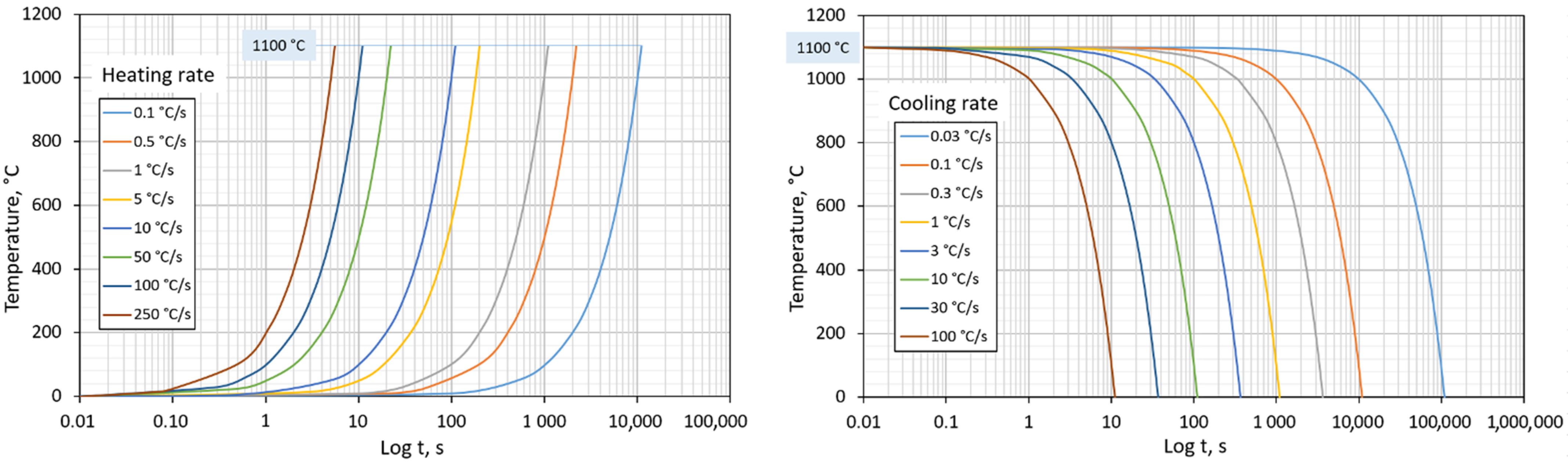
- The heating rate’s effect on shifts in the transformation temperatures, Ac1 and Ac3. For this experiment, eight variants with different heating rate values were useds from 0.1 °C/s to 250 °C/s. The cooling method was not considered. These variants are listed in Table 4 (aligning with increasing heating rate). Program control cycles are shown in Figure 3 (left).
- The cooling rate affects the resulting austenite transformation temperatures in the cooling phase, microstructure, and hardness. We used eight variants with different cooling rates from 0.03 °C/s to 100 °C/s for this experiment. The heating method was not considered. These variants are listed in Table 5 (aligning with increasing cooling rate). Program control cycles are shown in Figure 3 (right). Subsequently, a CCT diagram was created from the data analysis.
- The effect of heating and cooling rates on the resulting grain size. All variants listed in Table 3 were used for this experiment. Out of these, variants have a constant heating rate but a different cooling rate. Variants with significantly different heating rates were used but with a constant cooling rate. We assessed which parameter (heating or cooling rate) would have a greater effect on the resulting grain size.
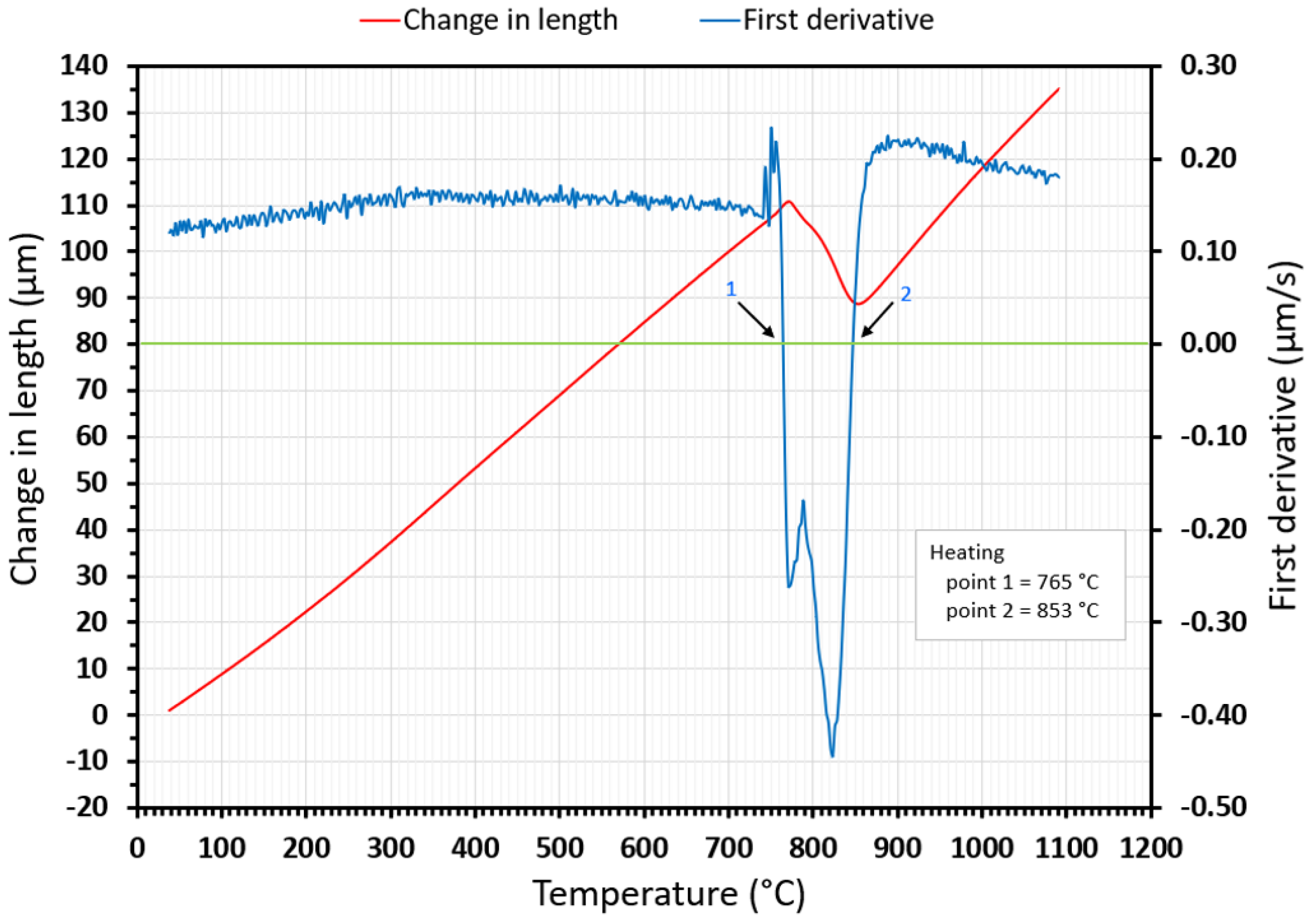
2.4. Methodology for Determining Phase Transition Temperatures from Dilatometry Curves
2.5. Microstructure Observation and Hardness Measuring
3. Results and Discussion
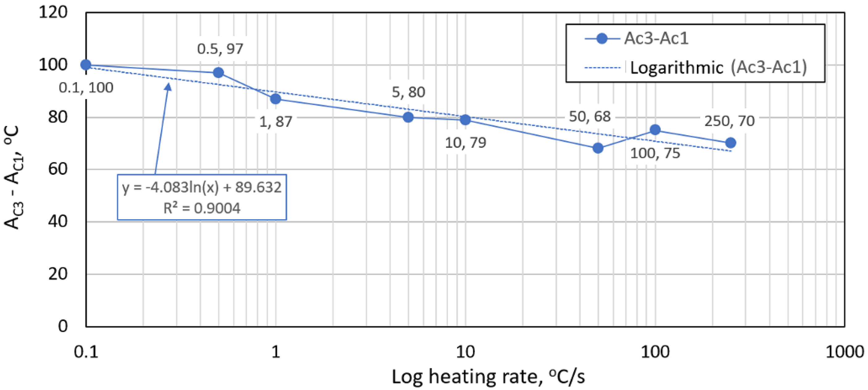
3.1. The Heating Rate’s Effect on Shifts in the Transformation Temperatures Ac1 and Ac3
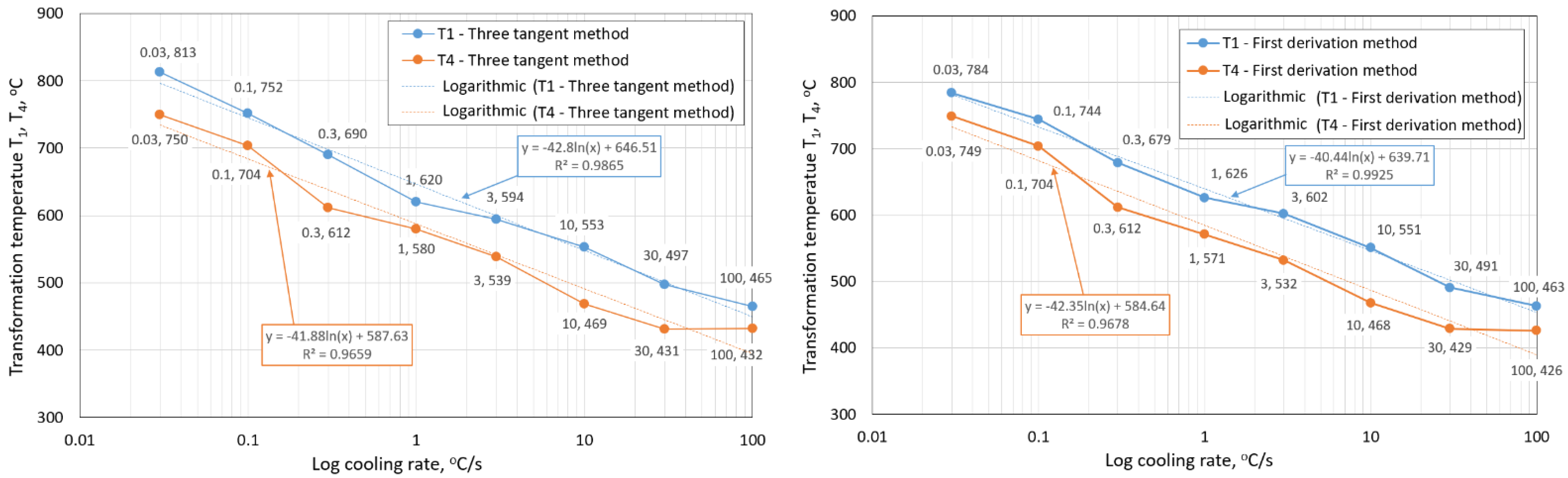
3.2. Austenite Transformation Temperatures in Cooling Phase
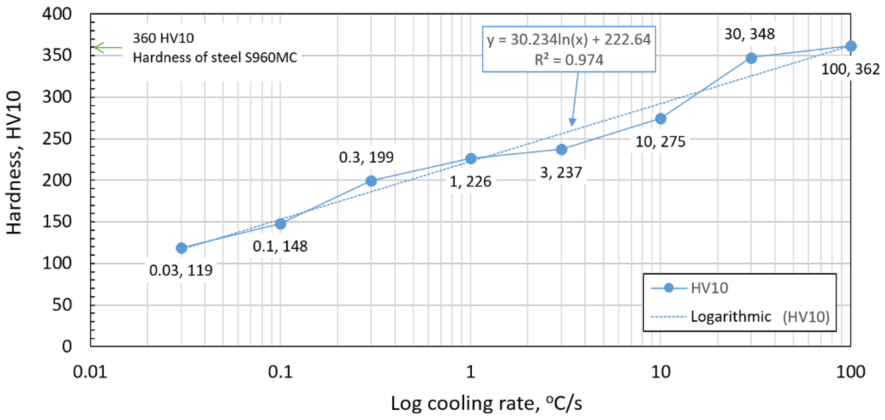
3.3. The Analysis of the Hardness after Cooling
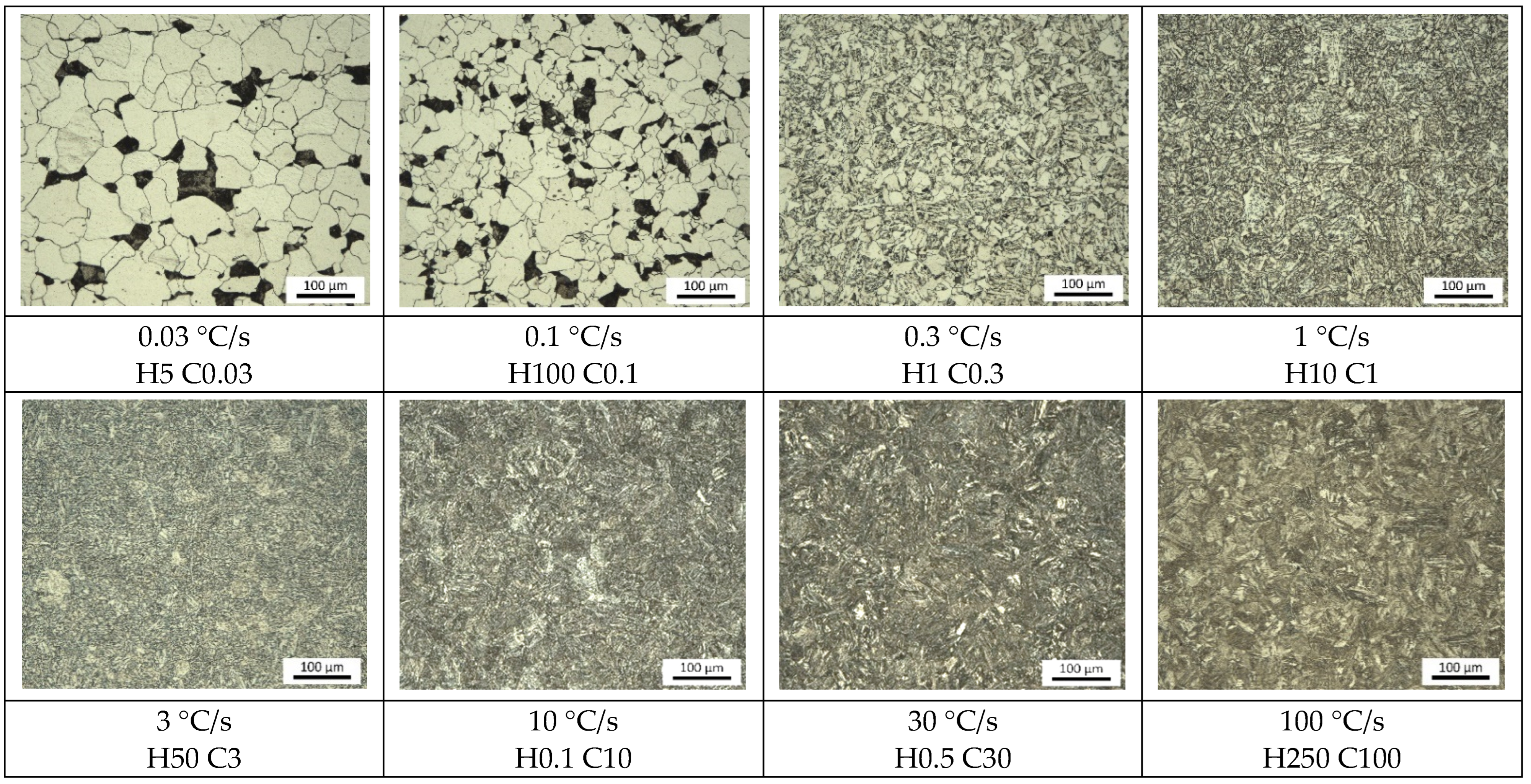
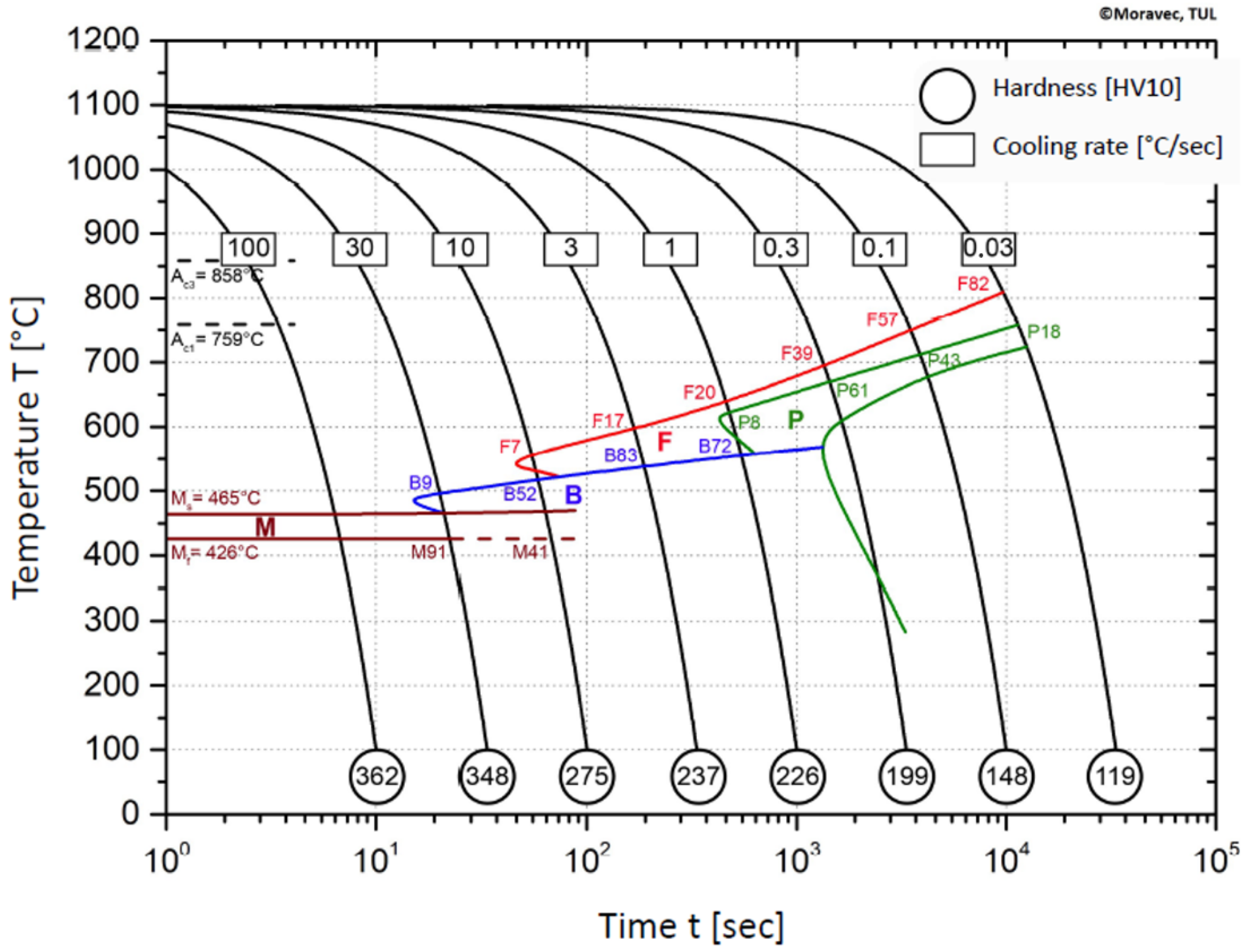
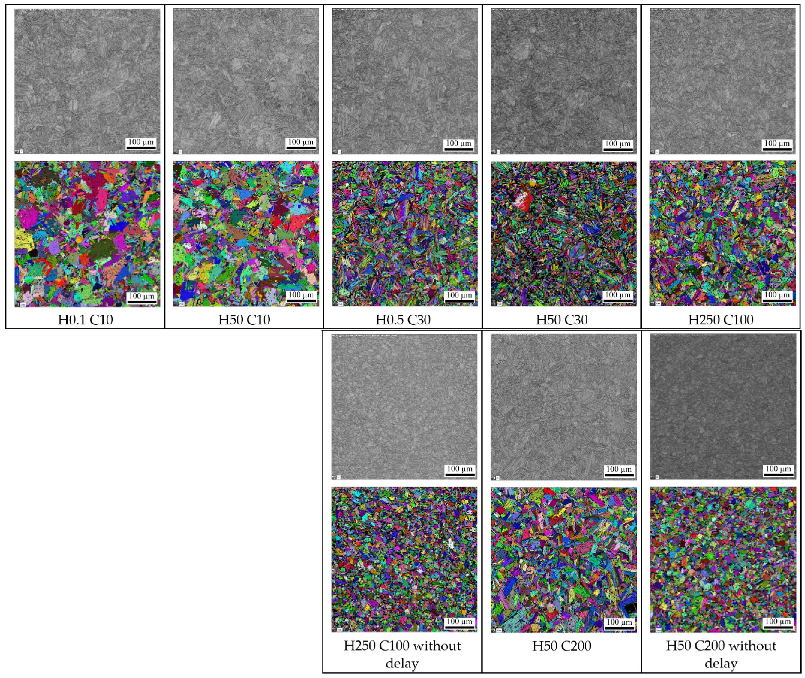
3.4. The Microstructural Analysis and Design of CCT Diagram
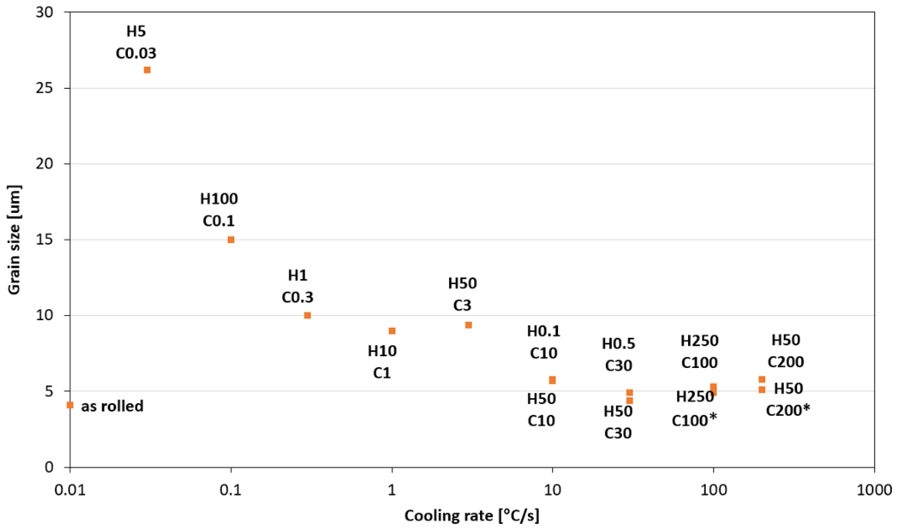
3.5. The Effect of Heating and Cooling Rates on the Resulting Grain Size
4. Conclusions
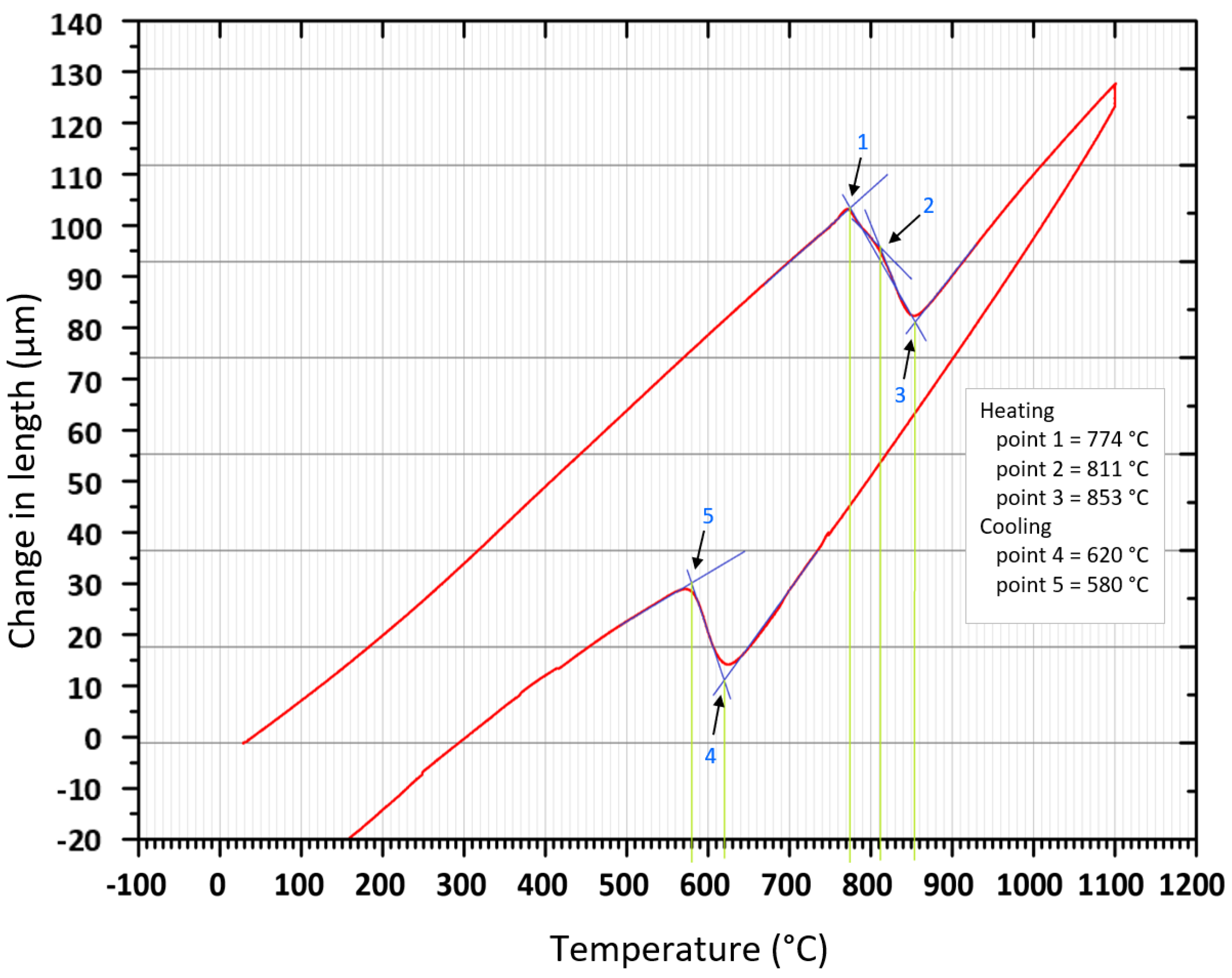
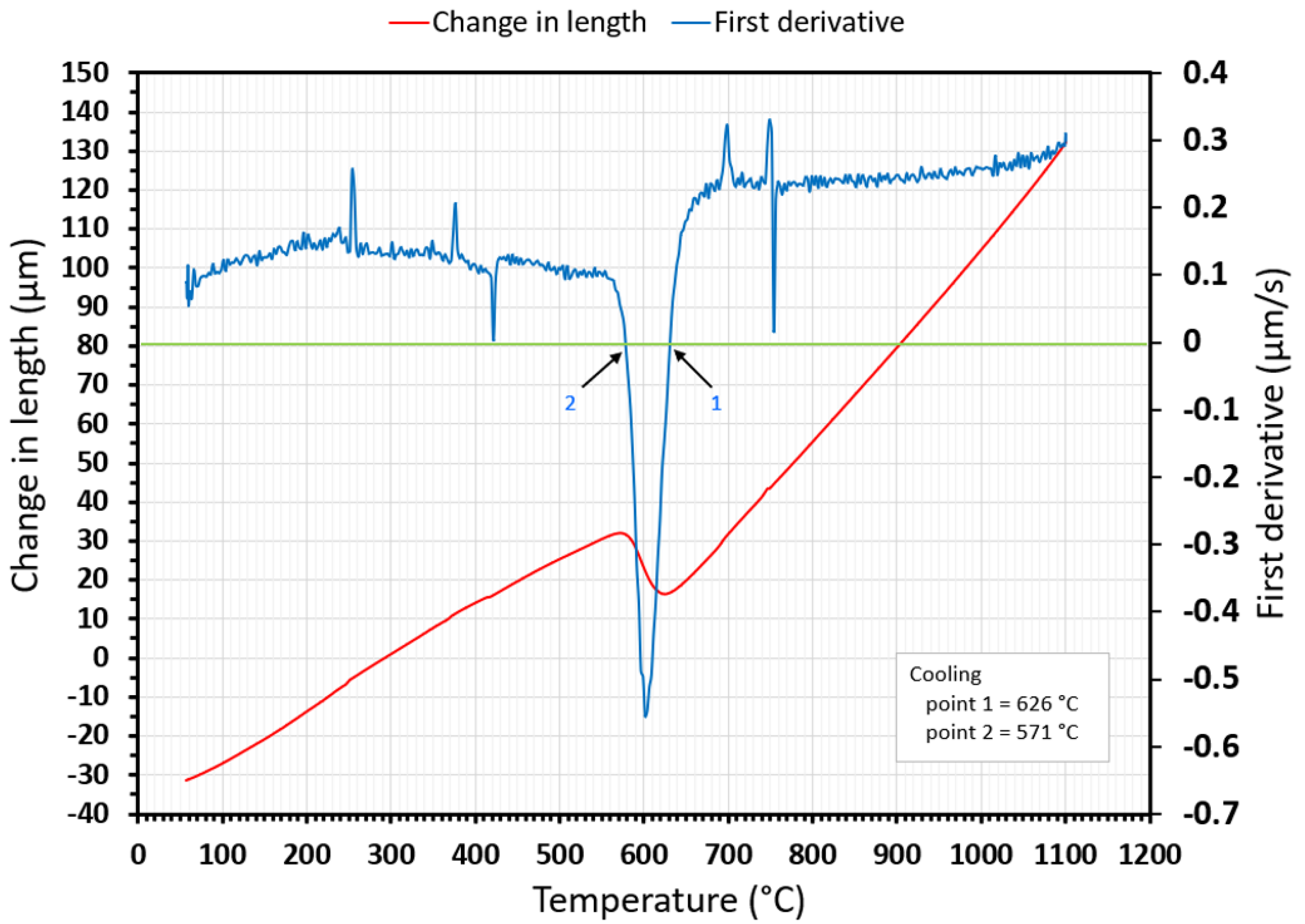
- Both methods, the three tangent method and the first derivation of the dilatometry curve method, are suitable for determining transformation temperatures. The deviation of the first derivation method from the tangent method was a maximum of 2.1% (determination of transformation temperatures in the heating phase) and a maximum of 3.7% (determination of transformation temperatures in the cooling phase).
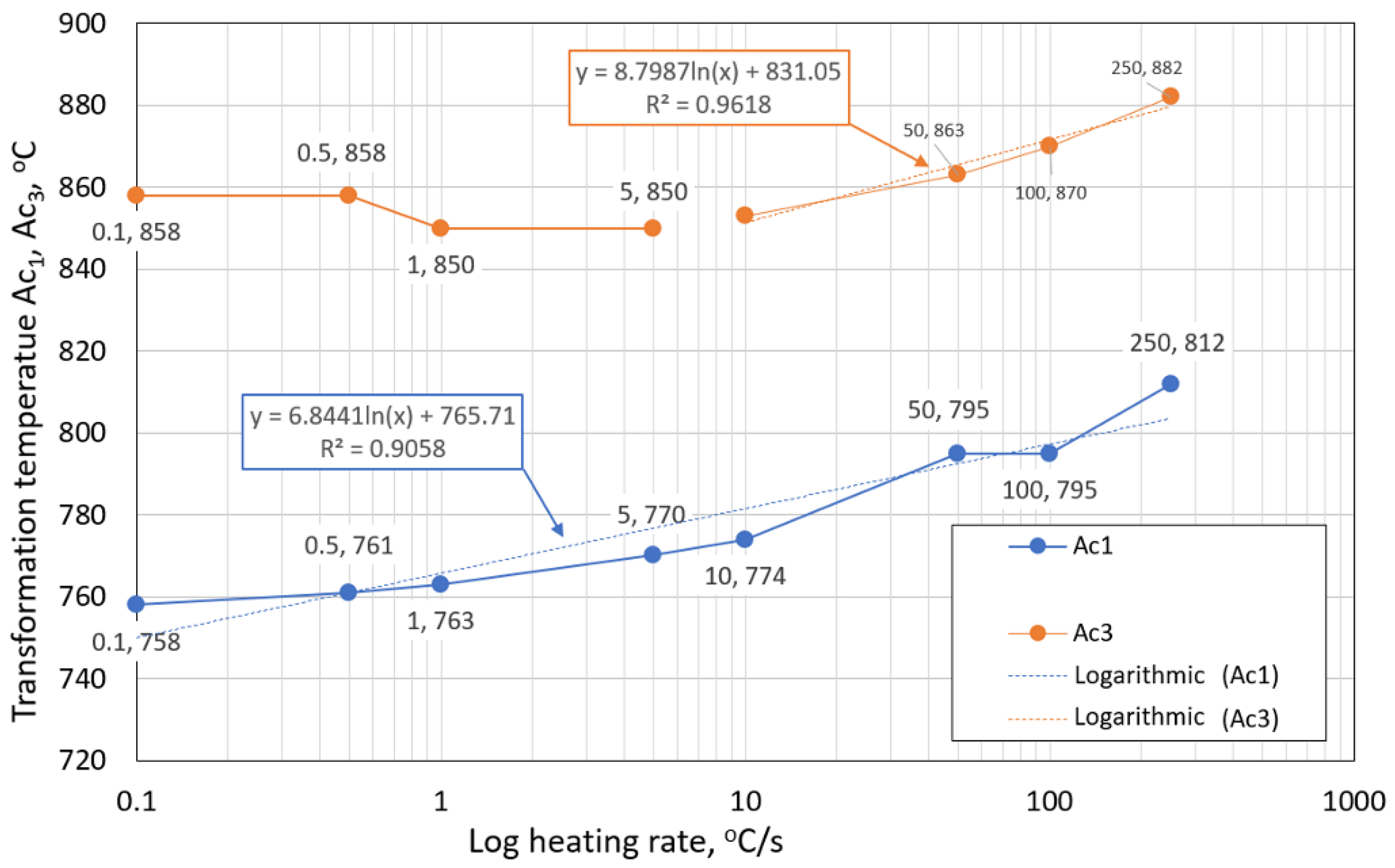
- The austenitic transformation (Ac1 temperature) increases with an increased heating rate. The dependence of these two parameters was tested by regression analysis. A linear regression model with a logarithmic function was used, which demonstrated the strong dependence of parameters (coefficient of determination was R2 = 0.9). This analysis shows that in the range of heating rates from 0.1 to 250 °C/s, the temperature Ac1 increased from 749 °C to 804 °C.
- The Ac3 temperature, when complete austenitization is achieved, was almost constant up to a heating rate of 5 °C/s (average value was 854 °C and standard deviation was 4 °C). At heating rates higher than 10 °C/s, it began to grow. From a heating rate of 10 °C/s to 250 °C/s the dependence was also described by a logarithmic function with coefficients of determination equal to R2 = 0.96. The phenomena described are important in creating the width of the heat-affected zone and welding process modeling. The welding processes with a high heating rate of the base material (laser welding and electron beam welding) will be characterized by a narrow HAZ. This eliminates the “softening effect of HAZ” that is typical for HSLA steel welding.
- The dependence of the cooling rate on the transformation temperatures T1 and T4 of austenite decomposition is significant and has the opposite trend as in the heating phase. As the cooling rate increases, the austenite decomposition temperature decreases. A linear regression model with a logarithmic function was used, which demonstrated the strong dependence of parameters (coefficient of determination was R2 = 0.98 for temperature T1 and R2 = 0.97 for temperature T4). The data are valid for the three tangent method. This analysis shows that in the range of cooling rates from 0.03 °C/s to 100 °C/s, the temperature T1 increased from 796 °C to 449 °C and temperature T4 increased from 734 °C to 394 °C.
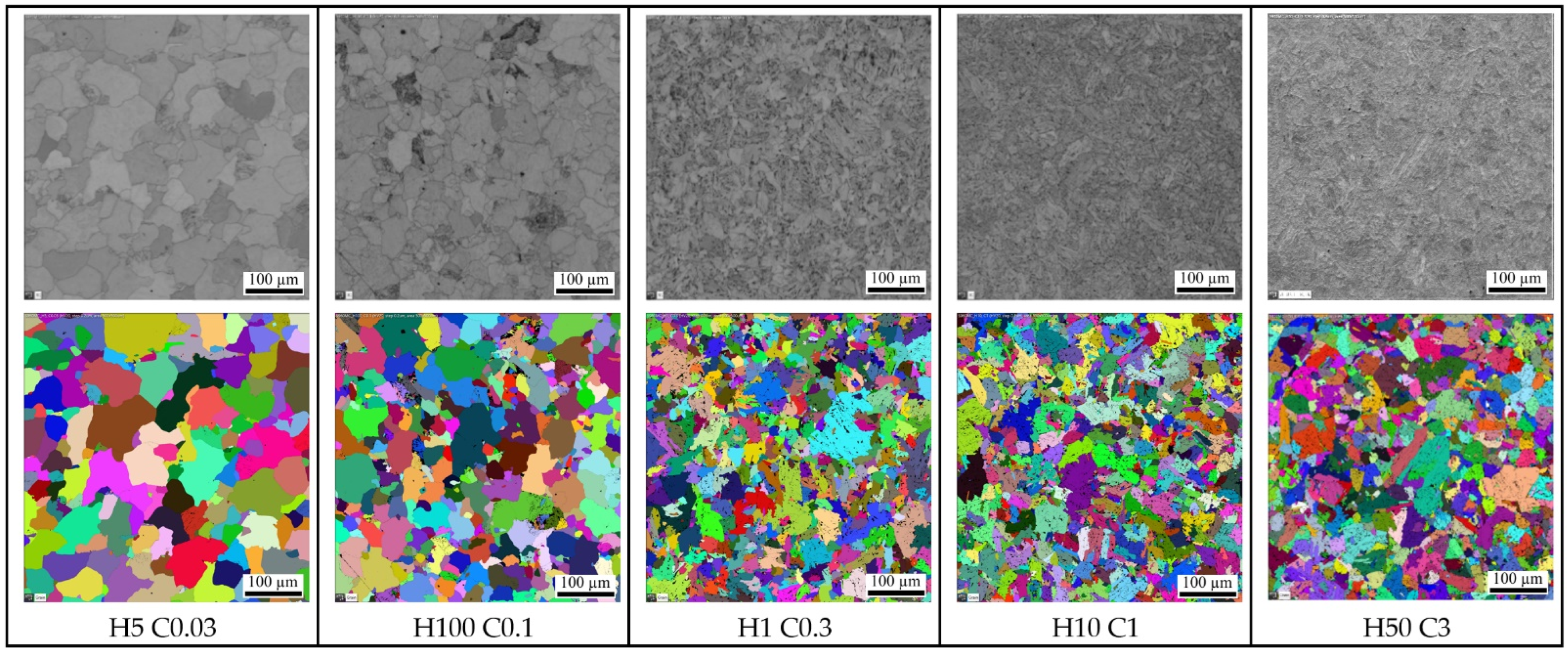
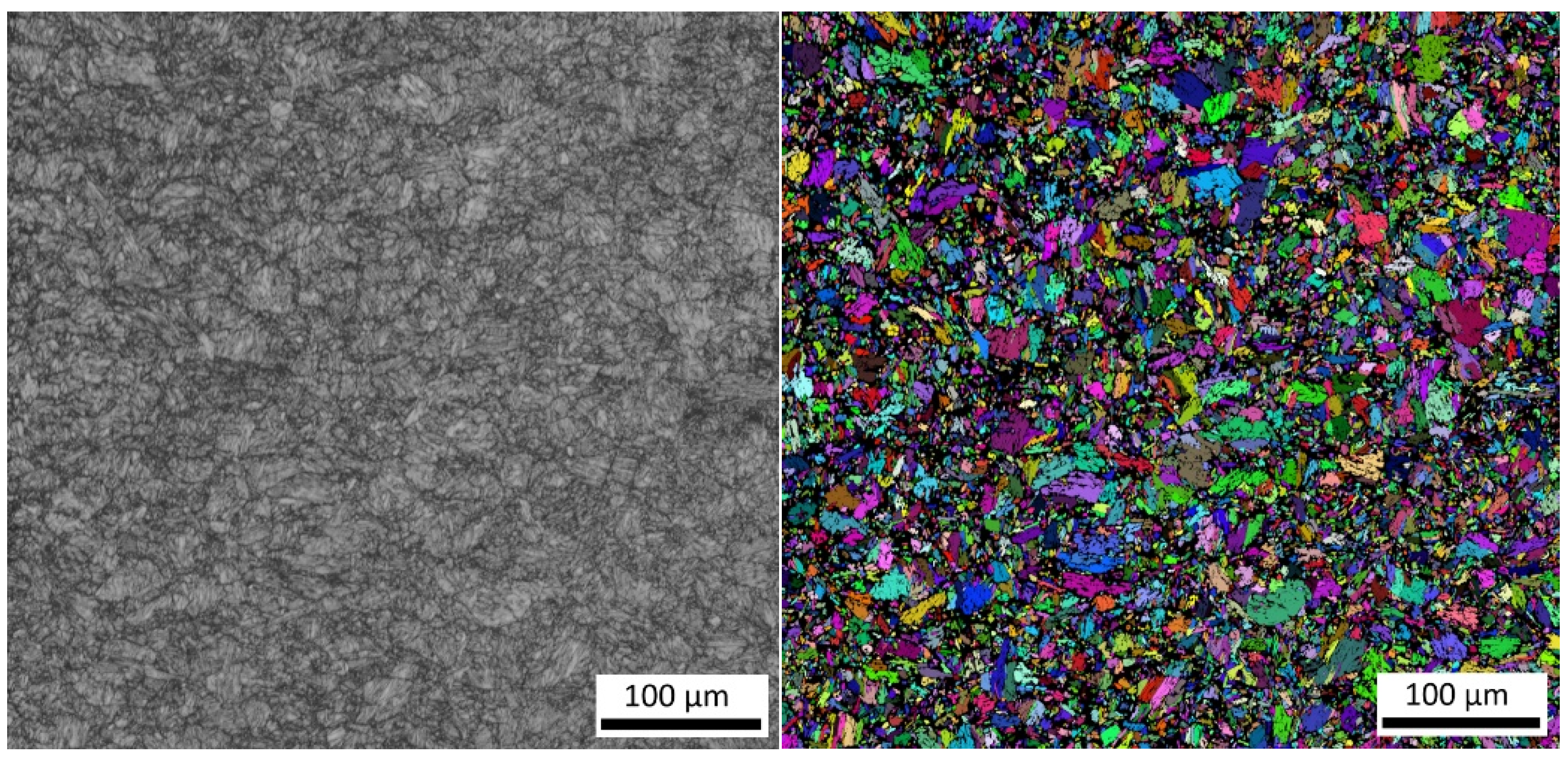
- A slow cooling rate and high transformation temperature are typical signs of diffusion transformation of austenite to ferrite or perlite. The microstructure of steel at a cooling rate of 1 °C/s and 3 °C/s comprises a mixture of ferrite and bainite (bainite predominates). Martensite appears in the microstructure only at a cooling rate of 10 °C/s. Its content increases with the increased cooling rate. At a cooling rate of 30 °C/s, its content is at the level of 91% and at a cooling rate of 100 °C/s the microstructure is fully martensitic.
- The hardness of the samples increased with the increased cooling rate due to the higher percentage of hardness phases such as bainite and martensite. The dependence of these two parameters was tested by regression analysis as well. A linear regression model with a logarithmic function was used. The coefficient of determination was R2 = 0.97, which means a strong tightness of the variables and a well-chosen regression function. This analysis shows that in the range of cooling rates from 0.03 °C/s to 100 °C/s, the hardness increased from 116 HV10 to 362 HV10. The hardness of the base material 360HV10 will be achieved according to this model at a cooling rate of 94 °C/s. This cooling rate represents a time t8/5 of 3.6 s, which can be achieved by using concentrated heat source welding methods.
- As the cooling rate increases, a trend of decreasing average grain size can be observed. However, regression analysis did not show strong parameter tightness using the full cooling rate range (from 0.03 °C/s to 100 °C/s). The coefficient of determination was R2 = 0.72 for the logarithmic regression function and R2 = 0.85 for the power regression function. Data selection and analysis, however, demonstrated these findings. We can state that the cooling rate significantly affects grain size. Variants (H50 C3, H50 C10 and H50 C30) confirmed this finding when the heating rate was constant (50 °C/s), and grain size significantly decreased from 9.4 µm to 4.4 µm with the rising cooling rate (from 3 °C/s to 30 °C/s). This represents a decrease of 53% with a cooling rate change of 27 °C/s. The effect of the heating rate is not significant on the change in grain size. The cooling rate was constant for variants H50 C10 and H0.1 C10 (10 °C/s), and the heating rates were 0.1 and 50 °C/s at the same grain size (5.7 µm and 5.8 µm). The difference in grain size in these two variants is up to 2% with a change in heating rate of approximately 50 °C/s. It was also confirmed at the tests for the cooling rate of 30 °C/s and heating rates of 0.5 and 50 °C/s. The difference in grain size for both cases was <10%.
Author Contributions
Funding
Institutional Review Board Statement
Informed Consent Statement
Data Availability Statement
Conflicts of Interest
References
- Garcia, C.I. High strength low alloyed (HSLA) steels. In Automotive steels: Design, Metallurgy, Processing and Applications, 1st ed.; Rana, R., Singh, S.B., Eds.; Woodhead Publishing: Cambridge, UK, 2016; pp. 145–167. [Google Scholar]
- Kaščák, L.; Cmorej, D.; Spišák, E.; Slota, J. Joining the High-Strength Steel Sheets Used in Car Body Production. Adv. Sci. Technol. Res. J. 2021, 15, 184–196. [Google Scholar] [CrossRef]
- Guo, W.; Li, L.; Dong, S.; Crowther, D.; Thompson, A. Comparison of microstructure and mechanical properties of ultra-narrow gap laser and gas-metal-arc welded S960 high strength steel. Opt. Lasers Eng. 2016, 91, 1–15. [Google Scholar] [CrossRef] [Green Version]
- Ghafouri, M.; Ahn, J.; Mourujärvi, J.; Björk, T.; Larkiola, J. Finite element simulation of welding distortions in ultra-high strength steel S960 MC including comprehensive thermal and solid-state phase transformation models. Eng. Struct. 2020, 219, 110804. [Google Scholar] [CrossRef]
- Tomków, J.; Landowski, M.; Fydrych, D.; Rogalski, G. Underwater wet welding of S1300 ultra-high strength steel. Mar. Struct. 2022, 81, 103120. [Google Scholar] [CrossRef]
- Górka, J.; Janicki, D.; Fidali, M.; Jamrozik, W. Thermographic Assessment of the HAZ Properties and Structure of Thermomechanically Treated Steel. Int. J. Thermophys. 2017, 38, 183. [Google Scholar] [CrossRef] [Green Version]
- Hrivňák, I. Welding and Weldability of Materials. In Zváranie a Zvariteľnosť Materiálov; Citadella: Bratislava, Slovakia, 2013. (In Slovak) [Google Scholar]
- Zhao, J.; Jiang, Z.; Kim, J.S.; Lee, C.S. Effects of tungsten on continous cooling transformation charakteristics of microalloyed steel. Mater. Des. 2013, 49, 252–258. [Google Scholar] [CrossRef] [Green Version]
- Villalobos, J.C.; Del-Pozo, A.; Campillo, B.; Mayen, J.; Serna, S. Microalloyed Steels trough History until 2018: Review of Chemical Composition, Processing and Hydrogen Service. Metals 2018, 8, 351. [Google Scholar] [CrossRef] [Green Version]
- Gu, Y.; Tian, P.; Wang, X.; Han, X.-L.; Liao, B.; Xiao, F.-R. Non-isothermal prior austenite grain growth of a high-Nb X100 pipeline steel during a simulated welding heat cycle process. Mater. Des. 2016, 89, 589–596. [Google Scholar] [CrossRef]
- Karmakar, A.; Biswas, S.; Mukherjee, S.; Chakrabarti, D.; Kumar, V. Effect of composition and thermo-mechanical processing schedule on the microstructure, precipitation and strengthening of Nb-microalloyed steel. Mater. Sci. Eng. A 2017, 690, 158–169. [Google Scholar] [CrossRef]
- Nishioka, K.; Ichikawa, K. Progres in thermomechanical control of steel plates and their commercialization. Sci. Technol. Adv. Mater. 2012, 13, 023001. [Google Scholar] [CrossRef]
- Lagneborg, R.; Hutchinson, B.; Siwecki, T.; Zajac, S. The role of vanandium in microalloyed steels. Scand. J. Metall. 1999, 28, 186–241. [Google Scholar]
- Porter, D.; Laukkanen, A.; Nevasmaa, P.; Rahka, K.; Wallin, K. Performance of TMCP steel with respect to mechanical properties after cold forming and post-forming heat treatment. Int. J. Press. Vessels Pip. 2004, 81, 867–877. [Google Scholar] [CrossRef]
- Hochhauser, F.; Ernst, W.; Rauch, R.; Vallant, R.; Enzinger, N. Influence of the Soft Zone on The Strength of Welded Modern Hsla Steels. Weld. World 2013, 56, 77–85. [Google Scholar] [CrossRef]
- Gáspár, M. Effect of Wleding Heat Input on Simulated HAZ Areas in S960QL High Strength Steel. Metals 2019, 9, 1226. [Google Scholar] [CrossRef] [Green Version]
- Pisarski, H.G.; Dolby, R.E. The Significance of Softened HAZs in High Strength Structural Steels. Weld. World 2003, 47, 32–40. [Google Scholar] [CrossRef]
- Bayock, F.N.; Kah, P.; Mvola, B.; Layus, P. Effect of Heat Input and Undermatched Filler Wire on the Microstructure and Mechanical Properties of Dissimilar S700MC/S960QC High-Strength Steels. Metals 2019, 9, 883. [Google Scholar] [CrossRef] [Green Version]
- Lahtinen, T.; Vilaça, P.; Peura, P.; Mehtonen, S. MAG Welding Tests of Modern High Strength Steels with Minimum Yield Strength of 700 MPa. Appl. Sci. 2019, 9, 1031. [Google Scholar] [CrossRef] [Green Version]
- Schneider, C.; Ernst, W.; Schnitzer, R.; Staufer, H.; Vallant, R.; Enzinger, N. Welding of S960MC with undermatching filler material. Weld. World 2018, 62, 801–809. [Google Scholar] [CrossRef] [Green Version]
- Mičian, M.; Harmania, D.; Nový, F.; Winczek, J.; Moravec, J.; Trško, L. Effect of the t8/5 cooling time on the properties of S960MC steel in the HAZ of welded joint evaluated by thermal physical simulation. Metals 2020, 10, 229. [Google Scholar] [CrossRef] [Green Version]
- Stemne, D.; Naström, T.; Thorstensson, O.; Bäckström, C. Welding Handbook, a Guide to Better Welding of HARDOX and STRENX; Höglund Design AB: Oxelosund, Sweden, 2019. [Google Scholar]
- Vimalraj, C.; Kah, P.; Layus, P.; Belinga, E.M.; Parshin, S. High-strength steel S960QC welded with rare earth nanoparticle coated filler wire. Int. J. Adv. Manuf. Technol. 2018, 102, 105–119. [Google Scholar] [CrossRef] [Green Version]
- Guo, W.; Crowther, D.; Francis, J.A.; Thompson, A.; Liu, Z.; Li, L. Microstructure and mechanical properties of laser welded S960 high strength steel. Mater. Des. 2015, 85, 534–548. [Google Scholar] [CrossRef]
- Sága, M.; Blatnická, M.; Blatnický, M.; Dižo, J.; Gerlici, J. Research of the Fatigue Life of Welded Joints of High Strength Steel S960 QL Created Using Laser and Electron Beams. Materials 2020, 13, 2539. [Google Scholar] [CrossRef] [PubMed]
- Amraei, M.; Ahola, A.; Afkhami, S.; Björk, T.; Heidarpour, A.; Zhao, X.-L. Effects of heat input on the mechanical properties of butt-welded high and ultra-high strength steels. Eng. Struct. 2019, 198, 109460. [Google Scholar] [CrossRef]
- Jambor, M.; Novy, F.; Mician, M.; Trsko, L.; Bokuvka, O.; Pastorek, F.; Harmaniak, D. Gas Metal Arc Welding of Thermo-Mechanically Controlled Processed S960MC Steel Thin Sheets with Different Welding Parameters. Commun. Sci. Lett. Univ. Zilina 2018, 20, 29–35. [Google Scholar] [CrossRef]
- Fonda, R.W.; Vandermeer, R.A.; Spanos, G. Continuous Cooling Transformation (CCT) Diagrams for Advanced Navy Welding Consumables; Naval Reasearch Laboratory: Washington, DC, USA, 1998. [Google Scholar]
- Li, X.; Shi, L.; Liu, Y.; Gan, K.; Liu, C. Achieving a desirable combination of mechanical properties in HSLA steel through step quenching. Mater. Sci. Eng. A 2020, 772, 138683. [Google Scholar] [CrossRef]
- Jiang, Z.; Zhao, J. Rolling of Advanced High Strength Steels; CRC Press: Boca Raton, FL, USA, 2017. [Google Scholar]
- Wu, X.; Lin, H.; Luo, W.; Jiang, H. Microstructure and microhardness evolution of thermal simulated HAZ of Q&P980 steel. J. Mater. Res. Technol. 2021, 15, 6067–6078. [Google Scholar] [CrossRef]
- Mandal, G.; Dey, I.; Mukherjee, S.; Ghosh, S. Phase transformation and mechanical properties of ultrahigh strength steels under continuous cooling conditions. J. Mater. Res. Technol. 2022, 19, 628–642. [Google Scholar] [CrossRef]
- Geng, X.; Wang, H.; Xue, W.; Xiang, S.; Huang, H.; Meng, L.; Ma, G. Modeling of CCT diagrams for tool steels using different machine learning techniques. Comput. Mater. Sci. 2020, 171, 109235. [Google Scholar] [CrossRef]
- SSAB. Available online: https://www.ssab.com/en/products/brands/strenx/products/strenx-960-mc (accessed on 8 November 2021).
- Mola, J. Dilatometry Analysis of Cementite Precipitation in Medium Mn High Carbon Steels. In Proceedings of the ICAS & HMnS, Chengdu, China, 16–18 November 2016. [Google Scholar]
- Bräutigam-Matus, K.; Altamirano, G.; Salinas, A.; Flores, A.; Goodwin, F. Experimental Determination of Continuous Cooling Transformation (CCT) Diagrams for Dual-Phase Steels from the Intercritical Temperature Range. Metals 2018, 8, 674. [Google Scholar] [CrossRef] [Green Version]
- Standard STN EN 10149-2; Hot Rolled Flat Products Made of High Yield Strength Steels for Cold Forming—Part 2: Technical Delivery Conditions for Thermomechanically Rolled Steels. Slovak Office of Standards, Metrology and Testing: Bratislava, Slovakia, 2014.
- Standard STN EN ISO 6892-1; Metallic Materials. Tensile Testing. Part 1: Method of Test at Room Temperature. Slovak Office of Standards, Metrology and Testing: Bratislava, Slovakia, 2022.
- TA Instruments. Available online: https://www.tainstruments.com/dil-805l-quenching-dilatomers/ (accessed on 20 November 2021).
- Pawlowski, B.; Bala, P.; Dziurka, R. Improrer interpretation of dilatometric data for cooling transformation in steels. Arch. Metall. Mater. 2014, 59, 1159–1161. [Google Scholar] [CrossRef] [Green Version]
- Grajcar, A.; Zalecki, W.; Skrzypczyk, P.; Kilarski, A.; Kowalski, A.; Kolodziej, S. Dilatometric study of phase transformations in advanced high-stength bainitic steel. J. Anal. Calorim. 2014, 118, 739–748. [Google Scholar] [CrossRef] [Green Version]
- Moravec, J.; Dikovits, M.; Novakova, I.; Caliskanoglu, O. Comparison of Dilatometry Results Obtained by Two Different Devices when Generating CCT and In Situ Diagrams. Key Eng. Mater. 2016, 669, 477–484. [Google Scholar] [CrossRef]
- Falkenreck, T.; Kromm, A.; Böllinghaus, T. Investigation of physically simulated weld HAZ and CCT diagram of HSLA armour steel. Weld. World 2017, 62, 47–54. [Google Scholar] [CrossRef]
- Kawulok, R.; Schindler, I.; Kawulok, P.; Rusz, S.; Opěla, P.; Solowski, Z.; Čmiel, M. Effect of Deformation on the Continuous Cooling Transformation (CCT) Diagram of Steel CrB4. Metalurgija 2015, 54, 473–476. [Google Scholar]
- Contreras, A.; López, A.; Gutiérrez, E.; Fernández, B.; Salinas, A.; Deaquino, R.; Bedolla, A.; Saldaña, R.; Reyes, I.; Aguilar, J.; et al. An approach for the design of multiphase advanced high-strength steels based on the behavior of CCT diagrams simulated from the intercritical temperature range. Mater. Sci. Eng. A 2019, 772, 138708. [Google Scholar] [CrossRef]
- Skočovský, P.; Bokůvka, O.; Konečná, R.; Tillová, E. Náuka o Materiáli; EDIS: Žilina, Slovakia, 2014.
- Schindler, I.; Kawulok, R.; Opěla, P.; Kawulok, P.; Rusz, S.; Sojka, J.; Sauer, M.; Navrátil, H.; Pindor, L. Effects of Austenitization Temperature and Pre-Deformation on CCT Diagrams of 23MnNiCrMo5-3 Steel. Materials 2020, 13, 5116. [Google Scholar] [CrossRef] [PubMed]
- Kamyabi-Gol, A.; Herath, D.; Mendez, P.F. A comparison of common and new methods to determine martensite start temperature using a dilatometer. Can. Met. Q. 2017, 56, 85–93. [Google Scholar] [CrossRef]


| According | Chemical Composition wt.%—Strenx 960MC | ||||||||||
|---|---|---|---|---|---|---|---|---|---|---|---|
| C | Si | Mn | P | S | Al | Nb | V | Ti | Mo | B | |
| EN 10149-2 * | 0.200 | 0.60 | 2.200 | 0.025 | 0.010 | 0.015 | 0.090 | 0.200 | 0.250 | 1.000 | 0.005 |
| Material certificate ** | 0.085 | 0.180 | 1.060 | 0.010 | 0.003 | 0.036 | 0.002 | 0.007 | 0.026 | 0.109 | 0.001 |
| Experimental measurement average value/standard deviation | 0.055/ 0.0024 | 0.168/ 0.0045 | 1.203/ 0.0047 | <0.010 | <0.010 | 0.037/ 0.00023 | <0.005 | 0.005/ 0.00025 | 0.023/ 0.00017 | 0.086/ 0.00012 | - |
| Cu | Cr | Ni | N | CEV | CET | ||||||
| EN 10149-2 * | - | - | - | - | - | - | |||||
| Material certificate ** | 0.010 | 1.080 | 0.070 | 0.005 | 0.506 | 0.258 | |||||
| Experimental measurement average value/standard deviation | <0.005 | 1.056/ 0.0081 | 0.046/ 0.0017 | - | 0.489 | 0.238 | |||||
| According | Angle of Rolling Direction | Mechanical Properties S960MC, Thickness 3 mm | ||||||
|---|---|---|---|---|---|---|---|---|
| Rp0.2 [MPa] | Rm [MPa] | Rp0.2/Rm | A [%] | |||||
| EN 10149-2 | - | min. 960 | 980–1250 | - | min. 7 | |||
| Average Rp0.2 [Mpa]/Standard deviation [Mpa] | Average Rm [Mpa]/Standard deviation [Mpa] | Average Rp0.2/Average Rm | Average A [%]/Standard deviation [%] | Coefficient of area anisotropy P * [%] | ||||
| PRm | PRp0.2 | PA | ||||||
| Experimental measurement | 0° | 1007/15.6 | 1092/7.3 | 0.92 | 7.9/0.28 | - | - | - |
| 45° | 1018/5.1 | 1106/7.4 | 0.92 | 6.7/0.16 | 1.2 | 1.1 | −14.4 | |
| 90° | 1044/7.3 | 1124/4.6 | 0.93 | 6.5/0.05 | 2.9 | 3.6 | −17.0 | |
| Variant Designation | H5 C0.03 | H100 C0.1 | H1 C0.3 | H10 C1 | H50 C3 | H0.1 C10 | H50 C10 |
| Heating rate °C/s | 5 | 100 | 1 | 10 | 50 | 0.1 | 50 |
| Cooling rate °C/s | 0.03 | 0.1 | 0.3 | 1 | 3 | 10 | 10 |
| Variant Designation | H0.5 C30 | H50 C30 | H250 C100 | H250 C100 * | H50 C200 | H50 C200 * | |
| Heating rate °C/s | 0.5 | 50 | 250 | 250 * | 50 | 50 * | |
| Cooling rate °C/s | 30 | 30 | 100 | 100 * | 200 | 200 * |
| Heating Rate °C/s | 0.1 | 0.5 | 1 | 5 | 10 | 50 | 100 | 250 |
|---|---|---|---|---|---|---|---|---|
| Cooling rate °C/s | 10 | 30 | 0.3 | 0.03 | 1 | 3 | 0.1 | 100 |
| Variant designation | H0.1 C10 | H0.5 C30 | H1 C0.3 | H5 C0.03 | H10 C1 | H50 C3 | H100 C0.1 | H250 C100 |
| Cooling Rate °C/s | 0.03 | 0.1 | 0.3 | 1 | 3 | 10 | 30 | 100 |
|---|---|---|---|---|---|---|---|---|
| Heating rate °C/s | 5 | 100 | 1 | 10 | 50 | 0.1 | 0.5 | 250 |
| Variant | H5C 0.03 | H100 C0.1 | H1 C0.3 | H10 C1 | H50 C3 | H0.1 C10 | H0.5 C30 | H250 C100 |
| Heating Rate [°C/s] | 0.1 | 0.5 | 1 | 5 | 10 | 50 | 100 | 250 | |
|---|---|---|---|---|---|---|---|---|---|
| Variant Designation | H0.1 C10 | H0.5 C30 | H1 C0.3 | H5 C0.03 | H10 C1 | H50 C3 | H100 C0.1 | H250 C100 | |
| Three tangent method | Ac1 [°C] | 758 | 761 | 763 | 770 | 774 | 795 | 795 | 812 |
| Ac3 [°C] | 858 | 858 | 850 | 850 | 853 | 863 | 870 | 882 | |
| First derivation method | Ac1 [°C] | 753 | 758 | 763 | 770 | 788 | 806 | 812 | 832 |
| Ac3 [°C] | 855 | 850 | 850 | 850 | 870 | 880 | 886 | 898 | |
| Difference between used methods | diff. Ac1 [%] | 0.66 | 0.40 | 0.00 | 0.00 | 1.78 | 1.36 | 2.09 | 2.40 |
| diff. Ac3 [%] | 0.35 | 0.94 | 0.00 | 0.00 | 1.95 | 1.93 | 1.81 | 1.78 | |
| Cooling Rate [°C/s] | 0.03 | 0.1 | 0.3 | 1 | 3 | 10 | 30 | 100 | |
|---|---|---|---|---|---|---|---|---|---|
| Variant Designation | H5C 0.03 | H100 C0.1 | H1 C0.3 | H10 C1 | H50 C3 | H0.1 C10 | H0.5 C30 | H250 C100 | |
| Three tangent method | T1 [°C] | 813 | 752 | 690 | 620 | 594 | 553 | 497 | 465 |
| T2 [°C] | - | 744 | - | - | - | 534 | 465 | 456 | |
| T3 [°C] | - | - | - | - | - | 514 | 469 | 442 | |
| T4 [°C] | 750 | 704 | 612 | 580 | 539 | 469 | 431 | 432 | |
| First derivation method | T1 [°C] | 784 | 744 | 679 | 626 | 602 | 551 | 491 | 463 |
| T4 [°C] | 749 | 704 | 612 | 571 | 532 | 468 | 429 | 426 | |
| Difference between used methods | diff. T1 [%] | 3.70 | 1.08 | 1.62 | 0.96 | 1.33 | 0.36 | 1.22 | 0.43 |
| diff. T4 [%] | 0.13 | 0.00 | 0.00 | 1.58 | 1.32 | 0.21 | 0.47 | 1.41 | |
| Cooling Rate [°C/s] | Variant | Hardness HV10 | Average Hardness HV10/Standard Deviation HV10 | |||||
|---|---|---|---|---|---|---|---|---|
| 0.03 | H5C 0.03 | 118 | 116 | 122 | 117 | 119 | 123 | 119/2.54 |
| 0.1 | H100 C0.1 | 152 | 145 | 157 | 144 | 148 | 143 | 148/4.94 |
| 0.3 | H1 C0.3 | 196 | 201 | 203 | 197 | 200 | 199 | 199/2.36 |
| 1 | H10 C1 | 223 | 231 | 227 | 227 | 227 | 223 | 226/2.75 |
| 3 | H50 C3 | 236 | 238 | 240 | 232 | 237 | 239 | 237/2.58 |
| 10 | H0.1 C10 | 276 | 268 | 279 | 281 | 273 | 271 | 275/4.50 |
| 30 | H0.5 C30 | 349 | 344 | 352 | 352 | 346 | 342 | 348/3.81 |
| 100 | H250 C100 | 357 | 365 | 356 | 372 | 361 | 360 | 362/5.40 |
| Base material | 362 | 363 | 357 | 362 | 360 | 358 | 360/2.21 | |
| Variant Designation | Cooling Rate [°C/s] | Grain Size ECD ** [µm] Area 500 × 500 µm, Step 0.2 µm, Average Value/Standard Deviation |
|---|---|---|
| H5 C0.03 | 0.03 | 26.2/15.94 |
| H100 C0.1 | 0.1 | 15.0/8.87 |
| H1 C0.3 | 0.3 | 10.0/7.89 |
| H10 C1 | 1 | 9.0/6.98 |
| H50 C3 | 3 | 9.4/6.01 |
| H50 C10 | 10 | 5.7/4.22 |
| H0.1 C10 | 10 | 5.8/4.71 |
| H50 C30 | 30 | 4.4/2.71 |
| H0.5 C30 | 30 | 4.9/3.17 |
| H250 C100 | 100 | 5.3/3.76 |
| H250 C100 * | 100 * | 4.9/2.89 |
| H50 C200 | 200 | 5.8/4.64 |
| H50 C200 * | 200 * | 5.1/3.19 |
| As rolled | - | 4.1/2.34 |
Publisher’s Note: MDPI stays neutral with regard to jurisdictional claims in published maps and institutional affiliations. |
© 2022 by the authors. Licensee MDPI, Basel, Switzerland. This article is an open access article distributed under the terms and conditions of the Creative Commons Attribution (CC BY) license (https://creativecommons.org/licenses/by/4.0/).
Share and Cite
Moravec, J.; Mičian, M.; Málek, M.; Švec, M. Determination of CCT Diagram by Dilatometry Analysis of High-Strength Low-Alloy S960MC Steel. Materials 2022, 15, 4637. https://doi.org/10.3390/ma15134637
Moravec J, Mičian M, Málek M, Švec M. Determination of CCT Diagram by Dilatometry Analysis of High-Strength Low-Alloy S960MC Steel. Materials. 2022; 15(13):4637. https://doi.org/10.3390/ma15134637
Chicago/Turabian StyleMoravec, Jaromír, Miloš Mičian, Miloslav Málek, and Martin Švec. 2022. "Determination of CCT Diagram by Dilatometry Analysis of High-Strength Low-Alloy S960MC Steel" Materials 15, no. 13: 4637. https://doi.org/10.3390/ma15134637
APA StyleMoravec, J., Mičian, M., Málek, M., & Švec, M. (2022). Determination of CCT Diagram by Dilatometry Analysis of High-Strength Low-Alloy S960MC Steel. Materials, 15(13), 4637. https://doi.org/10.3390/ma15134637