
A Multiphysics Model for Predicting Microstructure Changes and Microhardness of Machined AerMet100 Steel

Abstract
:1. Introduction
2. Multiphysics Modeling of Machining
2.1. Analytical Models for White Layer and Microhardness
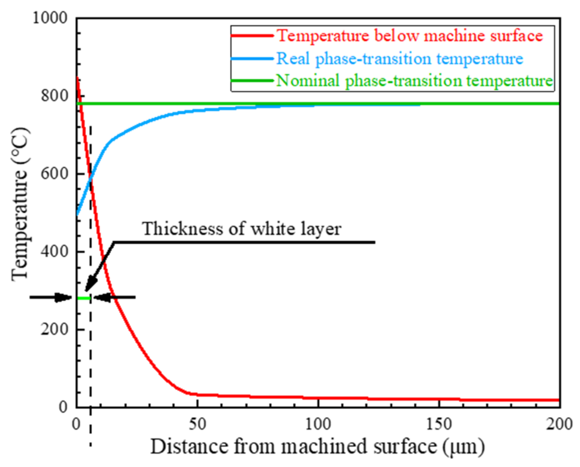
2.1.1. Model of White-Layer Generation
2.1.2. Model of Microhardness Change
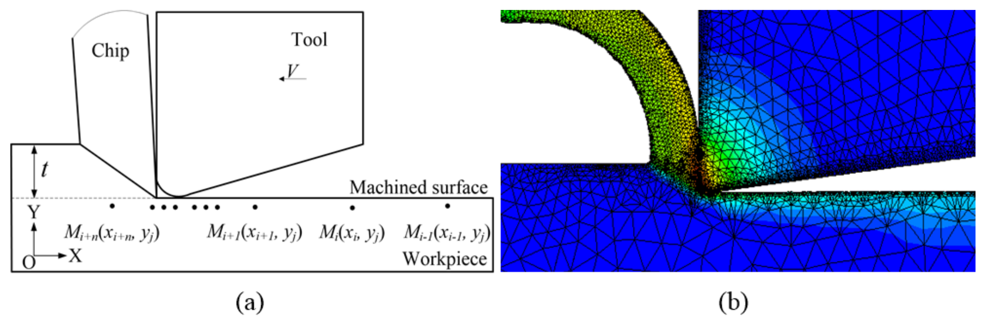
2.2. Finite-Element Model for Orthogonal Cutting
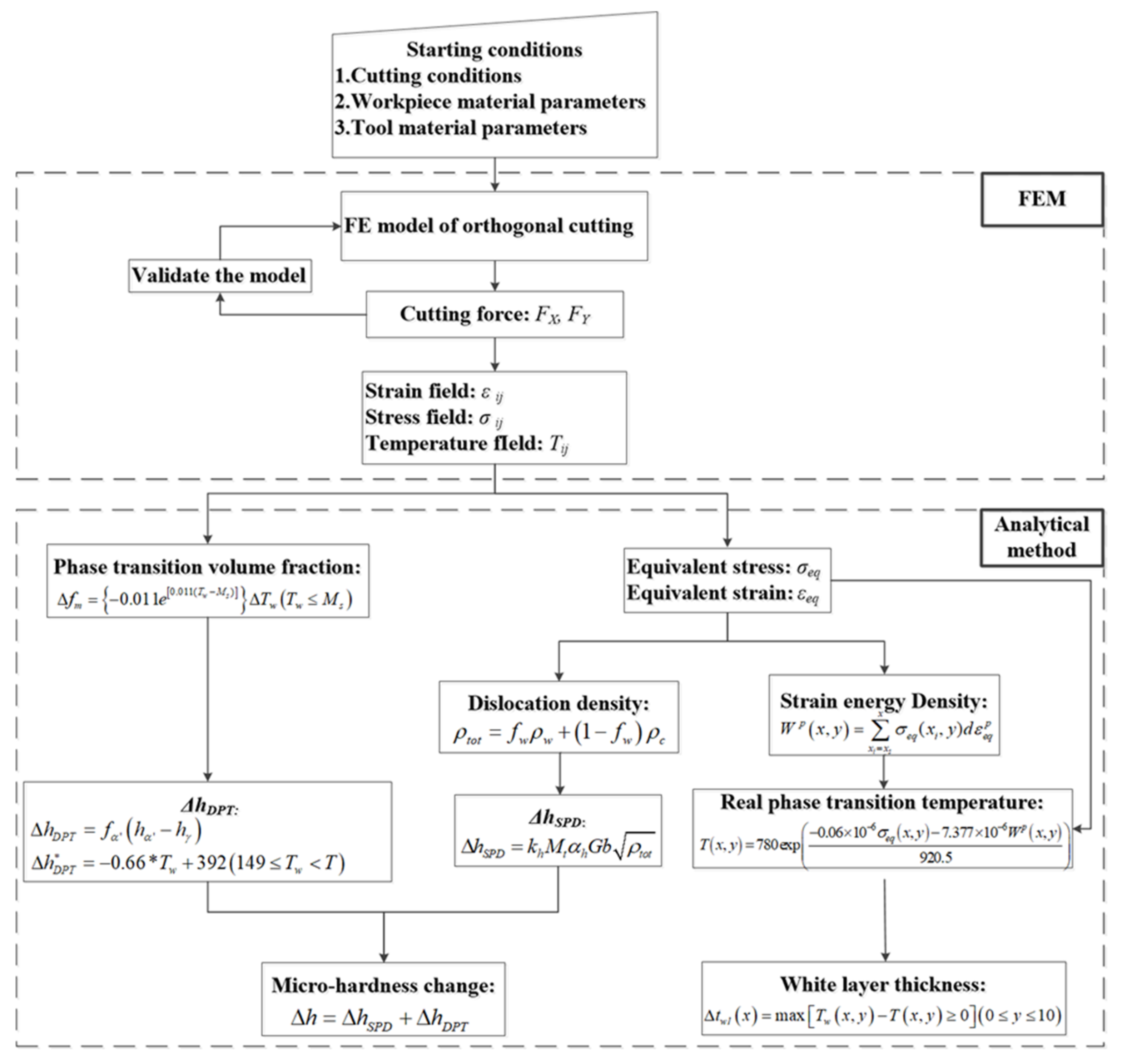
2.3. Calculation Procedure
3. Materials and Methods
3.1. Material and Machining Process
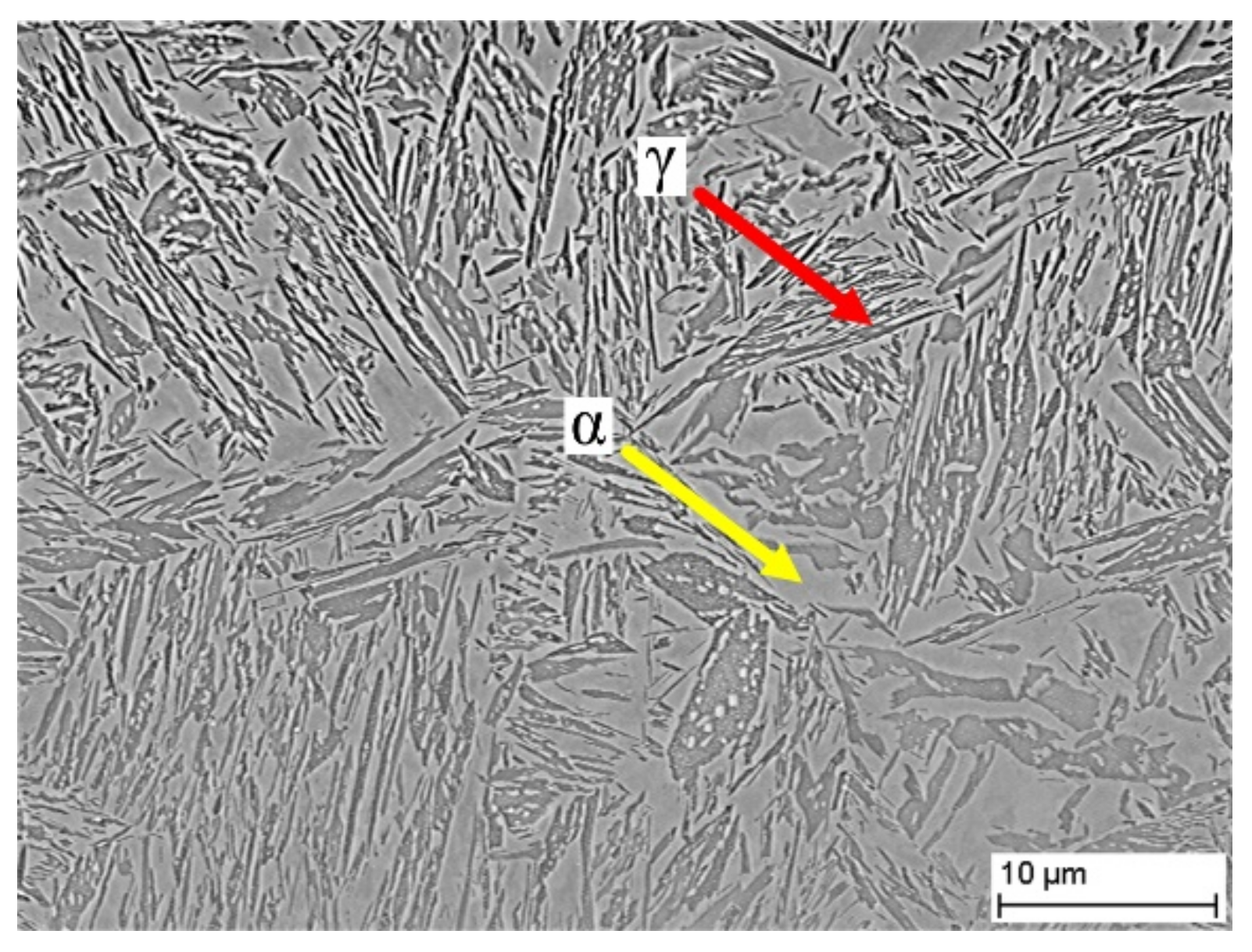
3.2. Microstructure Examination
3.3. Microhardness Measurement
3.4. XRD Measurement
4. Results
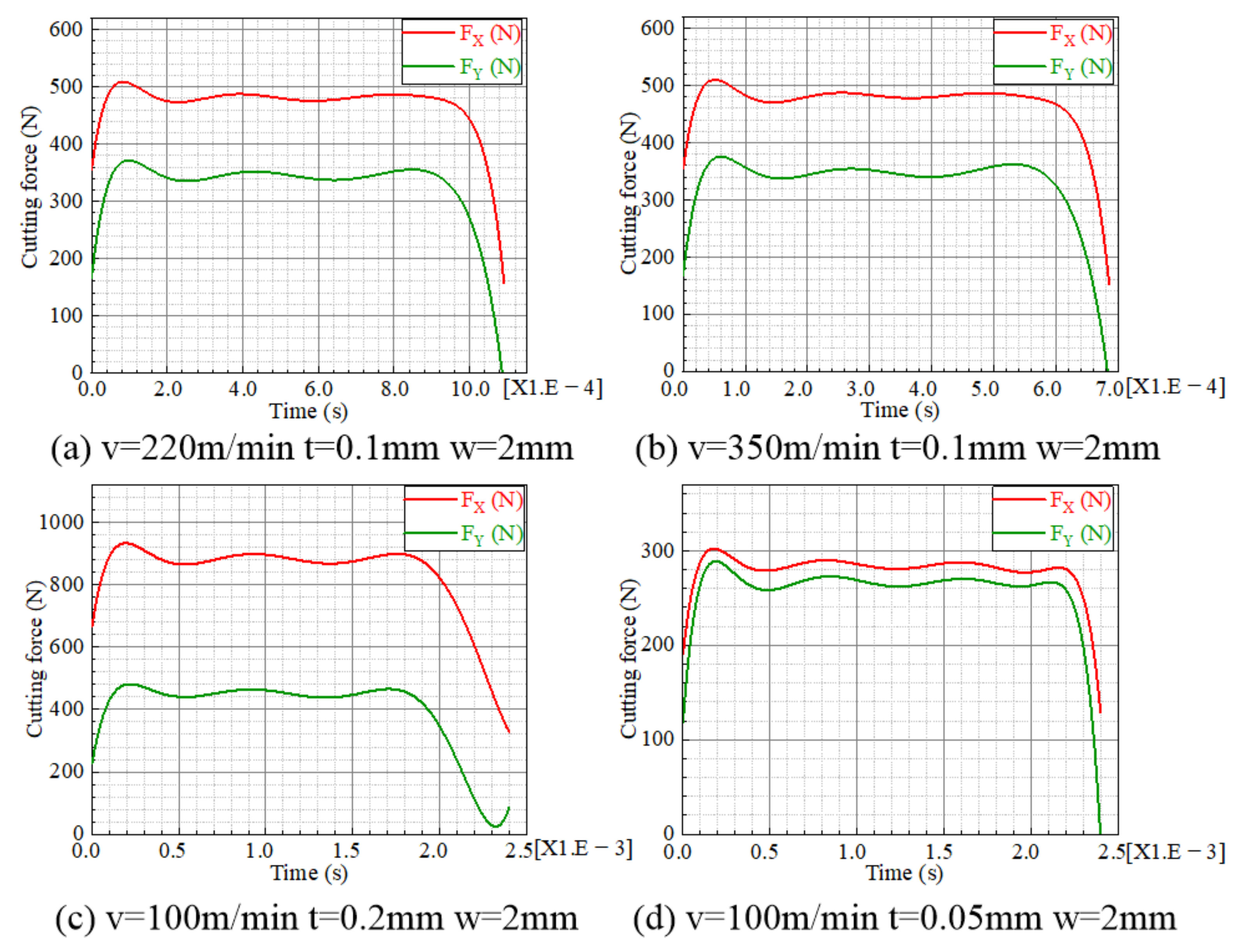
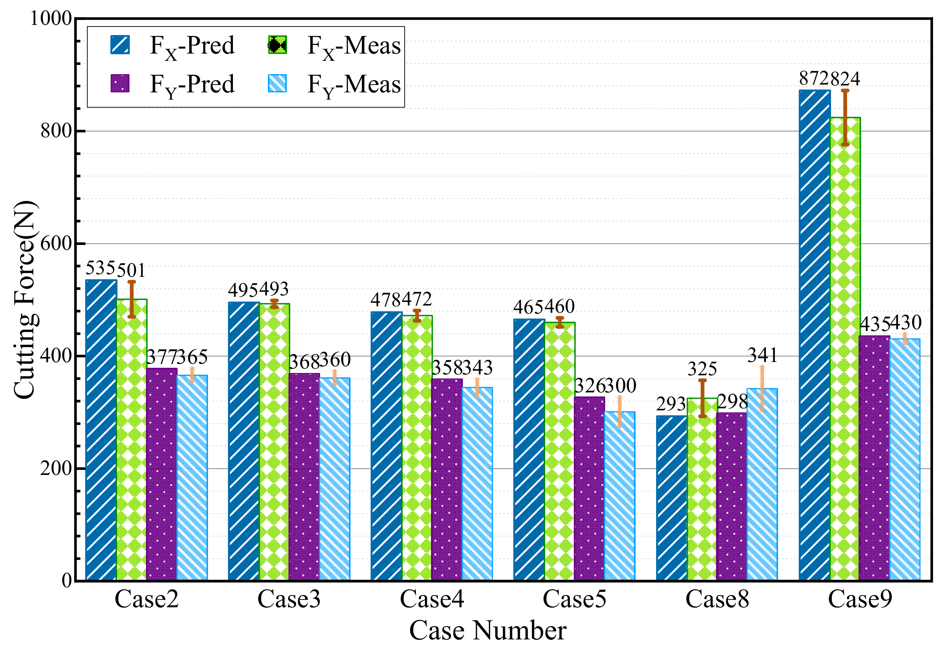
4.1. Cutting Force
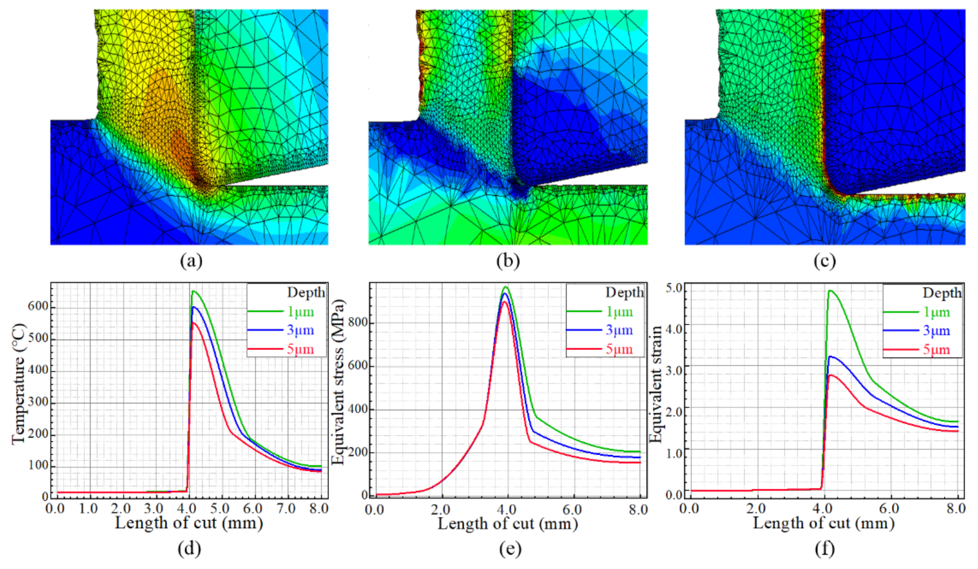
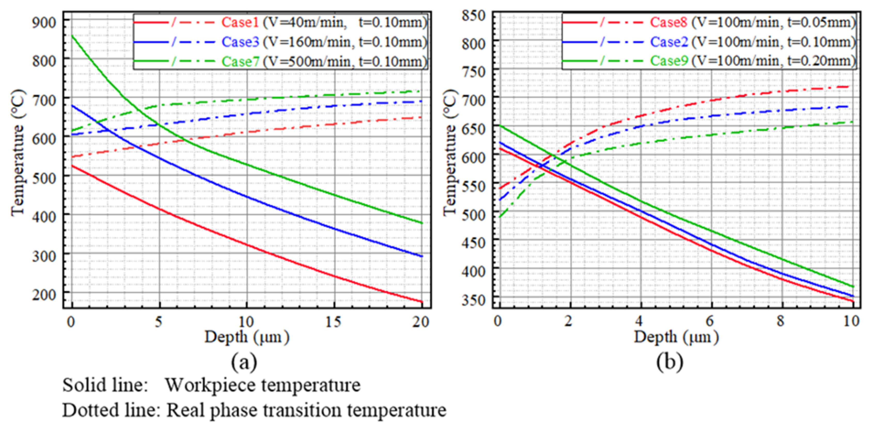
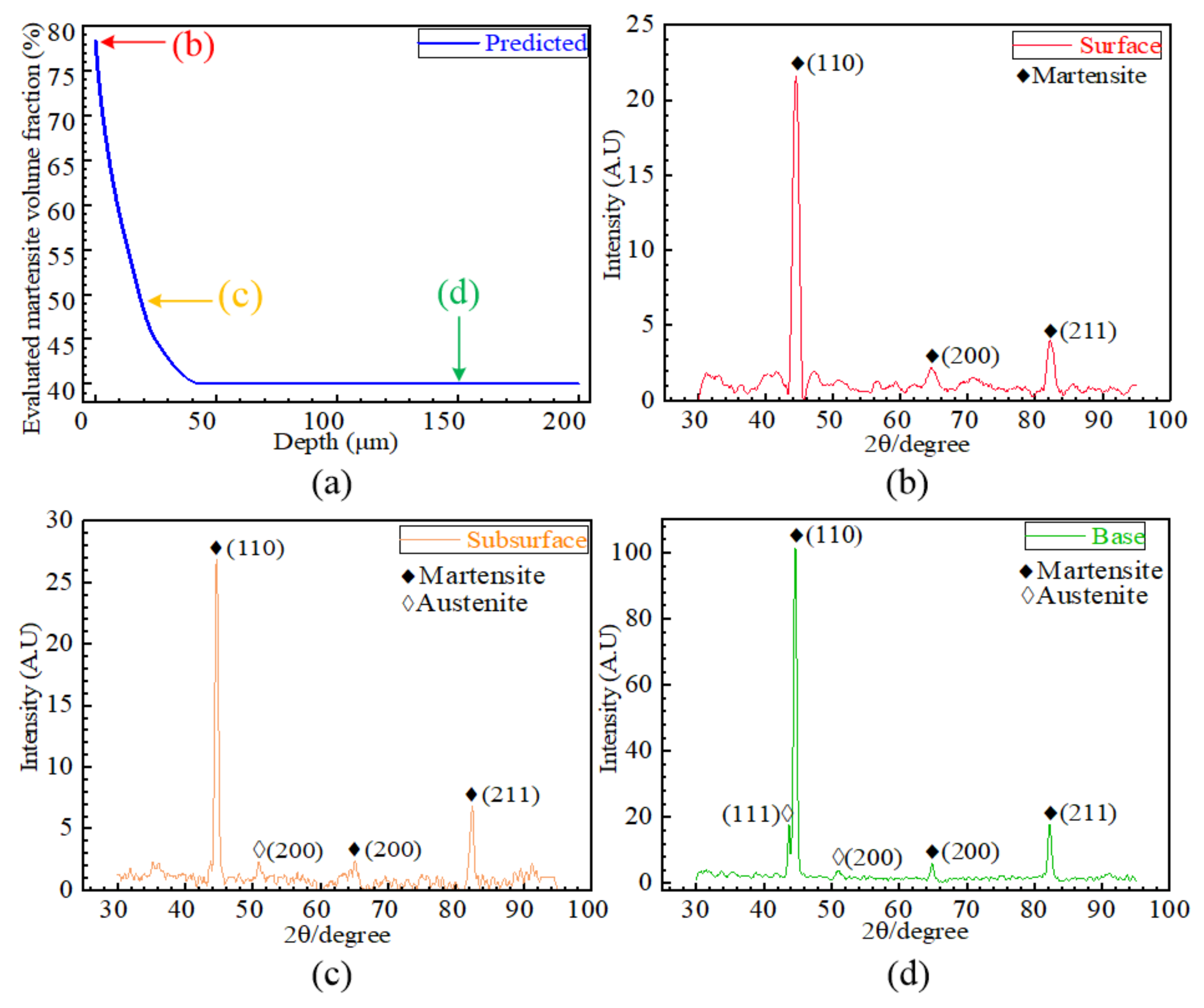
4.2. Phase Transformation
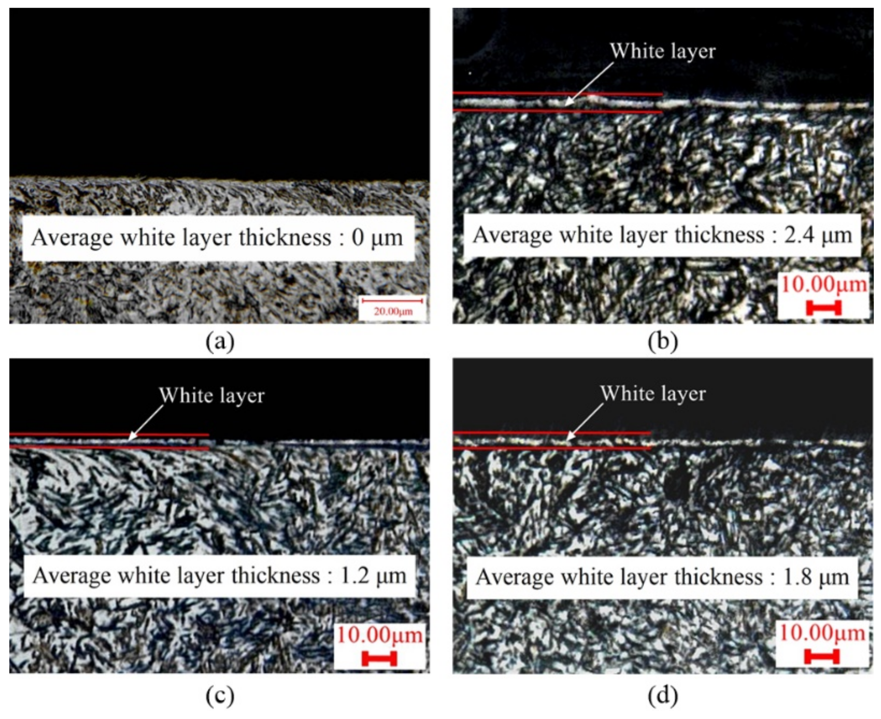
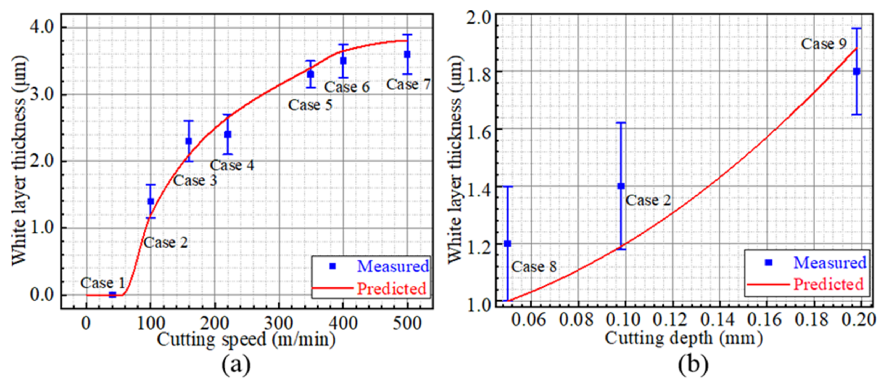
4.3. White-Layer thickness
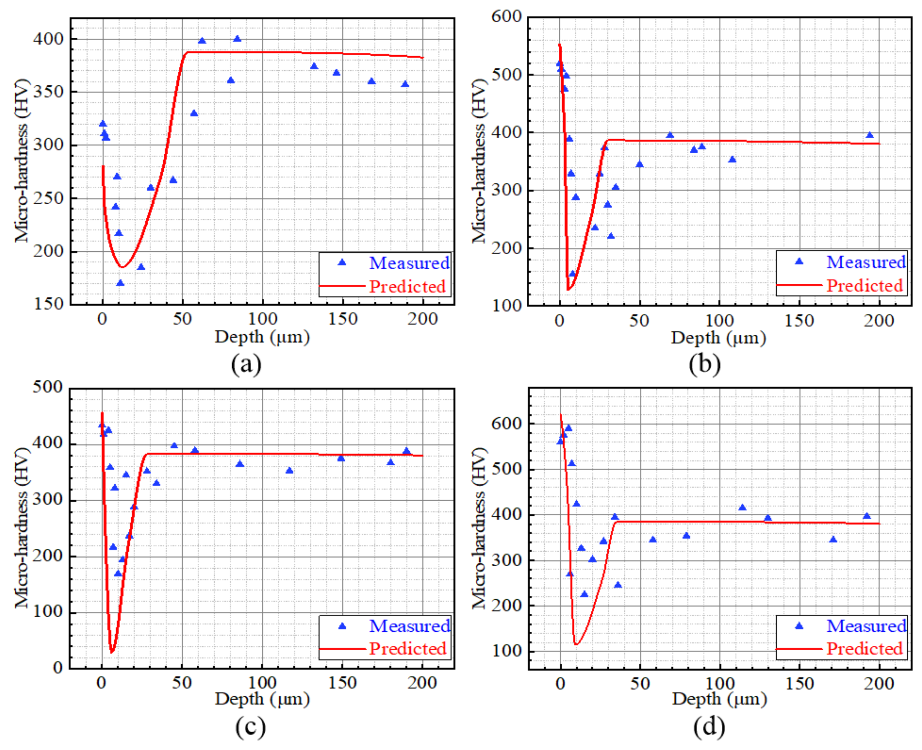
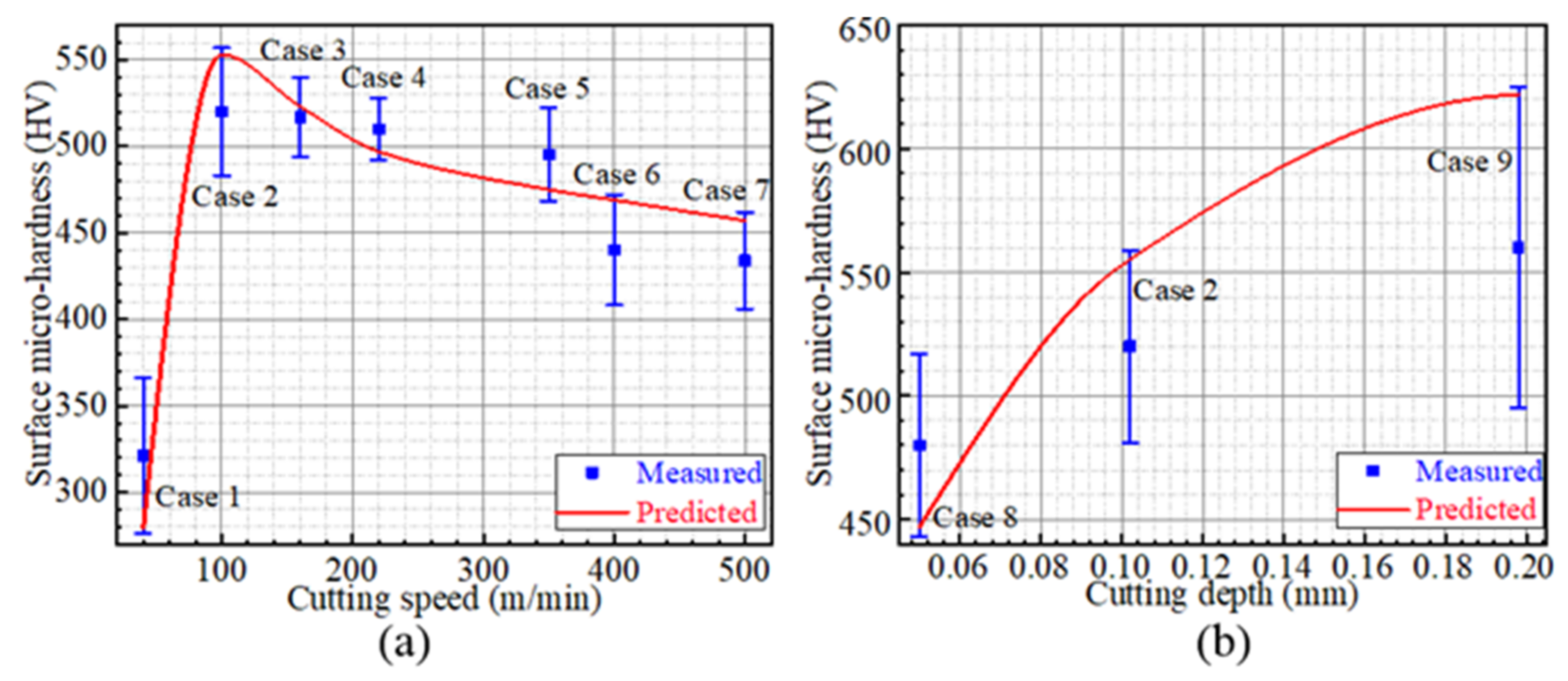
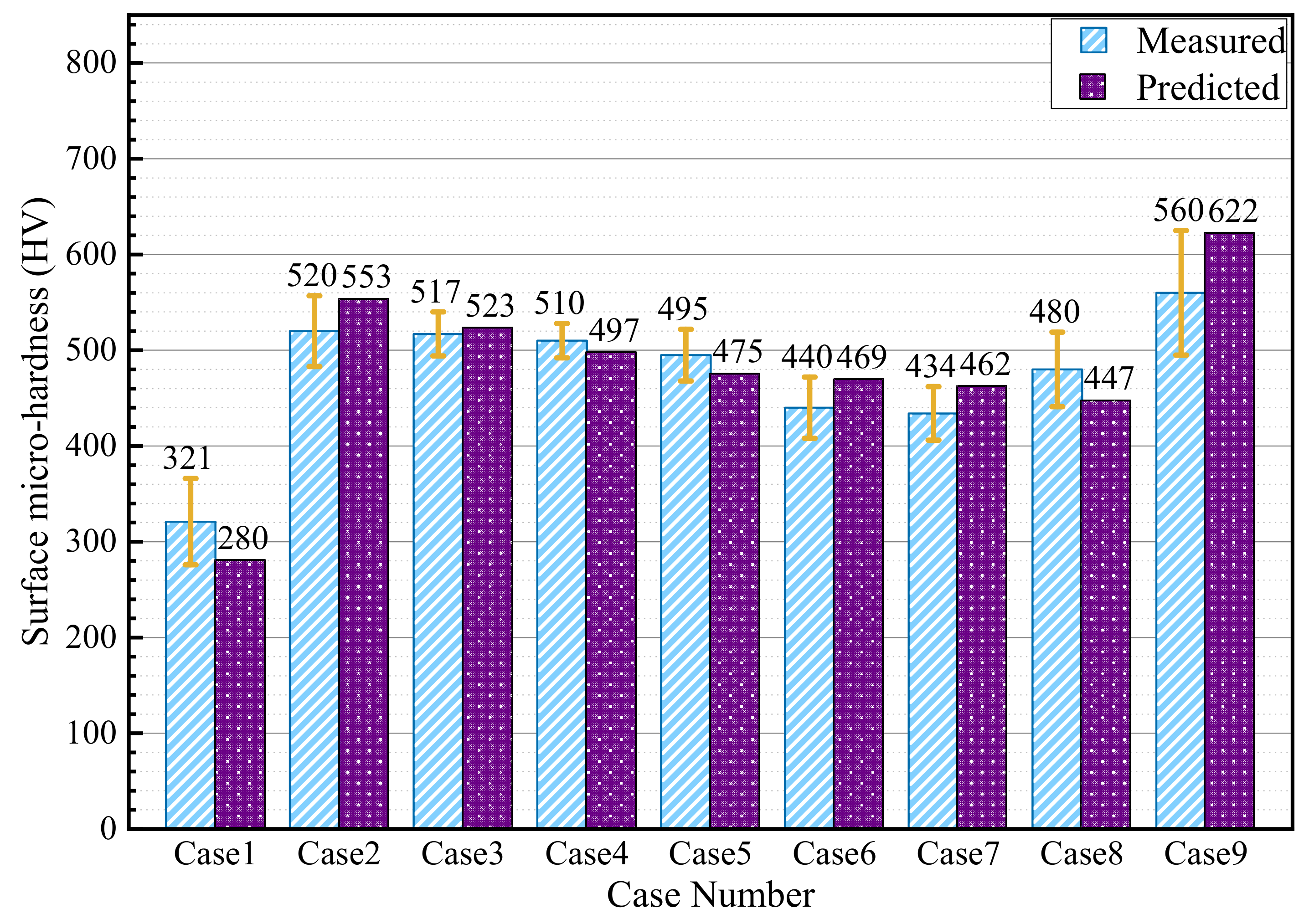
4.4. Microhardness
5. Discussion
5.1. White Layer
5.2. Microhardness
6. Conclusions
- A prediction model for white-layer thickness and microhardness is established, and the machining-induced phase transformation, white-layer generation and microhardness change can be evaluated through the variations of stress, strain and temperature. The predicted results are in good agreement with the experimental data.
- White-layer thickness is evaluated considering phase transformation and stress/strain state. There is a remarkable influence of cutting speed on the white-layer thickness since the workpiece temperature rises significantly with the increasing cutting speed.
- The microhardness change is mainly related to the dislocation density and phase transformation. The surface microhardness could be softened or hardened under different cutting conditions. The microhardness profile presents a spoon-shaped variation.
- The white-layer formation and microhardness change are highly related to cutting conditions. The present study provides a theoretical basis for controlling surface microstructure and microhardness by selecting processing parameters for industrial applications.
Author Contributions
Funding
Institutional Review Board Statement
Informed Consent Statement
Data Availability Statement
Conflicts of Interest
Nomenclature
| speed, depth, width of cut | |
| equivalent stress | |
| equivalent strain | |
| material parameters of Johnson–Cook model | |
| friction coefficient | |
| tangential force and feed force | |
| workpiece temperature, melting temperature and room temperature | |
| nominal phase-transition temperature | |
| real phase-transition temperature | |
| temperature, stress and strain fields (i, j=x, y) | |
| stress component | |
| molar volume increment and molar latent heat | |
| strain energy density | |
| equivalent plastic strain increment | |
| microhardness | |
| microhardness change due to severe plastic deformation | |
| microhardness change due to dynamic phase transformation | |
| microhardness change due to the tempering effect | |
| the magnitude of the Burgers vector of the material | |
| total dislocation density | |
| dislocation densities of cell interior and walls | |
| resolved shear-strain rates for cell interiors and walls | |
| the reference resolved shear strain | |
| the reference resolved shear-strain rate | |
| resolved shear strain | |
| resolved shear-strain rate | |
| average cell size | |
| volume fraction of the dislocation cell wall | |
| initial and saturation volume fractions of cell walls | |
| Phase-volume fraction |
References
- Ran, X.-Z.; Zhang, S.-Q.; Liu, D.; Tang, H.-B.; Wang, H.-M. Role of Microstructural Characteristics in Combination of Strength and Fracture Toughness of Laser Additively Manufactured Ultrahigh-Strength AerMet100 Steel. Metall. Mater. Trans. A 2021, 52, 1248–1259. [Google Scholar] [CrossRef]
- Zhong, J.; Yu, M.; Li, S.; Macdonald, D.D.; Xiao, B.; Liu, J. Theoretical and experimental studies of passivity breakdown of Aermet 100 ultra-high stainless steel in chloride ion medium. Mater. Corros. 2019, 70, 2020–2032. [Google Scholar] [CrossRef]
- Javaheri, V.; Sadeghpour, S.; Karjalainen, P.; Lindroos, M.; Haiko, O.; Sarmadi, N.; Pallaspuro, S.; Valtonen, K.; Pahlevani, F.; Laukkanen, A. Formation of nanostructured surface layer, the white layer, through solid particles impingement during slurry erosion in a martensitic medium-carbon steel. Wear 2022, 496, 204301. [Google Scholar] [CrossRef]
- Rajbongshi, S.K.; Sarma, D.; Singh, M.A. A Brief Review of White Layer Formation in Hard Machining with a Case Study. Adv. Mech. Eng. 2020, 407–417. [Google Scholar] [CrossRef]
- Huang, X.; Zou, F.; Ming, W.; Xu, J.; Chen, Y.; Chen, M. Wear mechanisms and effects of monolithic Sialon ceramic tools in side milling of superalloy FGH96. Ceram. Int. 2020, 46, 26813–26822. [Google Scholar] [CrossRef]
- Jawahir, I.; Brinksmeier, E.; M’saoubi, R.; Aspinwall, D.; Outeiro, J.; Meyer, D.; Umbrello, D.; Jayal, A. Surface integrity in material removal processes: Recent advances. CIRP Ann. 2011, 60, 603–626. [Google Scholar] [CrossRef]
- Madopothula, U.; Nimmagadda, R.B.; Lakshmanan, V. Assessment of white layer in hardened AISI 52100 steel and its prediction using grinding power. Mach. Sci. Technol. 2018, 22, 299–319. [Google Scholar] [CrossRef]
- Arfaoui, S.; Zemzemi, F.; Tourki, Z. A numerical-analytical approach to predict white and dark layer thickness of hard machining. Int. J. Adv. Manuf. Technol. 2018, 96, 3355–3364. [Google Scholar] [CrossRef]
- Umbrello, D.; Jawahir, I. Numerical modeling of the influence of process parameters and workpiece hardness on white layer formation in AISI 52100 steel. Int. J. Adv. Manuf. Technol. 2009, 44, 955–968. [Google Scholar] [CrossRef]
- Ranganath, S.; Guo, C.; Hegde, P. A finite element modeling approach to predicting white layer formation in nickel superalloys. CIRP Ann. 2009, 58, 77–80. [Google Scholar] [CrossRef]
- Lu, X.; Jia, Z.; Yang, K.; Shao, P.; Ruan, F.; Feng, Y.; Liang, S.Y. Analytical model of work hardening and simulation of the distribution of hardening in micro-milled nickel-based superalloy. Int. J. Adv. Manuf. Technol. 2018, 97, 3915–3923. [Google Scholar] [CrossRef]
- Chou, Y.K.; Song, H. Thermal modeling for white layer predictions in finish hard turning. Int. J. Mach. Tools Manuf. 2005, 45, 481–495. [Google Scholar] [CrossRef]
- Zhang, F.-Y.; Duan, C.-Z.; Wang, M.-J.; Sun, W. White and dark layer formation mechanism in hard cutting of AISI52100 steel. J. Manuf. Processes 2018, 32, 878–887. [Google Scholar] [CrossRef]
- Duan, C.; Zhang, F.; Sun, W.; Xu, X.; Wang, M. White layer formation mechanism in dry turning hardened steel. J. Adv. Mech. Des. Syst. Manuf. 2018, 12, JAMDSM0044. [Google Scholar] [CrossRef] [Green Version]
- Wu, S.; Liu, G.; Zhang, W.; Chen, W.; Wang, C. Formation mechanism of white layer in the high-speed cutting of hardened steel under cryogenic liquid nitrogen cooling. J. Mater. Processing Technol. 2022, 302, 117469. [Google Scholar] [CrossRef]
- Arfaoui, S.; Zemzemi, F.; Tourki, Z. Relationship between cutting process parameters and white layer thickness in orthogonal cutting. Mater. Manuf. Processes 2018, 33, 661–669. [Google Scholar] [CrossRef]
- Zhang, W.; Zhuang, K. Effect of cutting edge microgeometry on surface roughness and white layer in turning AISI 52100 steel. Procedia Cirp 2020, 87, 53–58. [Google Scholar] [CrossRef]
- Ding, H.; Shin, Y.C. Multi-physics modeling and simulations of surface microstructure alteration in hard turning. J. Mater. Processing Technol. 2013, 213, 877–886. [Google Scholar] [CrossRef]
- Pan, Z.; Liang, S.Y.; Garmestani, H.; Shih, D.S. Prediction of machining-induced phase transformation and grain growth of Ti-6Al-4 V alloy. Int. J. Adv. Manuf. Technol. 2016, 87, 859–866. [Google Scholar] [CrossRef]
- Bouissa, Y.; Zorgani, M.; Shahriari, D.; Champliaud, H.; Morin, J.-B.; Jahazi, M. Microstructure-based FEM modeling of phase transformation during quenching of large-size steel forgings. Metall. Mater. Trans. A 2021, 52, 1883–1900. [Google Scholar] [CrossRef]
- Zeng, H.; Yan, R.; Hu, T.; Du, P.; Wang, W.; Peng, F. Analytical modeling of white layer formation in orthogonal cutting of AerMet100 steel based on phase transformation mechanism. J. Manuf. Sci. Eng. 2019, 141, 064502. [Google Scholar] [CrossRef]
- Duan, C.; Kong, W.; Hao, Q.; Zhou, F. Modeling of white layer thickness in high speed machining of hardened steel based on phase transformation mechanism. Int. J. Adv. Manuf. Technol. 2013, 69, 59–70. [Google Scholar] [CrossRef]
- Zhang, W.; Wang, X.; Hu, Y.; Wang, S. Predictive modelling of microstructure changes, micro-hardness and residual stress in machining of 304 austenitic stainless steel. Int. J. Mach. Tools Manuf. 2018, 130, 36–48. [Google Scholar] [CrossRef]
- Lee, C.-H.; Chang, K.-H. Prediction of residual stresses in high strength carbon steel pipe weld considering solid-state phase transformation effects. Comput. Struct. 2011, 89, 256–265. [Google Scholar] [CrossRef]
- Grange, R.; Hribal, C.; Porter, L. Hardness of tempered martensite in carbon and low-alloy steels. Metall. Trans. A 1977, 8, 1775–1785. [Google Scholar] [CrossRef]
- Li, X.-Y.; Zhang, Z.-H.; Cheng, X.-W.; Liu, X.-P.; Zhang, S.-Z.; He, J.-Y.; Wang, Q.; Liu, L.-J. The investigation on Johnson-Cook model and dynamic mechanical behaviors of ultra-high strength steel M54. Mater. Sci. Eng. A 2022, 835, 142693. [Google Scholar] [CrossRef]
- Filice, L.; Micari, F.; Rizzuti, S.; Umbrello, D. A critical analysis on the friction modelling in orthogonal machining. Int. J. Mach. Tools Manuf. 2007, 47, 709–714. [Google Scholar] [CrossRef]
- Umbrello, D.; Hua, J.; Shivpuri, R. Hardness-based flow stress and fracture models for numerical simulation of hard machining AISI 52100 bearing steel. Mater. Sci. Eng. A 2004, 374, 90–100. [Google Scholar] [CrossRef]
- Zeng, H.; Yan, R.; Du, P.; Zhang, M.; Peng, F. Notch wear prediction model in high speed milling of AerMet100 steel with bull-nose tool considering the influence of stress concentration. Wear 2018, 408, 228–237. [Google Scholar] [CrossRef]
- Zhang, H.; Zeng, H.; Yan, R.; Wang, W.; Peng, F. Analytical modeling of cutting forces considering material softening effect in laser-assisted milling of AerMet100 steel. Int. J. Adv. Manuf. Technol. 2021, 113, 247–260. [Google Scholar] [CrossRef]
- Ding, H.; Shin, Y.C. Dislocation density-based grain refinement modeling of orthogonal cutting of titanium. J. Manuf. Sci. Eng. 2014, 136, 041003. [Google Scholar] [CrossRef]
- Mai, T.; Lim, G. Micromelting and its effects on surface topography and properties in laser polishing of stainless steel. J. Laser Appl. 2004, 16, 221–228. [Google Scholar] [CrossRef]
- Umbrello, D.; Filice, L. Improving surface integrity in orthogonal machining of hardened AISI 52100 steel by modeling white and dark layers formation. CIRP Ann. 2009, 58, 73–76. [Google Scholar] [CrossRef]
- Ghoreishi, R.; Roohi, A.H.; Ghadikolaei, A.D. Analysis of the influence of cutting parameters on surface roughness and cutting forces in high speed face milling of Al/SiC MMC. Mater. Res. Express 2018, 5, 086521. [Google Scholar] [CrossRef]


| C | Mn | Si | Ni | Cr | Mo | Al | Co | Ti | O | N | S+P | Fe |
|---|---|---|---|---|---|---|---|---|---|---|---|---|
| 0.225 | 0.01 | 0.01 | 11.22 | 3.04 | 1.20 | 0.015 | 13.50 | ≤0.015 | ≤0.002 | ≤0.0015 | 0.01 | balance |
| Thermal Conductivity (W/m·°C) | Thermal Diffusivity (m2/s) | Elastic Modulus (GPa) | Poisson’s Ratio | Yield Strength (MPa) | Tm (°C) | Tr (°C) | Density (kg/m3) | Specific Heat (J/kg·°C) |
|---|---|---|---|---|---|---|---|---|
| 19.3 | 5.9 × 10⁻⁶ | 206 | 0.3 | 831.8 | 1460 | 20 | 7889 | 412.7 |
| Case | Cutting Speed (m/min) | Cutting Depth (mm) | Cutting Width (mm) |
|---|---|---|---|
| 1 | 40 | 0.10 | 2 |
| 2 | 100 | 0.10 | 2 |
| 3 | 160 | 0.10 | 2 |
| 4 | 220 | 0.10 | 2 |
| 5 | 350 | 0.10 | 2 |
| 6 | 400 | 0.10 | 2 |
| 7 | 500 | 0.10 | 2 |
| 8 | 100 | 0.05 | 2 |
| 9 | 100 | 0.20 | 2 |
| A (MPa) | B (MPa) | C | m | n |
|---|---|---|---|---|
| 831.8 | 731.3 | 0.01 | 0.8571 | 0.2893 |
| G (GPa) | (m) | |||||||||
|---|---|---|---|---|---|---|---|---|---|---|
| 50 | 103 | 0.25 | 0.07 | 10 | 2.5 | 80 | 3.06 | 1.3 × 10¹⁰ | 1.21 × 10¹¹ | 2.48 × 10⁻¹⁰ |
Publisher’s Note: MDPI stays neutral with regard to jurisdictional claims in published maps and institutional affiliations. |
© 2022 by the authors. Licensee MDPI, Basel, Switzerland. This article is an open access article distributed under the terms and conditions of the Creative Commons Attribution (CC BY) license (https://creativecommons.org/licenses/by/4.0/).
Share and Cite
Zhang, W.; Chen, X.; Yang, C.; Wang, X.; Zhang, Y.; Li, Y.; Xue, H.; Zheng, Z. A Multiphysics Model for Predicting Microstructure Changes and Microhardness of Machined AerMet100 Steel. Materials 2022, 15, 4395. https://doi.org/10.3390/ma15134395
Zhang W, Chen X, Yang C, Wang X, Zhang Y, Li Y, Xue H, Zheng Z. A Multiphysics Model for Predicting Microstructure Changes and Microhardness of Machined AerMet100 Steel. Materials. 2022; 15(13):4395. https://doi.org/10.3390/ma15134395
Chicago/Turabian StyleZhang, Wenqian, Xupeng Chen, Chongwen Yang, Xuelin Wang, Yansong Zhang, Yongchun Li, Huan Xue, and Zhong Zheng. 2022. "A Multiphysics Model for Predicting Microstructure Changes and Microhardness of Machined AerMet100 Steel" Materials 15, no. 13: 4395. https://doi.org/10.3390/ma15134395
APA StyleZhang, W., Chen, X., Yang, C., Wang, X., Zhang, Y., Li, Y., Xue, H., & Zheng, Z. (2022). A Multiphysics Model for Predicting Microstructure Changes and Microhardness of Machined AerMet100 Steel. Materials, 15(13), 4395. https://doi.org/10.3390/ma15134395