
Concurrent Topology Optimization for Maximizing the Modal Loss Factor of Plates with Constrained Layer Damping Treatment


Abstract
:1. Introduction
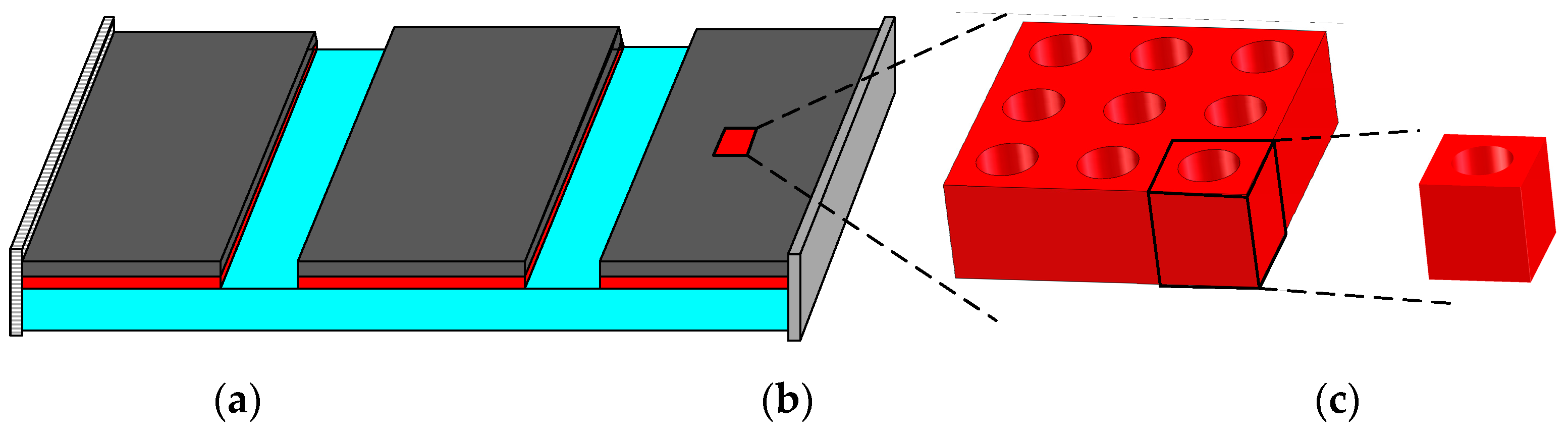
2. Multiscale CLD Structure and Its Damping Property
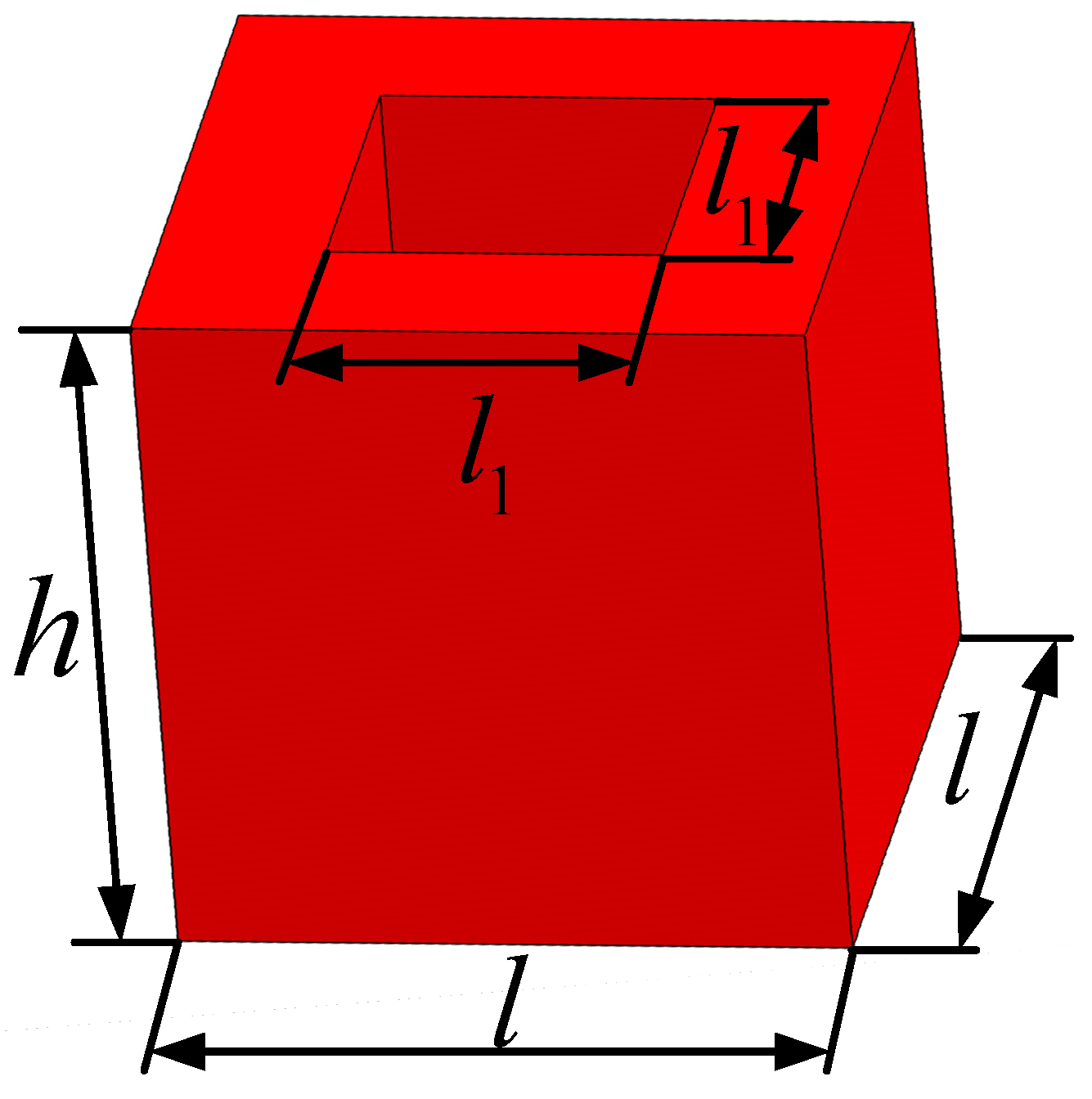
2.1. Effective Properties of Viscoelastic Damping Material
2.2. Damping Property Analysis
3. Multiscale Topology Optimization
3.1. Problem Statement and Material Interpolation Scheme
3.2. Sensitivity Analysis on the Macro Scale
3.3. Sensitivity Analysis on the Meso scale
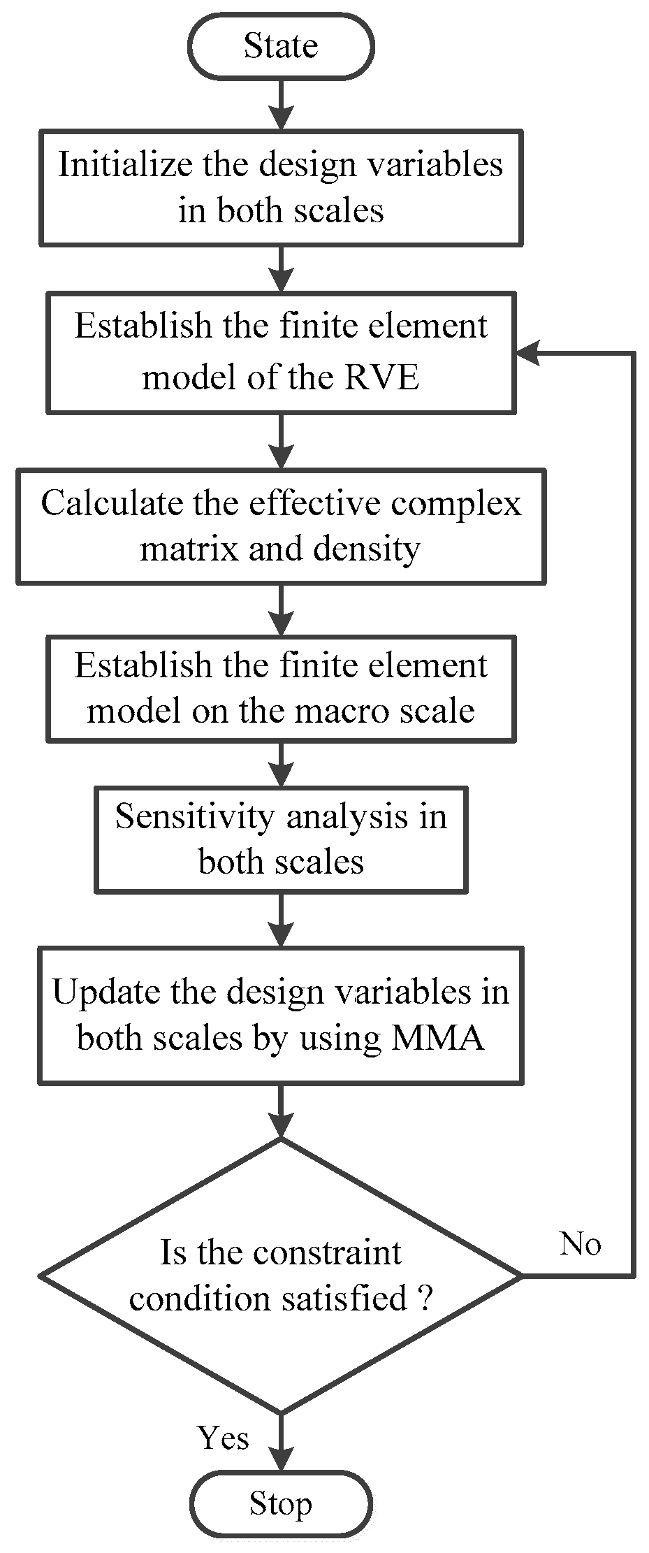
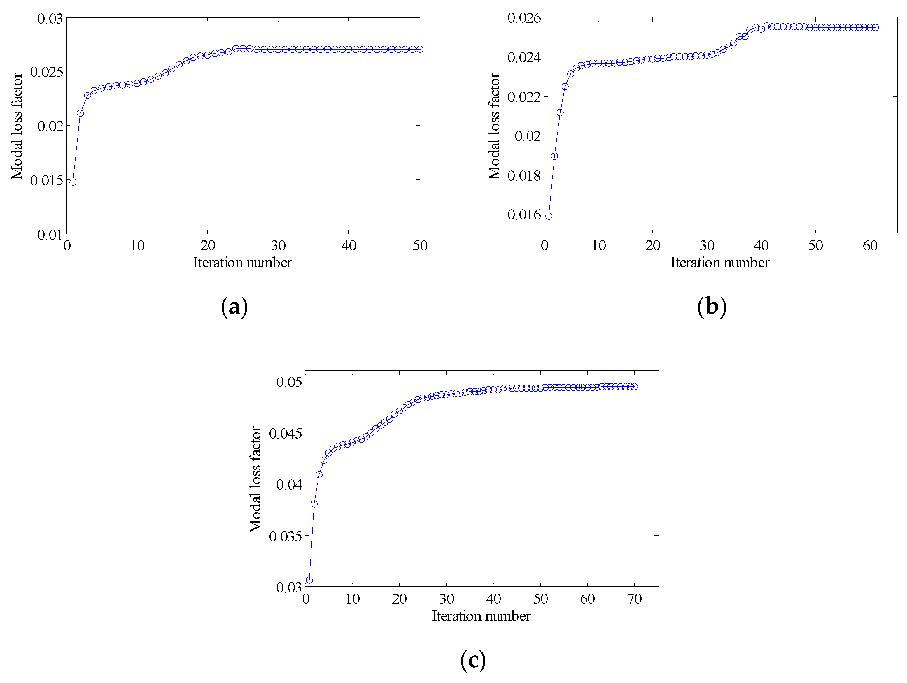
3.4. Optimization Procedure
- (1)
- Define the design domain and initialize the design variables on both scales;
- (2)
- Establish the finite element model of the RVE and calculate the effective complex matrix and density of the viscoelastic damping materials by using the RVE with a rigid skin effect;
- (3)
- Establish the finite element model on the macro scale and obtain the MLFs based on the Modal Strain Energy Method;
- (4)
- Calculate the sensitivities of the objective function with respect to the design variables on both the macro and meso scales. To circumvent the checkerboard and mesh-dependency problems, a mesh-independence filter scheme [43] was employed to smooth the element sensitivities;
- (5)
- Update the design variables on both scales by using MMA; and
- (6)
- Check the convergence of the result. If the change in the objective function of twenty successive iterations is less than , or the number of iterations reaches the preset iteration number , the iteration process terminates; otherwise, steps 2–6 are repeated.
4. Numerical Examples
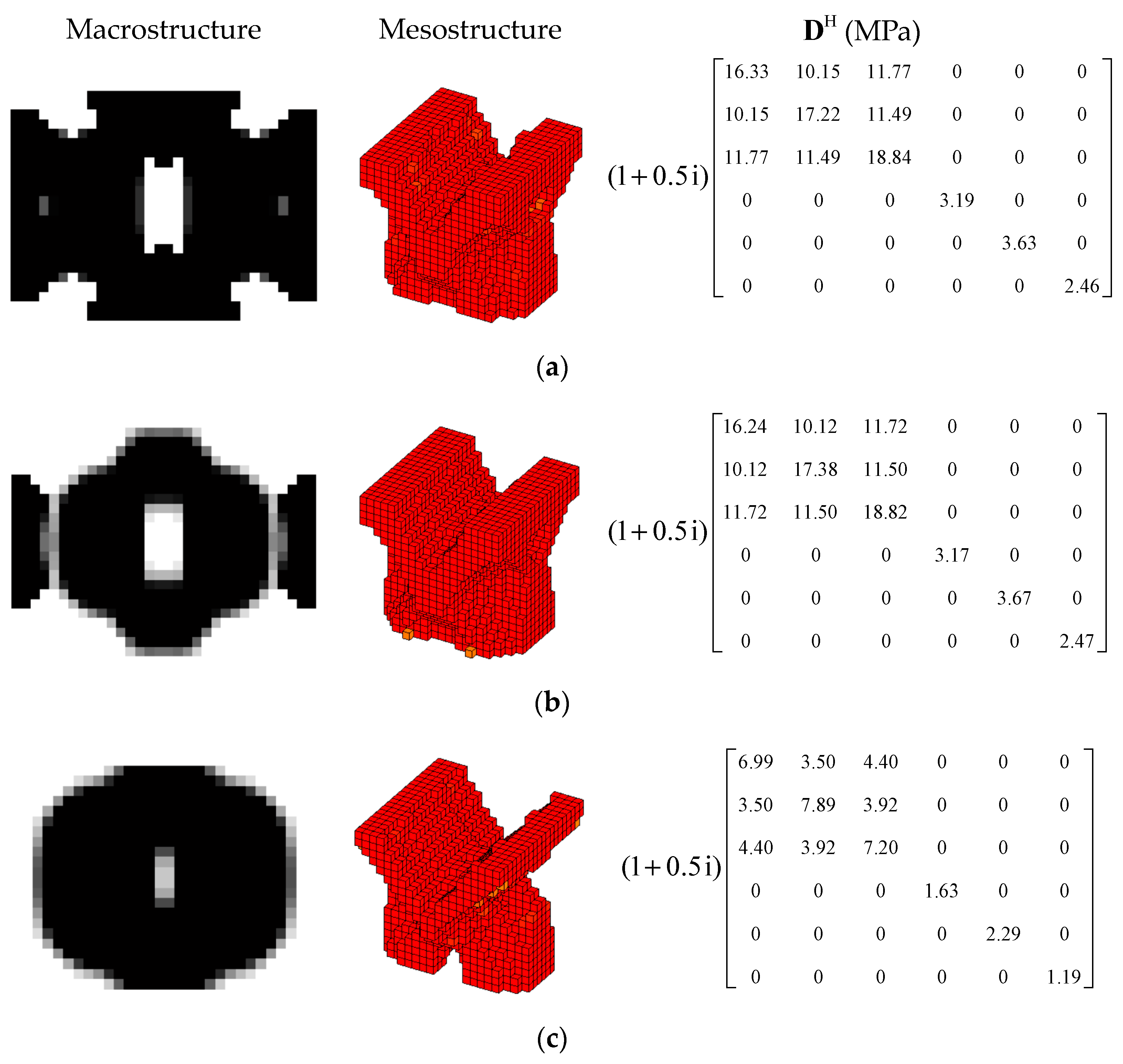
4.1. The Effective Material Property Analysis
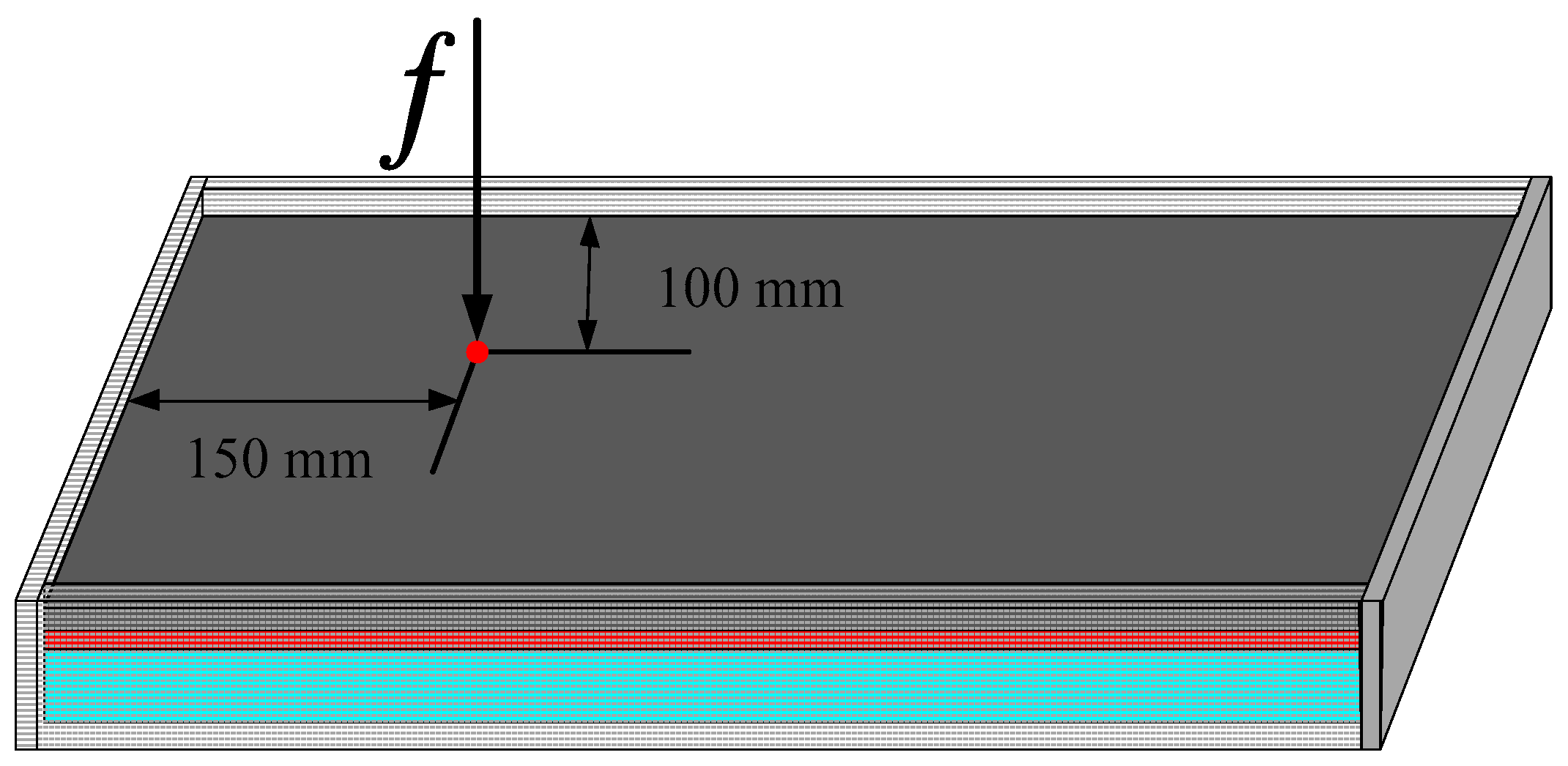
4.2. A rectangular Plate with Four Edges Clamped
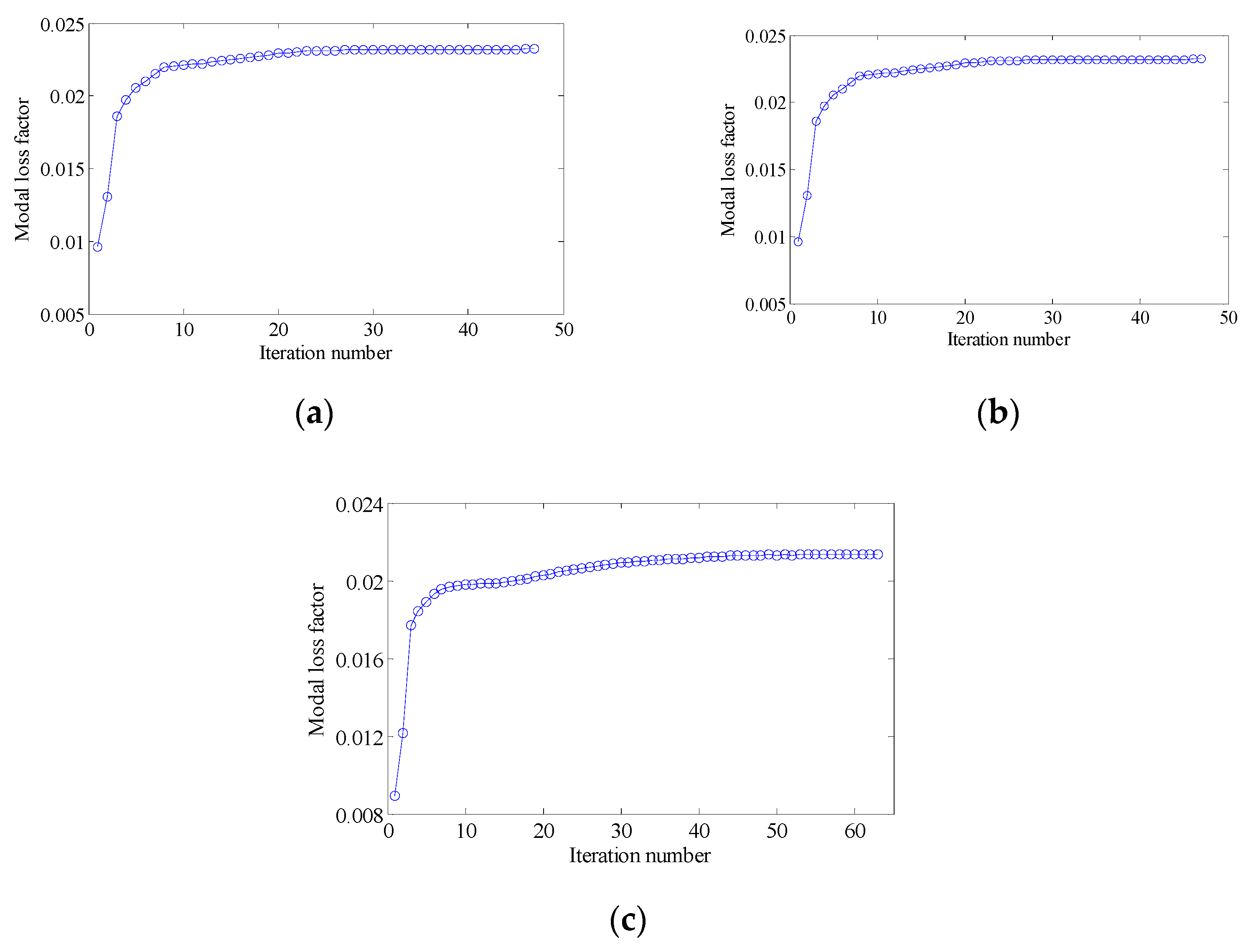
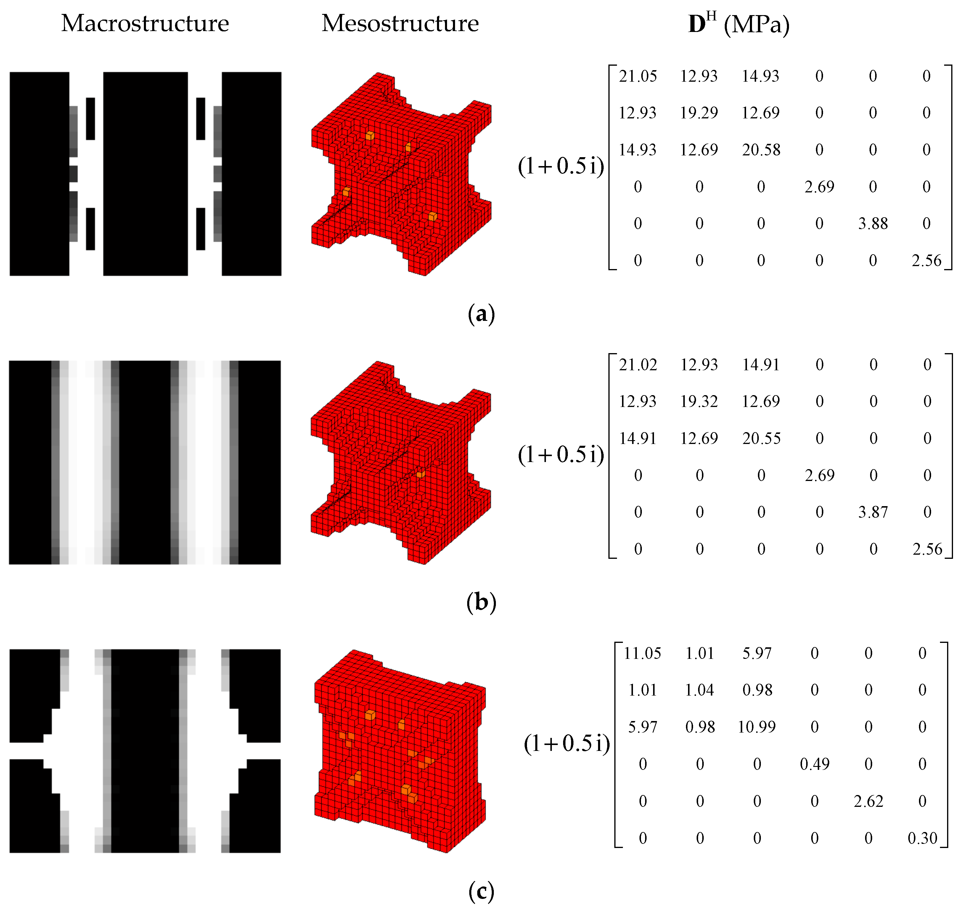
4.2.1. The Effect of Penalty Factor and Initial Guess Design on the Optimal Topologies
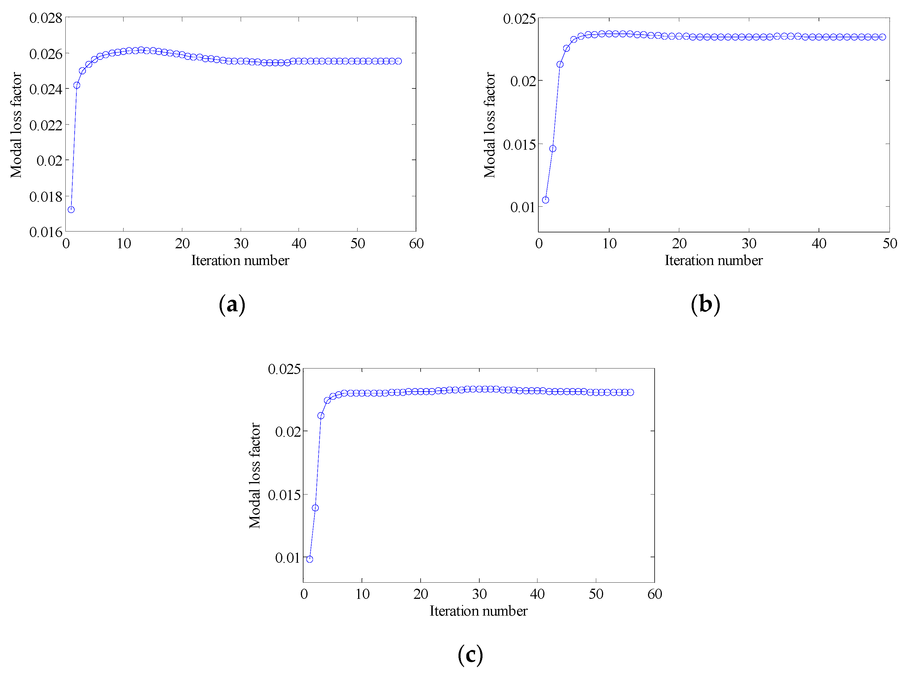
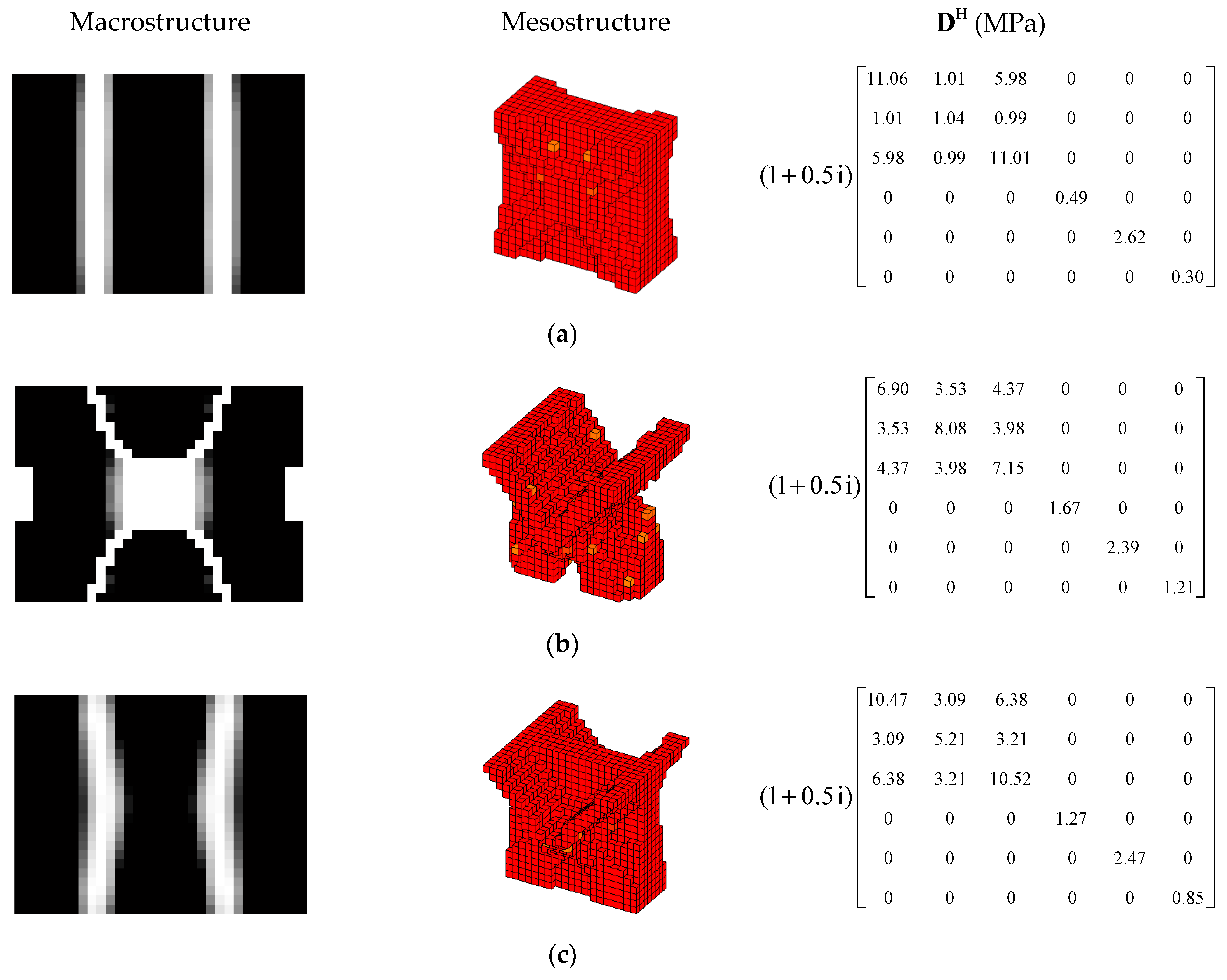
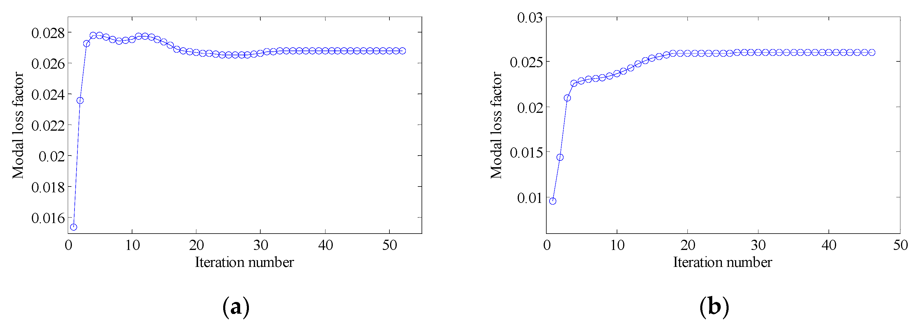
4.2.2. Different Optimization Objectives
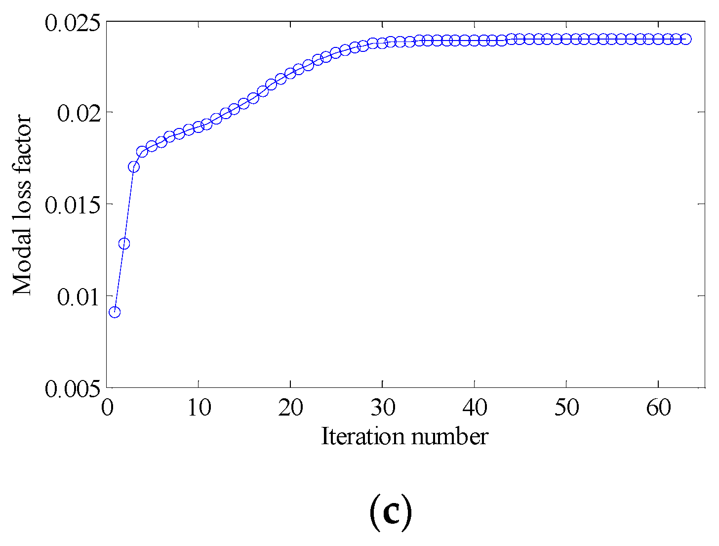
4.2.3. Different Volume Fraction
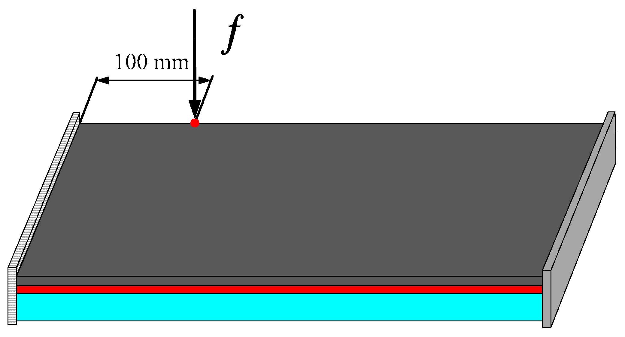
4.3. A Rectangular Plate with Two Short Edges Clamped
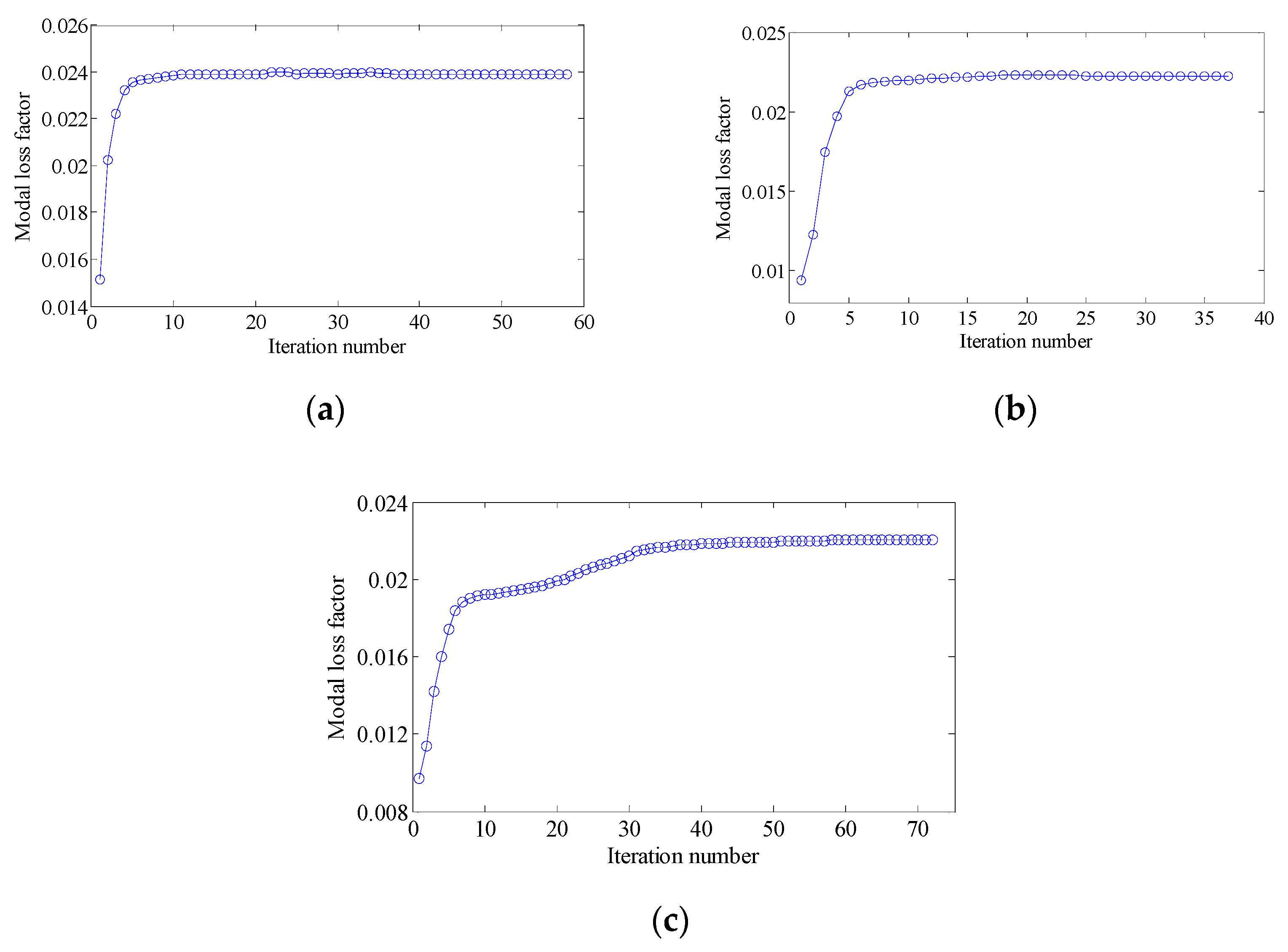
4.3.1. Different Optimization Objectives
4.3.2. Different Volume Fraction
5. Conclusions
Author Contributions
Funding
Conflicts of Interest
References
- Rao, M.D. Recent applications of viscoelastic damping for noise control in automobiles and commercial airplanes. J. Sound Vib. 2003, 262, 457–474. [Google Scholar] [CrossRef]
- Róyo, P. Optimization of i-section profile design by the finite element method. Adv. Sci. Technol. 2016, 10, 52–56. [Google Scholar]
- Ling, Z.; Ronglu, X.; Yi, W.; Elsabbagh, A. Topology Optimization of Constrained Layer Damping on Plates Using Method of Moving Asymptote (MMA) Approach. Shock. Vib. 2011, 18, 221–244. [Google Scholar] [CrossRef]
- Kim, S.Y.; Mechefske, C.K.; Kim, I.Y. Optimal damping layout in a shell structure using topology optimization. J. Sound Vib. 2013, 332, 2873–2883. [Google Scholar] [CrossRef]
- Yamamoto, T.; Yamada, T.; Izui, K.; Nishiwaki, S. Topology optimization of free-layer damping material on a thin panel for maximizing modal loss factors expressed by only real eigenvalues. J. Sound Vib. 2015, 358, 84–96. [Google Scholar] [CrossRef]
- Madeira, J.F.A.; Araújo, A.; Mota Soares, C.M. Multiobjective optimization of constrained layer damping treatments in composite plate structures. Mech. Adv. Mater. Struct. 2017, 24, 427–436. [Google Scholar] [CrossRef]
- Madeira, J.F.A.; Araújo, A.; Mota Soares, C.M.; Mota Soares, C.A. Multiobjective optimization for vibration reduction in composite plate structures using constrained layer damping. Comput. Struct. 2020, 232, 105810. [Google Scholar] [CrossRef]
- Delgado, G.; Hamdaoui, M. Topology optimization of frequency dependent viscoelastic structures via a level-set method. Appl. Math. Comput. 2019, 347, 522–541. [Google Scholar] [CrossRef] [Green Version]
- Zhang, J.; Chen, Y.; Zhai, J.; Hou, Z.; Han, Q. Topological optimization design on constrained layer damping treatment for vibration suppression of aircraft panel via improved Evolutionary Structural Optimization. Aerosp. Sci. Technol. 2021, 112, 106619. [Google Scholar] [CrossRef]
- Zhang, D.; Wu, Y.; Chen, J.; Wang, S.; Zheng, L.; Wu; Chen. Wang Sound Radiation Analysis of Constrained Layer Damping Structures Based on Two-Level Optimization. Materials 2019, 12, 3053. [Google Scholar] [CrossRef] [Green Version]
- Zhang, X.; Kang, Z. Topology optimization of damping layers for minimizing sound radiation of shell structures. J. Sound Vib. 2013, 332, 2500–2519. [Google Scholar] [CrossRef]
- Zheng, W.; Yang, T.; Huang, Q.; He, Z. Topology optimization of PCLD on plates for minimizing sound radiation at low frequency resonance. Struct. Multidiscip. Optim. 2016, 53, 1231–1242. [Google Scholar] [CrossRef]
- Takezawa, A.; Daifuku, M.; Nakano, Y.; Nakagawa, K.; Yamamoto, T.; Kitamura, M. Topology optimization of damping material for reducing resonance response based on complex dynamic compliance. J. Sound Vib. 2016, 365, 230–243. [Google Scholar] [CrossRef] [Green Version]
- Li, M.; Li, C. Topological optimization of damping layout for minimized sound radiation of an acoustic black hole plate. J. Sound Vib. 2019, 458, 349–364. [Google Scholar]
- Zhang, Z.; Chen, W. An approach for topology optimization of damping layer under harmonic excitations based on piecewise constant level set method. J. Comput. Phys. 2019, 390, 470–489. [Google Scholar] [CrossRef]
- Chen, W.; Liu, S. Topology optimization of microstructures of viscoelastic damping materials for a prescribed shear modulus. Struct. Multidiscip. Optim. 2014, 50, 287–296. [Google Scholar] [CrossRef]
- Sigmund, O. Materials with prescribed constitutive parameters: An inverse homogenization problem. Int. J. Solids Struct. 1994, 31, 2313–2329. [Google Scholar] [CrossRef]
- Sigmund, O. Tailoring materials with prescribed elastic properties. Mech. Mater. 1995, 20, 351–368. [Google Scholar] [CrossRef]
- Huang, X.; Zhou, S.; Sun, G.; Li, G.; Xie, Y.M. Topology optimization for microstructures of viscoelastic composite materials. Comput. Methods Appl. Mech. Eng. 2015, 283, 503–516. [Google Scholar] [CrossRef]
- Chen, W.; Liu, S. Microstructural topology optimization of viscoelastic materials for maximum modal loss factor of macrostructures. Struct. Multidiscip. Optim. 2016, 53, 1–14. [Google Scholar] [CrossRef]
- Asadpoure, A.; Tootkaboni, M.; Valdevit, L. Topology optimization of multiphase architected materials for energy dissipation. Comput. Methods Appl. Mech. Eng. 2017, 325, 314–329. [Google Scholar] [CrossRef]
- Yun, K.S.; Youn, S.K. Microstructural topology optimization of viscoelastic materials of damped structures subjected to dynamic loads. Int. J. Solids Struct. 2018, 147, 67–79. [Google Scholar] [CrossRef]
- Liu, Q.; Ruan, D.; Huang, X. Topology optimization of viscoelastic materials on damping and frequency of macrostructures. Comput. Methods Appl. Mech. Eng. 2018, 337, 305–323. [Google Scholar] [CrossRef]
- Giraldo-Londoo, O.; Paulino, G.H. Fractional topology optimization of periodic multi-material viscoelastic microstructures with tailored energy dissipation. Comput. Methods Appl. Mech. Eng. 2020, 372, 113307. [Google Scholar] [CrossRef]
- Zhang, H.; Ding, X.; Wang, Q.; Ni, W.; Li, H. Topology optimization of composite material with high broadband damping. Comput. Struct. 2020, 239, 106331. [Google Scholar] [CrossRef]
- Tsumura, K. Hierarchically Aggregated Optimization Algorithm for Heterogeneously Dispersed Utility Functions. IFAC-PapersOnLine 2017, 50, 14442–14446. [Google Scholar] [CrossRef]
- Niu, B.; Yan, J.; Cheng, G. Optimum structure with homogeneous optimum cellular material for maximum fundamental frequency. Struct. Multidiscip. Optim. 2009, 39, 115–132. [Google Scholar] [CrossRef]
- Zuo, Z.H.; Huang, X.; Rong, J.H.; Xie, Y.M. Multi-scale design of composite materials and structures for maximum natural frequencies. Mater. Des. 2013, 51, 1023–1034. [Google Scholar] [CrossRef]
- Coelho, P.; Guedes, J.; Rodrigues, H. Multiscale topology optimization of bi-material laminated composite structures. Compos. Struct. 2015, 132, 495–505. [Google Scholar] [CrossRef]
- Zhang, Y.; Xiao, M.; Li, H.; Gao, L.; Chu, S. Multiscale concurrent topology optimization for cellular structures with multiple microstructures based on ordered SIMP interpolation. Comput. Mater. Sci. 2018, 155, 74–91. [Google Scholar] [CrossRef]
- Gao, J.; Luo, Z.; Li, H.; Gao, L. Topology optimization for multiscale design of porous composites with multi-domain microstructures. Comput. Methods Appl. Mech. Eng. 2019, 344, 451–476. [Google Scholar] [CrossRef]
- Hoang, V.-N.; Tran, P.; Vu, V.-T.; Nguyen-Xuan, H. Design of lattice structures with direct multiscale topology optimization. Compos. Struct. 2020, 252, 112718. [Google Scholar] [CrossRef]
- Zhang, Y.; Xiao, M.; Gao, L.; Gao, J.; Li, H. Multiscale topology optimization for minimizing frequency responses of cellular composites with connectable graded microstructures. Mech. Syst. Signal Process. 2020, 135, 106369. [Google Scholar] [CrossRef]
- Zhang, H.; Ding, X.; Li, H.; Xiong, M. Multi-scale structural topology optimization of free-layer damping structures with damping composite materials. Compos. Struct. 2019, 212, 609–624. [Google Scholar] [CrossRef]
- Sorohan, S.; Constantinescu, D.M.; Sandu, M.; Sandu, A.G. On the homogenization of hexagonal honeycombs under axial and shear loading. Part II: Comparison of free skin and rigid skin effects on effective core properties. Mech. Mater. 2017, 119, 92–108. [Google Scholar] [CrossRef]
- Attipou, K.; Nezamabadi, S.; Daya, E.M.; Zahrouni, H. A multiscale approach for the vibration analysis of heterogeneous materials: Application to passive damping. J. Sound Vib. 2013, 332, 725–739. [Google Scholar] [CrossRef] [Green Version]
- Sorohan, S.; Constantinescu, D.M.; Sandu, M.; Sandu, A.G. On the homogenization of hexagonal honeycombs under axial and shear loading. Part I: Analytical formulation for free skin effect, Mech. Mater. 2017, 119, 74–91. [Google Scholar]
- Cristescu, N.D.; Craciun, E.M.; Soós, E. Mechanics of Elastic Composites; Chapman & Hall/CRC Press: Boca Raton, FL, USA, 2003. [Google Scholar]
- Chwa, M.; Muc, A. Design of reinforcement in nano- and microcomposites. Materials 2019, 12, 1474. [Google Scholar] [CrossRef] [Green Version]
- Hohe, J.; Becker, W. A refined analysis of the effective elasticity tensor for general cellular sandwich cores. Int. J. Solids Struct. 2001, 38, 3689–3717. [Google Scholar] [CrossRef]
- Stolpe, M.; Svanberg, K. An interpolation model for minimum compliance topology optimization. Struct. Multidiscip. Optim. 2001, 22, 116–124. [Google Scholar] [CrossRef]
- Zhang, D.; Wu, Y.; Lu, X.; Zheng, L. Topology optimization of constrained layer damping plates with frequency- and temperature-dependent viscoelastic core via parametric level set method. Mech. Adv. Mater. Struct. 2021, 29, 1938302. [Google Scholar] [CrossRef]
- Sigmund, O. On the Design of Compliant Mechanisms Using Topology Optimization. Mech. Struct. Mach. 1997, 25, 493–524. [Google Scholar] [CrossRef]
- Marin, M.; Craciun, E.M.; Pop, N. Some Results in Green–Lindsay Thermoelasticity of Bodies with Dipolar Structure. Mathematics 2020, 8, 497. [Google Scholar] [CrossRef] [Green Version]
- Xia, L.; Breitkopf, P. Multiscale structural topology optimization with an approximate constitutive model for local material microstructure. Comput. Methods Appl. Mech. Eng. 2015, 286, 147–167. [Google Scholar] [CrossRef]


| 1st Load Case | 2nd Load Case | 3rd Load Case | |||||||||
| Nodes | Nodes | Nodes | |||||||||
| X = 0 | 0 | Free | Free | X = 0 | 0 | Free | Free | X = 0 | 0 | Free | Free |
| X = a | Free | Free | X = a | 0 | Free | Free | X = a | 0 | Free | Free | |
| Y = 0 | Free | 0 | Free | Y = 0 | Free | 0 | Free | Y = 0 | Free | 0 | Free |
| Y = b | Free | 0 | Free | Y = b | Free | Free | Y = b | Free | 0 | Free | |
| Z = 0 | Free | Free | 0 | Z = 0 | Free | Free | 0 | Z = 0 | Free | Free | 0 |
| Z = c | 0 | 0 | Z = c | 0 | 0 | Z = c | 0 | 0 | |||
| 4th load case | 5th Load Case | 6th Load Case | |||||||||
| Nodes | Nodes | Nodes | |||||||||
| X = 0 | 0 | Free | Free | X = 0 | Free | 0 | 0 | X = 0 | Free | 0 | 0 |
| X = a | 0 | Free | Free | X = a | Free | 0 | 0 | X = a | Free | 0 | 0 |
| Y = 0 | 0 | Free | 0 | Y = 0 | Free | 0 | Free | Y = 0 | 0 | Free | 0 |
| Y = b | 0 | Free | 0 | Y = b | Free | 0 | Free | Y = b | Free | 0 | |
| Z = 0 | 0 | 0 | Free | Z = 0 | 0 | 0 | Free | Z = 0 | Free | Free | 0 |
| Z = c | 0 | 0 | Z = c | 0 | 0 | Z = c | 0 | 0 | |||
| 7th load case | 8th load case | 9th load case | |||||||||
| Nodes | Nodes | Nodes | |||||||||
| X = 0 | 0 | Free | Free | X = 0 | 0 | Free | Free | X = 0 | 0 | Free | Free |
| X = a | Free | Free | X = a | Free | Free | X = a | 0 | Free | Free | ||
| Y = 0 | Free | 0 | Free | Y = 0 | Free | 0 | Free | Y = 0 | Free | 0 | Free |
| Y = b | Free | Free | Y = b | Free | 0 | Free | Y = b | Free | Free | ||
| Z = 0 | Free | Free | 0 | Z = 0 | Free | Free | 0 | Z = 0 | Free | Free | 0 |
| Z = c | 0 | Z = c | 0 | Z = c | 0 | ||||||
| Layer | Density (kg/m3) | Young’s Modulus (MPa) | Poisson’s Ratio | Material Loss Factor |
|---|---|---|---|---|
| Base plate, | 7900 | 0.3 | —— | |
| Viscoelastic layer | 1200 | 20 | 0.495 | 0.5 |
| Constrained layer | 2800 | 0.3 | —— |
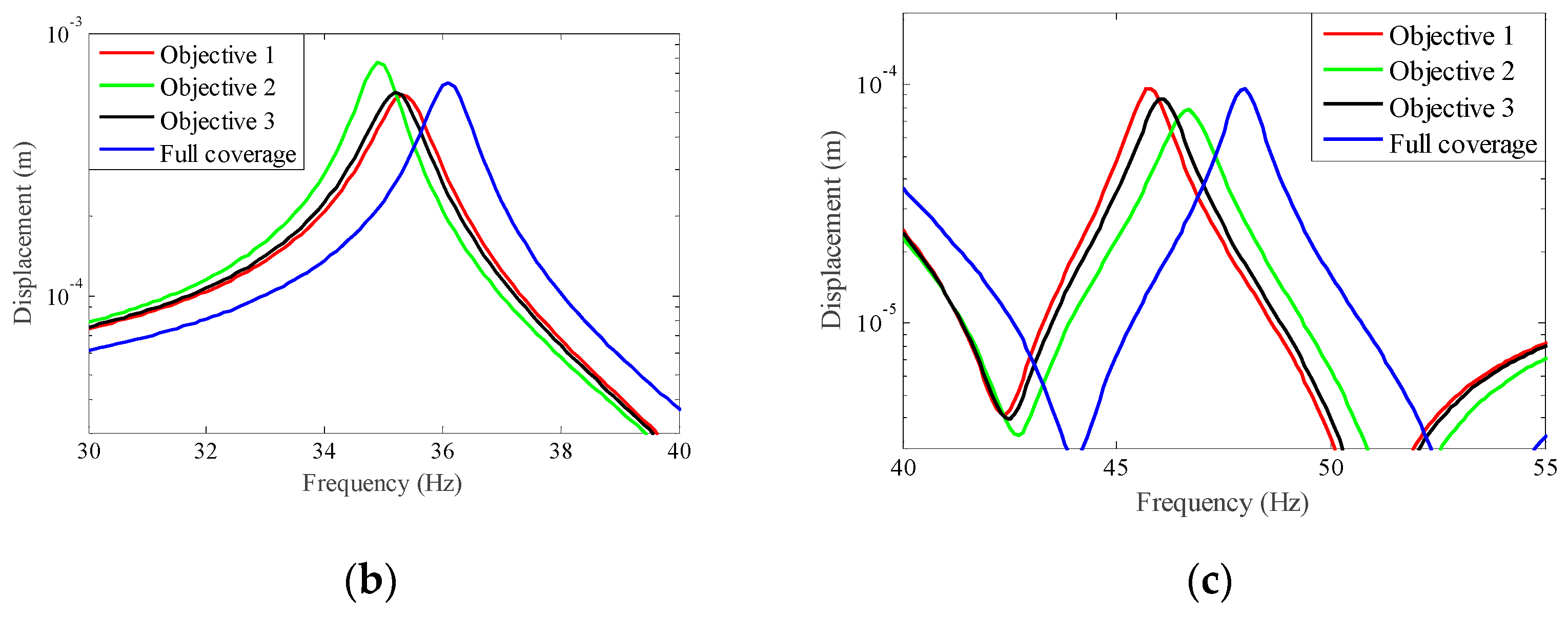
| Objective 1 | Objective 2 | Objective 3 | Full Coverage Structure | |
|---|---|---|---|---|
| The first modal loss factor | 0.024 | 0.019 | 0.023 | 0.023 |
| The second modal loss factor | 0.022 | 0.026 | 0.026 | 0.024 |
| The sum of the first two modal loss factors | 0.046 | 0.045 | 0.049 | 0.047 |
| The Optimum Design for Maximizing the First Modal Loss Factor | The Optimum Design for Maximizing the Second Modal Loss Factor | |||||
|---|---|---|---|---|---|---|
| Case 1 | Case 2 | Case 3 | Case 4 | Case 5 | Case 6 | |
| The first modal loss factor | 0.025 | 0.023 | 0.022 | 0.019 | 0.012 | 0.013 |
| The second modal loss factor | 0.021 | 0.018 | 0.019 | 0.026 | 0.023 | 0.023 |
| Objective 1 | Objective 2 | Objective 3 | Full Coverage Structure | |
|---|---|---|---|---|
| The first modal loss factor | 0.027 | 0.021 | 0.027 | 0.023 |
| The second modal loss factor | 0.021 | 0.025 | 0.023 | 0.019 |
| The sum of the first two modal loss factors | 0.048 | 0.046 | 0.050 | 0.042 |
| The Optimum Design for Maximizing the First Modal Loss Factor | The Optimum Design for Maximizing the Second Modal Loss Factor | |||||
|---|---|---|---|---|---|---|
| Case 1 | Case 2 | Case 3 | Case 4 | Case 5 | Case 6 | |
| The first modal loss factor | 0.027 | 0.026 | 0.024 | 0.021 | 0.019 | 0.017 |
| The second modal loss factor | 0.023 | 0.019 | 0.017 | 0.024 | 0.022 | 0.022 |
Publisher’s Note: MDPI stays neutral with regard to jurisdictional claims in published maps and institutional affiliations. |
© 2022 by the authors. Licensee MDPI, Basel, Switzerland. This article is an open access article distributed under the terms and conditions of the Creative Commons Attribution (CC BY) license (https://creativecommons.org/licenses/by/4.0/).
Share and Cite
Fang, Z.; Yao, L.; Hou, J.; Xiao, Y. Concurrent Topology Optimization for Maximizing the Modal Loss Factor of Plates with Constrained Layer Damping Treatment. Materials 2022, 15, 3512. https://doi.org/10.3390/ma15103512
Fang Z, Yao L, Hou J, Xiao Y. Concurrent Topology Optimization for Maximizing the Modal Loss Factor of Plates with Constrained Layer Damping Treatment. Materials. 2022; 15(10):3512. https://doi.org/10.3390/ma15103512
Chicago/Turabian StyleFang, Zhanpeng, Lei Yao, Junjian Hou, and Yanqiu Xiao. 2022. "Concurrent Topology Optimization for Maximizing the Modal Loss Factor of Plates with Constrained Layer Damping Treatment" Materials 15, no. 10: 3512. https://doi.org/10.3390/ma15103512
APA StyleFang, Z., Yao, L., Hou, J., & Xiao, Y. (2022). Concurrent Topology Optimization for Maximizing the Modal Loss Factor of Plates with Constrained Layer Damping Treatment. Materials, 15(10), 3512. https://doi.org/10.3390/ma15103512