
A Versatile Punch Stroke Correction Model for Trial V-Bending of Sheet Metals Based on Data-Driven Method

 ,
,
Abstract
:1. Introduction
2. Research Methods
2.1. Modeling Principle
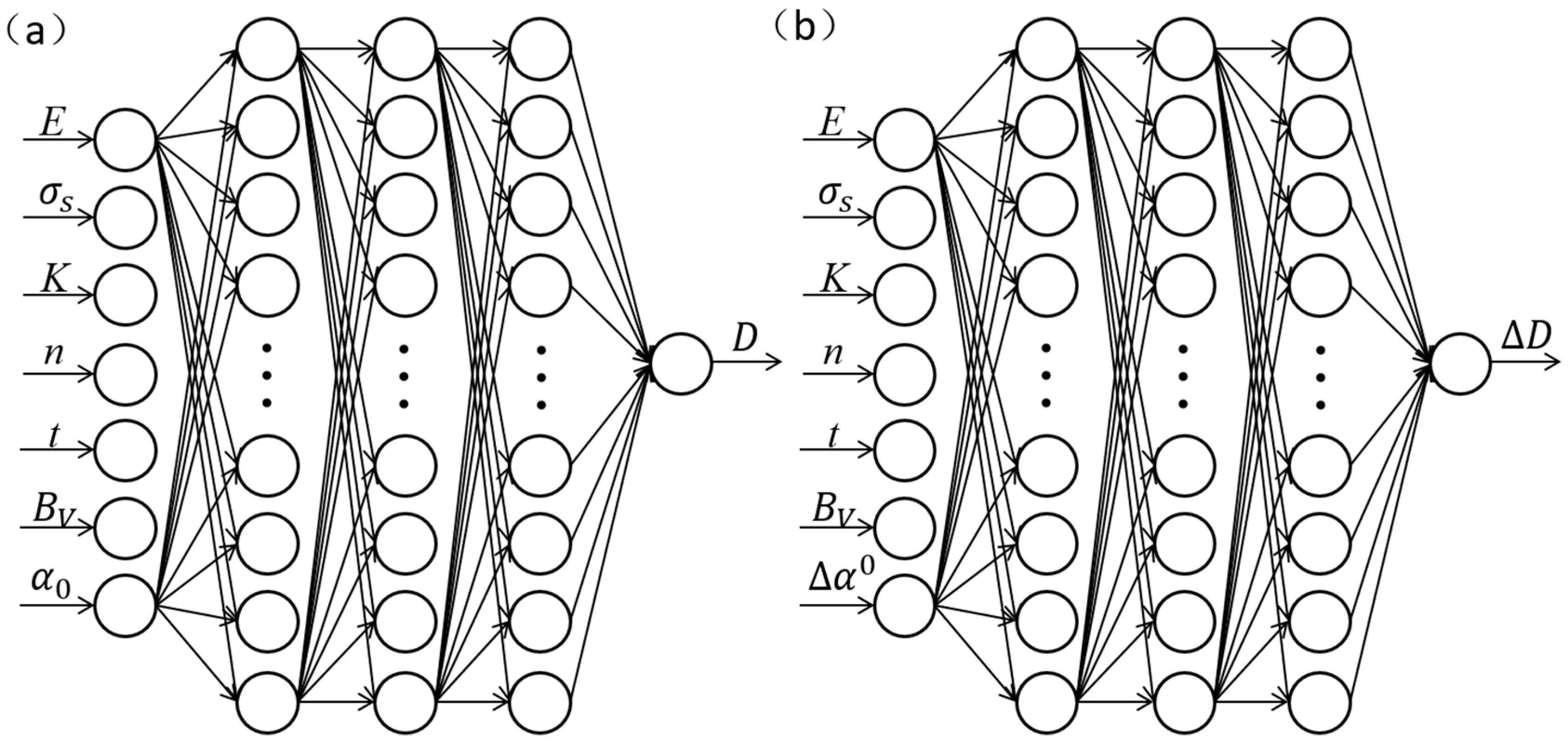
2.1.1. GA–BPNN Model
- (1)
- Forward propagation of signals
- (2)
- Backpropagation
2.1.2. Mathematical Model of Dimensional Analysis
2.2. Sample Range Definition for Dataset
2.3. Acquisition of Finite Element Sample for Training Data
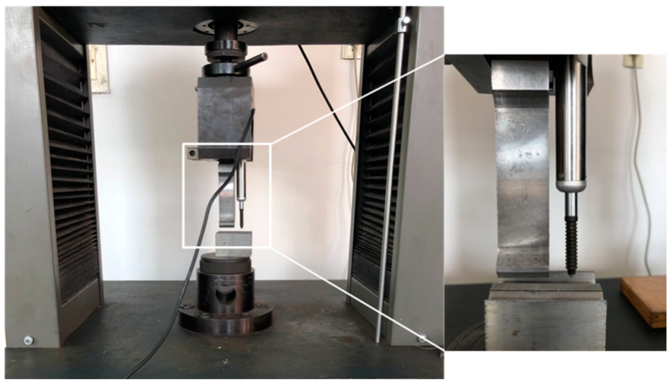
2.4. Mechanical Tests and Bending Tests
2.5. Data Acquisition for the Correction Model
3. Results and Analysis
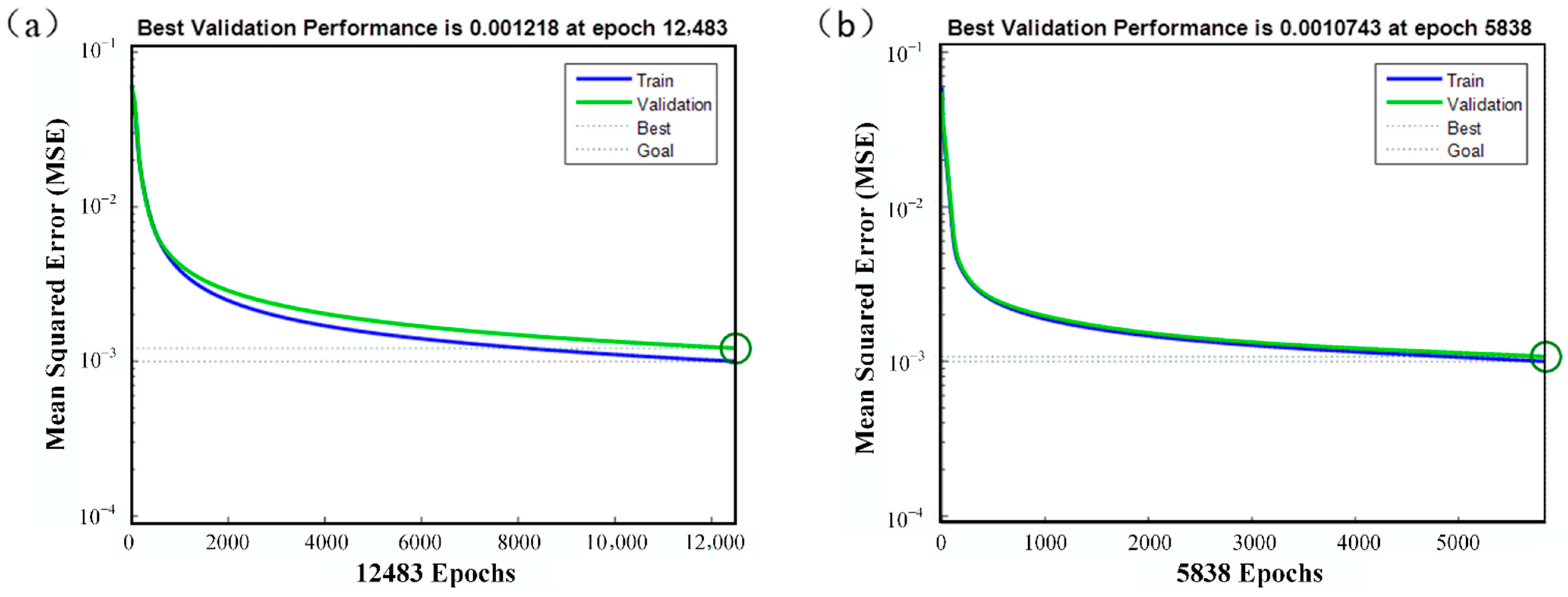
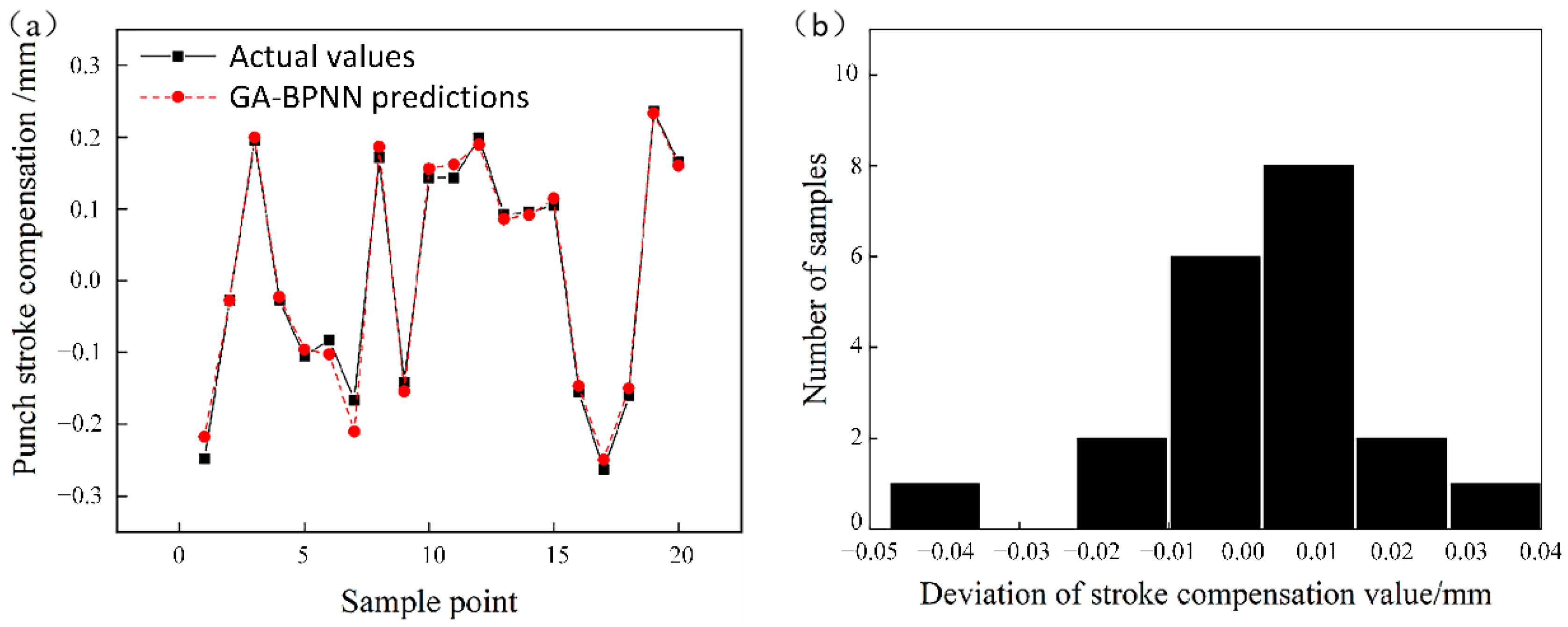
3.1. Punch Stroke Correction Model Based on a GA-BPNN
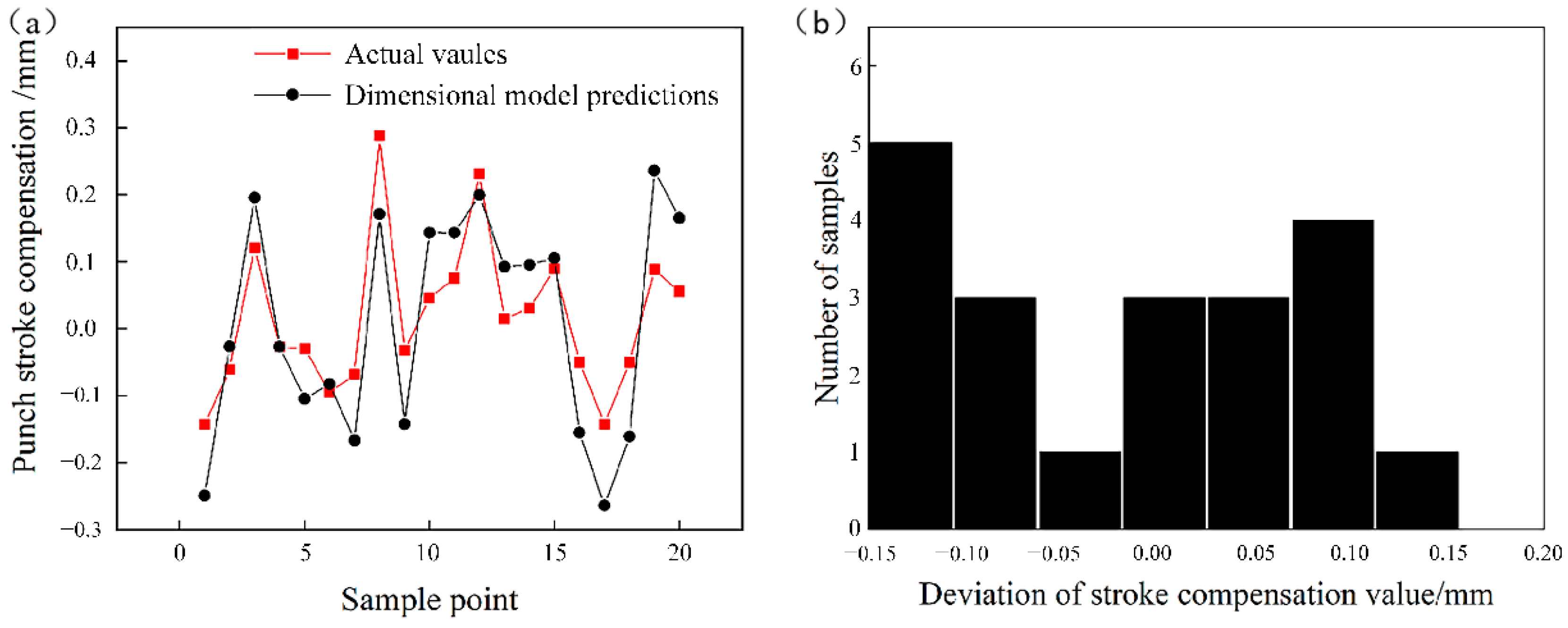
3.2. Punch Stroke Correction Model Based on Dimensional Analysis
3.3. Application Examples
4. Conclusions
- (1)
- A large sample dataset was established via finite element method for bending experiments using various sheet metals. Based on the dataset, a GA-BPNN prediction model was established, whose accuracy was guaranteed within 0.16 mm by the contrast with actual bending experiments;
- (2)
- In order to further improve the accuracy of the model-guided processing, the GA-BPNN and dimensional analysis were used for the establishment of the correction model. By comparing the verification results with the targets in the dataset, the GA-BPNN correction model was more capable of fitting the target problem, and the deviation of punch stroke compensation could be controlled within 0.05 mm;
- (3)
- The accuracy of the GA-BPNN punch stroke prediction model and the GA-BPNN punch stroke correction model was verified via bending experiments using a universal material testing machine. Calculated by the prediction model once and the correction model two times, the error of all of the forming angles could be less than 0.5°. Our work provides a new method to solve the problem of precise rapid forming in sheet metal bending.
Author Contributions
Funding
Institutional Review Board Statement
Informed Consent Statement
Data Availability Statement
Conflicts of Interest
References
- Leu, D.K. Position deviation and springback in V-die bending process with asymmetric dies. Int. J. Adv. Manuf. Technol. 2015, 79, 1095–1108. [Google Scholar] [CrossRef]
- Wagoner, R.H.; Lim, H.; Lee, M.-G. Advanced Issues in springback. Int. J. Plast. 2013, 45, 3–20. [Google Scholar] [CrossRef]
- Li, F.; Wu, J.; Li, Y.; Zhang, Z.; Wang, Y.A. A new calculating method to perform springback predictions for varied curvature sheet bending based on the B-spline function. Int. J. Mech. Sci. 2016, 113, 71–80. [Google Scholar] [CrossRef]
- Zajkani, A.; Hajbarati, H. An analytical modeling for springback prediction during U-bending process of advanced high-strength steels based on anisotropic nonlinear kinematic hardening model. Int. J. Adv. Manuf. Technol. 2017, 90, 349–359. [Google Scholar] [CrossRef]
- Liu, W.J.; Liu, Q.; Ruan, F.; Liang, Z.Y.; Qiu, H.Y. Springback prediction for sheet metal forming based on GA-ANN technology. J. Mater. Process. Technol. 2007, 187, 227–231. [Google Scholar] [CrossRef]
- Trzepiecinski, T.; Lemu, H.G. Improving Prediction of Springback in Sheet Metal Forming Using Multilayer Perceptron-Based Genetic Algorithm. Materials 2020, 13, 16. [Google Scholar] [CrossRef]
- Zafer, T. An experimental study on the examination of springback of sheet metals with several thicknesses and properties in bending dies. J. Mater. Process. Technol. 2004, 145, 109–177. [Google Scholar] [CrossRef]
- Li, Y.; Liang, Z.; Zhang, Z.; Zou, T.; Li, D.; Ding, S.; Xiao, H.; Shi, L. An analytical model for rapid prediction and compensation of springback for chain-die forming of an AHSS U-channel. Int. J. Mech. Sci. 2019, 159, 195–212. [Google Scholar] [CrossRef]
- Zhan, M.; Xing, L.; Gao, P.F.; Ma, F. An analytical springback model for bending of welded tube considering the weld characteristics. Int. J. Mech. Sci. 2019, 150, 594–609. [Google Scholar] [CrossRef]
- Jamli, M.R.; Ariffin, A.K.; Wahab, D.A. Integration of feedforward neural network and finite element in the draw-bend springback prediction. Expert Syst. Appl. 2014, 41, 3662–3670. [Google Scholar] [CrossRef]
- Asl, Y.D.; Woo, Y.Y.; Kim, Y.; Moon, Y.H. Non-sorting multi-objective optimization of flexible roll forming using artificial neural networks. Int. J. Adv. Manuf. Technol. 2020, 107, 2875–2888. [Google Scholar] [CrossRef]
- Kurtaran, H. A novel approach for the prediction of bend allowance in air bending and comparison with other methods. Int. J. Adv. Manuf. Technol. 2008, 37, 486–495. [Google Scholar] [CrossRef]
- Vorkov, V.; García, A.T.; Rodrigues, G.C.; Duflou, J.R. Data-driven prediction of air bending. Procedia Manuf. 2019, 29, 177–184. [Google Scholar] [CrossRef]
- Dalzochio, J.; Kunst, R.; Pignaton, E.; Binotto, A.; Sanyal, S.; Favilla, J.; Barbosa, J. Machine learning and reasoning for predictive maintenance in Industry 4. 0: Current status and challenges. Comput. Ind. 2020, 123, 103298. [Google Scholar] [CrossRef]
- Qi, Z.; Zhang, N.; Liu, Y.; Chen, W. Prediction of mechanical properties of carbon fiber based on cross-scale FEM and machine learning. Compos. Struct. 2019, 212, 199–206. [Google Scholar] [CrossRef]
- Vitalii, V.; Richard, A.; Dirk, V.; Duflou, J.R. Two regression approaches for prediction of large radius air bending. Int. J. Mater. Form. 2018, 12, 379–390. [Google Scholar] [CrossRef]
- Ozdemir, M. Optimization of Spring Back in Air V Bending Processing Using Taguchi and RSM Method. Mechanika 2020, 26, 73–81. [Google Scholar] [CrossRef] [Green Version]
- Inamdar, M.V.; Date, P.P.; Desai, U.B. Studies on the prediction of springback in air vee bending of metallic sheets using an artificial neural network. J. Mater. Process. Technol. 2000, 108, 45–54. [Google Scholar] [CrossRef]
- Ramanathan, K.; Periasamy, V.M.; Natarajan, U. Comparison of Regression Model and Artificial Neural Network Model for the Prediction of Volume Percent of Diamond Deposition in Ni-Diamond Composite Coating. Port. Electrochim. Acta 2008, 26, 361–368. [Google Scholar] [CrossRef]
- Tang, W.C.; Guo, Z.F. Bending Angle Prediction Model Based on BPNN-Spline in Air Bending Springback Process. Math. Probl. Eng. Theory Methods Appl. 2017, 2017, 11. [Google Scholar] [CrossRef]
- Sharad, G.; Nandedkar, V.M. Springback in sheet metal U bending-Fea and neural network approach. Procedia Mater. Sci. 2014, 6, 835–839. [Google Scholar] [CrossRef] [Green Version]
- Miranda, S.S.; Barbosa, M.R.; Santos, A.D.; Bessa, P.J.; Amaral, R.L. Forming and springback prediction in press brake air bending combining finite element analysis and neural networks. J. Strain Anal. Eng. Des. 2018, 53, 584–601. [Google Scholar] [CrossRef]
- Khadra, F.A.; El-Morsy, A.W. Prediction of Springback in the Air Bending Process Using a Kriging Metamodel. Eng. Technol. Appl. Sci. Res. 2016, 6, 1200–1206. [Google Scholar] [CrossRef]
- Lee, M.G.; Kim, D.; Wagoner, R.H.; Chung, K. Semi-Analytic Hybrid Method to Predict Springback in the 2D Draw Bend Test. J. Appl. Mech. 2007, 74, 1264–1275. [Google Scholar] [CrossRef]
- Jang, D.P.; Fazily, P.; Yoon, J.W. Machine learning-based constitutive model for J2- plasticity. Int. J. Plast. 2021, 138, 102919. [Google Scholar] [CrossRef]
- Abueidda, D.W.; Koric, S.; Sobh, N.A.; Sehitoglu, H. Deep learning for plasticity and thermo-viscoplasticity. Int. J. Plast. 2021, 136, 102852. [Google Scholar] [CrossRef]
- Wen, J.; Zou, Q.; Wei, Y. Physics-driven machine learning model on temperature and time-dependent deformation in lithium metal and its finite element implementation. J. Mech. Phys. Solids 2021, 153, 104481. [Google Scholar] [CrossRef]
- Inamdar, M.; Date, P.P.; Narasimhan, K.; Maiti, S.K. Development of an Artificial Neural Network to Predict Springback in Air Vee Bending. Int. J. Adv. Manuf. Technol. 2000, 16, 376–381. [Google Scholar] [CrossRef]
- Yang, J.; Li, S.; Wang, Z.; Dong, H.; Wang, J.; Tang, S. Using Deep Learning to Detect Defects in Manufacturing: A Comprehensive Survey and Current Challenges. Materials 2020, 13, 5755. [Google Scholar] [CrossRef]
- Srinivasan, R.; Vasudevan, D.; Padmanabhan, P. Prediction of spring-back and bend force in air bending of electro-galvanised steel sheets using artificial neural networks. Aust. J. Mech. Eng. 2014, 12, 25–37. [Google Scholar] [CrossRef]
- Fu, Z.; Mo, J.; Chen, L.; Chen, W. Using genetic algorithm-back propagation neural network prediction and finite-element model simulation to optimize the process of multiple-step incremental air-bending forming of sheet metal. Mater. Des. 2010, 31, 267–277. [Google Scholar] [CrossRef]
- Lira-Parada, P.A.; Pettersen, E.; Biegler, L.T.; Bar, N. Implications of dimensional analysis in bioreactor models: Parameter estimation and identifiability. Chem. Eng. J. 2021, 417, 129220. [Google Scholar] [CrossRef]
- Yu, Z.; Shi, X.; Miao, X.; Zhou, J.; Khandelwal, M.; Chen, X.; Qiu, Y. Intelligent modeling of blast-induced rock movement prediction using dimensional analysis and optimized artificial neural network technique. Int. J. Rock Mech. Min. Sci. 2021, 143, 104794. [Google Scholar] [CrossRef]


| D/mm | t/mm | E/GPa | K/MPa | n | |||
|---|---|---|---|---|---|---|---|
| 1 | 3–5 | 0.6–2 | 70–220 | 12 | 500–2000 | 0.1–0.6 | 120–1000 |
| 2 | 3–5.5 | 0.6–2 | 70–220 | 14 | 500–2000 | 0.1–0.6 | 120–1000 |
| 3 | 3.5–6.5 | 0.6–2 | 70–220 | 16 | 500–2000 | 0.1–0.6 | 120–1000 |
| 4 | 4–7 | 0.6–3 | 70–220 | 18 | 500–2000 | 0.1–0.6 | 120–1000 |
| 5 | 5–8 | 0.6–3 | 70–220 | 20 | 500–2000 | 0.1–0.6 | 120–1000 |
| Number | D/mm | E/GPa | K/MPa | n | t/mm | |||
|---|---|---|---|---|---|---|---|---|
| 1 | 7.89 | 75.263 | 20 | 695.49 | 0.369 | 1.43 | 510.38 | 101.05 |
| 2 | 5.94 | 116.992 | 20 | 1507.52 | 0.136 | 2.72 | 843.41 | 112.83 |
| 3 | 5.67 | 77.142 | 16 | 1218.05 | 0.297 | 1.63 | 126.62 | 93.76 |
| 4 | 5.50 | 171.503 | 18 | 1342.11 | 0.148 | 1.95 | 344.96 | 106.17 |
| 5 | 3.68 | 115.112 | 16 | 1390.98 | 0.425 | 0.73 | 263.36 | 126.52 |
| 6 | 7.48 | 97.067 | 20 | 921.05 | 0.542 | 1.88 | 772.83 | 101.03 |
| 7 | 3.74 | 104.210 | 14 | 1563.91 | 0.516 | 1.85 | 891.93 | 118.49 |
| 8 | 3.99 | 166.992 | 12 | 1278.20 | 0.110 | 1.17 | 437.59 | 101.99 |
| 9 | 5.69 | 116.616 | 16 | 1078.95 | 0.212 | 1.85 | 534.64 | 98.77 |
| 10 | 3.52 | 153.834 | 12 | 1943.61 | 0.309 | 1.72 | 982.36 | 110.29 |
| 11 | 5.61 | 168.496 | 18 | 1887.22 | 0.182 | 2.00 | 618.45 | 106.71 |
| 12 | 7.04 | 99.323 | 20 | 1526.32 | 0.342 | 1.44 | 201.60 | 96.49 |
| 13 | 6.98 | 122.631 | 20 | 1424.81 | 0.225 | 2.80 | 953.68 | 102.52 |
| 14 | 5.53 | 143.684 | 20 | 1578.95 | 0.149 | 2.84 | 889.72 | 117.32 |
| 15 | 4.76 | 194.812 | 14 | 1913.53 | 0.248 | 1.37 | 631.68 | 102.06 |
| 16 | 6.71 | 111.353 | 20 | 1011.28 | 0.108 | 2.69 | 192.78 | 101.53 |
| 17 | 3.71 | 196.315 | 14 | 1921.05 | 0.267 | 1.08 | 146.47 | 110.28 |
| 18 | 6.91 | 191.052 | 20 | 902.26 | 0.103 | 1.02 | 375.84 | 104.22 |
| 19 | 4.19 | 155.338 | 12 | 1116.54 | 0.491 | 0.87 | 847.82 | 101.42 |
| … | … | … | … | … | … | … | … | … |
| 1712 | 4.94 | 189.172 | 18 | 1443.61 | 0.128 | 1.50 | 532.43 | 116.43 |
| Number | D/mm | E/GPa | K/MPa | n | t/mm | |||
|---|---|---|---|---|---|---|---|---|
| 1 | 6.02 | 114.736 | 18 | 1778.2 | 0.425 | 1.75 | 589.77 | 103.63 |
| 2 | 3.97 | 123.007 | 12 | 1330.83 | 0.432 | 1.15 | 554.49 | 99.42 |
| 3 | 4.68 | 107.969 | 16 | 1872.18 | 0.524 | 1.01 | 298.65 | 117.55 |
| 4 | 3.26 | 103.834 | 12 | 511.28 | 0.504 | 0.78 | 137.64 | 166.86 |
| 5 | 3.85 | 125.263 | 14 | 1954.89 | 0.470 | 2.69 | 898.55 | 107.75 |
| 6 | 6.36 | 88.045 | 20 | 785.71 | 0.561 | 1.26 | 702.26 | 107.84 |
| 7 | 3.54 | 161.729 | 16 | 1101.50 | 0.218 | 1.46 | 933.83 | 132.07 |
| 8 | 4.25 | 171.879 | 14 | 1977.44 | 0.239 | 0.81 | 261.15 | 111.55 |
| 9 | 4.87 | 207.969 | 18 | 1992.48 | 0.495 | 1.32 | 761.80 | 112.69 |
| 10 | 4.88 | 151.579 | 18 | 691.73 | 0.263 | 0.81 | 155.29 | 120.47 |
| 11 | 3.70 | 138.796 | 14 | 1251.88 | 0.361 | 1.45 | 528.02 | 113.38 |
| 12 | 4.77 | 154.962 | 14 | 1323.31 | 0.400 | 1.30 | 199.40 | 98.25 |
| 13 | 5.35 | 186.917 | 20 | 1740.6 | 0.571 | 1.49 | 294.24 | 109.91 |
| 14 | 4.41 | 219.624 | 14 | 1033.83 | 0.555 | 1.71 | 234.69 | 101.80 |
| 15 | 3.46 | 184.285 | 12 | 1462.41 | 0.478 | 1.24 | 417.74 | 99.74 |
| 16 | 5.16 | 173.759 | 18 | 1319.55 | 0.567 | 2.40 | 133.23 | 114.03 |
| 17 | 6.51 | 170.000 | 20 | 635.34 | 0.510 | 0.86 | 477.29 | 96.74 |
| 18 | 4.11 | 153.458 | 12 | 943.61 | 0.136 | 0.87 | 340.55 | 104.83 |
| 19 | 6.62 | 192.932 | 20 | 563.91 | 0.377 | 1.27 | 157.49 | 108.25 |
| 20 | 5.82 | 203.082 | 20 | 917.29 | 0.421 | 2.42 | 907.37 | 108.25 |
| Material Parameter | HC220YD | 304 | 5182 | DP980 | H62 |
|---|---|---|---|---|---|
| t/mm | 0.66 | 0.98 | 1.2 | 1.52 | 1.98 |
| E/MPa | 167,187 | 193,358 | 70,724 | 218,346 | 114,649 |
| /MPa | 195 | 273 | 123 | 717 | 215 |
| K/MPa | 602 | 1974 | 563 | 1532 | 778 |
| n | 0.235 | 0.590 | 0.332 | 0.140 | 0.345 |
| 1.50 | 1.00 | 0.57 | 0.83 | 0.92 | |
| 1.86 | 1.34 | 0.64 | 0.88 | 1.07 | |
| 2.11 | 0.87 | 0.66 | 0.85 | 0.89 |
| Material | Number | Punch Stroke | Forming Angle |
|---|---|---|---|
| HC220YD | 1 | 4.22 | 96.015 |
| 2 | 3.93 | 101.380 | |
| 3 | 3.65 | 106.555 | |
| 4 | 3.38 | 111.005 | |
| 304 | 5 | 4.07 | 91.295 |
| 6 | 3.89 | 94.155 | |
| 7 | 3.63 | 99.155 | |
| 8 | 3.35 | 104.955 | |
| 5182 | 9 | 4.15 | 91.915 |
| 10 | 3.87 | 96.835 | |
| 11 | 3.60 | 102.095 | |
| 12 | 3.33 | 107.585 | |
| DP980 | 13 | 4.08 | 99.805 |
| 14 | 3.80 | 104.885 | |
| 15 | 3.52 | 109.985 | |
| 16 | 3.26 | 115.045 | |
| H62 | 17 | 4.09 | 91.135 |
| 18 | 3.82 | 95.715 | |
| 19 | 3.57 | 100.575 | |
| 20 | 3.20 | 107.925 |
| Number | Finite Element Testing (mm) | Network Prediction (mm) | Stroke Deviation (mm) | Number | Bending Experiment (mm) | Network Prediction (mm) | Stroke Deviation (mm) |
|---|---|---|---|---|---|---|---|
| 1 | 6.02 | 6.00 | −0.02 | 21 | 4.22 | 4.24 | 0.02 |
| 2 | 3.97 | 3.89 | −0.08 | 22 | 3.93 | 3.95 | 0.02 |
| 3 | 4.68 | 4.59 | −0.09 | 23 | 3.65 | 3.67 | 0.02 |
| 4 | 3.26 | 3.22 | −0.04 | 24 | 3.38 | 3.43 | 0.05 |
| 5 | 3.85 | 3.92 | 0.07 | 25 | 4.07 | 4.17 | 0.10 |
| 6 | 6.36 | 6.24 | −0.12 | 26 | 3.89 | 4.02 | 0.13 |
| 7 | 3.54 | 3.43 | −0.11 | 27 | 3.63 | 3.78 | 0.15 |
| 8 | 4.25 | 4.23 | −0.02 | 28 | 3.35 | 3.51 | 0.16 |
| 9 | 4.87 | 4.77 | −0.10 | 29 | 4.15 | 4.30 | 0.15 |
| 10 | 4.88 | 4.92 | 0.04 | 30 | 3.87 | 4.01 | 0.14 |
| 11 | 3.70 | 3.62 | −0.08 | 31 | 3.6 | 3.72 | 0.12 |
| 12 | 4.77 | 4.92 | 0.15 | 32 | 3.33 | 3.44 | 0.11 |
| 13 | 5.35 | 5.29 | −0.06 | 33 | 4.08 | 4.02 | −0.06 |
| 14 | 4.41 | 4.27 | −0.14 | 34 | 3.8 | 3.77 | −0.03 |
| 15 | 3.46 | 3.54 | 0.08 | 35 | 3.52 | 3.55 | 0.03 |
| 16 | 5.16 | 5.10 | −0.06 | 36 | 3.26 | 3.36 | 0.10 |
| 17 | 6.51 | 6.47 | −0.04 | 37 | 4.09 | 4.10 | 0.01 |
| 18 | 4.11 | 3.95 | −0.16 | 38 | 3.82 | 3.85 | 0.03 |
| 19 | 6.62 | 6.66 | 0.04 | 39 | 3.57 | 3.60 | 0.03 |
| 20 | 5.82 | 5.75 | −0.07 | 40 | 3.2 | 3.26 | 0.06 |
| Number | E/GPa | K/MPa | n | t/mm | ||||
|---|---|---|---|---|---|---|---|---|
| 1 | 0.1220 | 75.263 | 20 | 695.49 | 0.369 | 1.43 | 510.38 | 1.257 |
| 2 | 0.2575 | 116.992 | 20 | 1507.52 | 0.136 | 2.72 | 843.41 | −2.348 |
| 3 | −0.2161 | 77.142 | 16 | 1218.05 | 0.297 | 1.63 | 126.62 | 2.886 |
| 4 | 0.0248 | 171.503 | 18 | 1342.11 | 0.148 | 1.95 | 344.96 | −0.269 |
| 5 | −0.1643 | 115.112 | 16 | 1390.98 | 0.425 | 0.73 | 263.36 | 2.518 |
| 6 | −0.1927 | 97.067 | 20 | 921.05 | 0.542 | 1.88 | 772.83 | 1.621 |
| 7 | −0.0630 | 104.210 | 14 | 1563.91 | 0.516 | 1.85 | 891.93 | 1.104 |
| 8 | −0.0909 | 166.992 | 12 | 1278.20 | 0.110 | 1.17 | 437.59 | 1.593 |
| 9 | −0.1181 | 116.616 | 16 | 1078.95 | 0.212 | 1.85 | 534.64 | 1.350 |
| 10 | 0.0927 | 153.834 | 12 | 1943.61 | 0.309 | 1.72 | 982.36 | −1.787 |
| 11 | 0.1320 | 168.496 | 18 | 1887.22 | 0.182 | 2.00 | 618.45 | −1.544 |
| 12 | 0.0710 | 99.323 | 20 | 1526.32 | 0.342 | 1.44 | 201.60 | −0.938 |
| 13 | 0.2206 | 122.631 | 20 | 1424.81 | 0.225 | 2.80 | 953.68 | −2.241 |
| 14 | −0.1718 | 143.684 | 20 | 1578.95 | 0.149 | 2.84 | 889.72 | 1.849 |
| 15 | −0.2088 | 194.812 | 14 | 1913.53 | 0.248 | 1.37 | 631.68 | 2.934 |
| 16 | 0.1603 | 111.353 | 20 | 1011.28 | 0.108 | 2.69 | 192.78 | −1.794 |
| 17 | −0.0602 | 196.315 | 14 | 1921.05 | 0.267 | 1.08 | 146.47 | 0.886 |
| 18 | 0.1436 | 191.052 | 20 | 902.26 | 0.103 | 1.02 | 375.84 | −1.350 |
| 19 | 0.0297 | 155.338 | 12 | 1116.54 | 0.491 | 0.87 | 847.82 | −0.470 |
| … | … | … | … | … | … | … | … | … |
| 1712 | 0.2450 | 189.172 | 18 | 1443.61 | 0.128 | 1.50 | 532.43 | 2.854 |
| Number | E/GPa | K/MPa | n | t/mm | ||||
|---|---|---|---|---|---|---|---|---|
| 1 | −0.2489 | 114.736 | 18 | 1778.2 | 0.425 | 1.75 | 589.77 | 2.972 |
| 2 | −0.0265 | 123.007 | 12 | 1330.83 | 0.432 | 1.15 | 554.49 | 0.518 |
| 3 | 0.1956 | 107.969 | 16 | 1872.18 | 0.524 | 1.01 | 298.65 | −2.487 |
| 4 | −0.0270 | 103.834 | 12 | 511.28 | 0.504 | 0.78 | 137.64 | 0.588 |
| 5 | −0.1048 | 125.263 | 14 | 1954.89 | 0.470 | 2.69 | 898.55 | 1.666 |
| 6 | −0.0826 | 88.045 | 20 | 785.71 | 0.561 | 1.26 | 702.26 | 0.851 |
| 7 | −0.1668 | 161.729 | 16 | 1101.50 | 0.218 | 1.46 | 933.83 | 2.698 |
| 8 | 0.1717 | 171.879 | 14 | 1977.44 | 0.239 | 0.81 | 261.15 | −2.962 |
| 9 | −0.1426 | 207.969 | 18 | 1992.48 | 0.495 | 1.32 | 761.80 | 2.036 |
| 10 | 0.1435 | 151.579 | 18 | 691.73 | 0.263 | 0.81 | 155.29 | −1.745 |
| 11 | 0.1432 | 138.796 | 14 | 1251.88 | 0.361 | 1.45 | 528.02 | −2.425 |
| 12 | 0.1994 | 154.962 | 14 | 1323.31 | 0.400 | 1.30 | 199.40 | −2.768 |
| 13 | 0.0924 | 186.917 | 20 | 1740.6 | 0.571 | 1.49 | 294.24 | −1.052 |
| 14 | 0.0955 | 219.624 | 14 | 1033.83 | 0.555 | 1.71 | 234.69 | −1.499 |
| 15 | 0.1055 | 184.285 | 12 | 1462.41 | 0.478 | 1.24 | 417.74 | −2.172 |
| 16 | −0.1550 | 173.759 | 18 | 1319.55 | 0.567 | 2.40 | 133.23 | 1.804 |
| 17 | −0.2638 | 170.000 | 20 | 635.34 | 0.510 | 0.86 | 477.29 | 2.716 |
| 18 | −0.1605 | 153.458 | 12 | 943.61 | 0.136 | 0.87 | 340.55 | 2.744 |
| 19 | 0.2362 | 192.932 | 20 | 563.91 | 0.377 | 1.27 | 157.49 | −2.480 |
| 20 | 0.1653 | 203.082 | 20 | 917.29 | 0.421 | 2.42 | 907.37 | −1.894 |
| Population | Iteration | Selection Operator | Crossover Operator | Mutation Operator |
|---|---|---|---|---|
| 100 | 200 | 0.08 | 0.8 | 0.03 |
| Mat | Num | Target | |||||||||
|---|---|---|---|---|---|---|---|---|---|---|---|
| HC220YD | 1 | 96 | 4.460 | 97.745 | −1.745 | 4.578 | 96.190 | −0.190 | |||
| 2 | 100 | 4.252 | 101.520 | −1.520 | 4.364 | 100.150 | −0.150 | ||||
| 3 | 105 | 3.973 | 106.390 | −1.390 | 4.084 | 105.340 | −0.340 | ||||
| 304 | 4 | 98 | 4.050 | 100.780 | −2.780 | 4.208 | 99.080 | −1.080 | 4.276 | 98.195 | −0.195 |
| 5 | 110 | 3.523 | 111.940 | −1.940 | 3.644 | 100.350 | −0.135 | ||||
| 6 | 120 | 3.314 | 119.960 | 0.040 | |||||||
| 5182 | 7 | 98 | 4.168 | 100.510 | −2.510 | 4.327 | 98.885 | −0.885 | 4.415 | 98.155 | -0.155 |
| 8 | 104 | 3.835 | 106.470 | −2.470 | 3.990 | 104.255 | −0.255 | ||||
| 9 | 110 | 3.539 | 112.710 | −2.710 | 3.698 | 109.640 | −0.460 |
Publisher’s Note: MDPI stays neutral with regard to jurisdictional claims in published maps and institutional affiliations. |
© 2021 by the authors. Licensee MDPI, Basel, Switzerland. This article is an open access article distributed under the terms and conditions of the Creative Commons Attribution (CC BY) license (https://creativecommons.org/licenses/by/4.0/).
Share and Cite
Yu, Y.; Guan, Z.; Ren, M.; Song, J.; Ma, P.; Jia, H. A Versatile Punch Stroke Correction Model for Trial V-Bending of Sheet Metals Based on Data-Driven Method. Materials 2021, 14, 4790. https://doi.org/10.3390/ma14174790
Yu Y, Guan Z, Ren M, Song J, Ma P, Jia H. A Versatile Punch Stroke Correction Model for Trial V-Bending of Sheet Metals Based on Data-Driven Method. Materials. 2021; 14(17):4790. https://doi.org/10.3390/ma14174790
Chicago/Turabian StyleYu, Yongsen, Zhiping Guan, Mingwen Ren, Jiawang Song, Pinkui Ma, and Hongjie Jia. 2021. "A Versatile Punch Stroke Correction Model for Trial V-Bending of Sheet Metals Based on Data-Driven Method" Materials 14, no. 17: 4790. https://doi.org/10.3390/ma14174790
APA StyleYu, Y., Guan, Z., Ren, M., Song, J., Ma, P., & Jia, H. (2021). A Versatile Punch Stroke Correction Model for Trial V-Bending of Sheet Metals Based on Data-Driven Method. Materials, 14(17), 4790. https://doi.org/10.3390/ma14174790