
Combined Use of Modal Analysis and Machine Learning for Materials Classification

 ,
,  ,
,  ,
,  and
and
Abstract
:1. Introduction
2. Materials and Methods
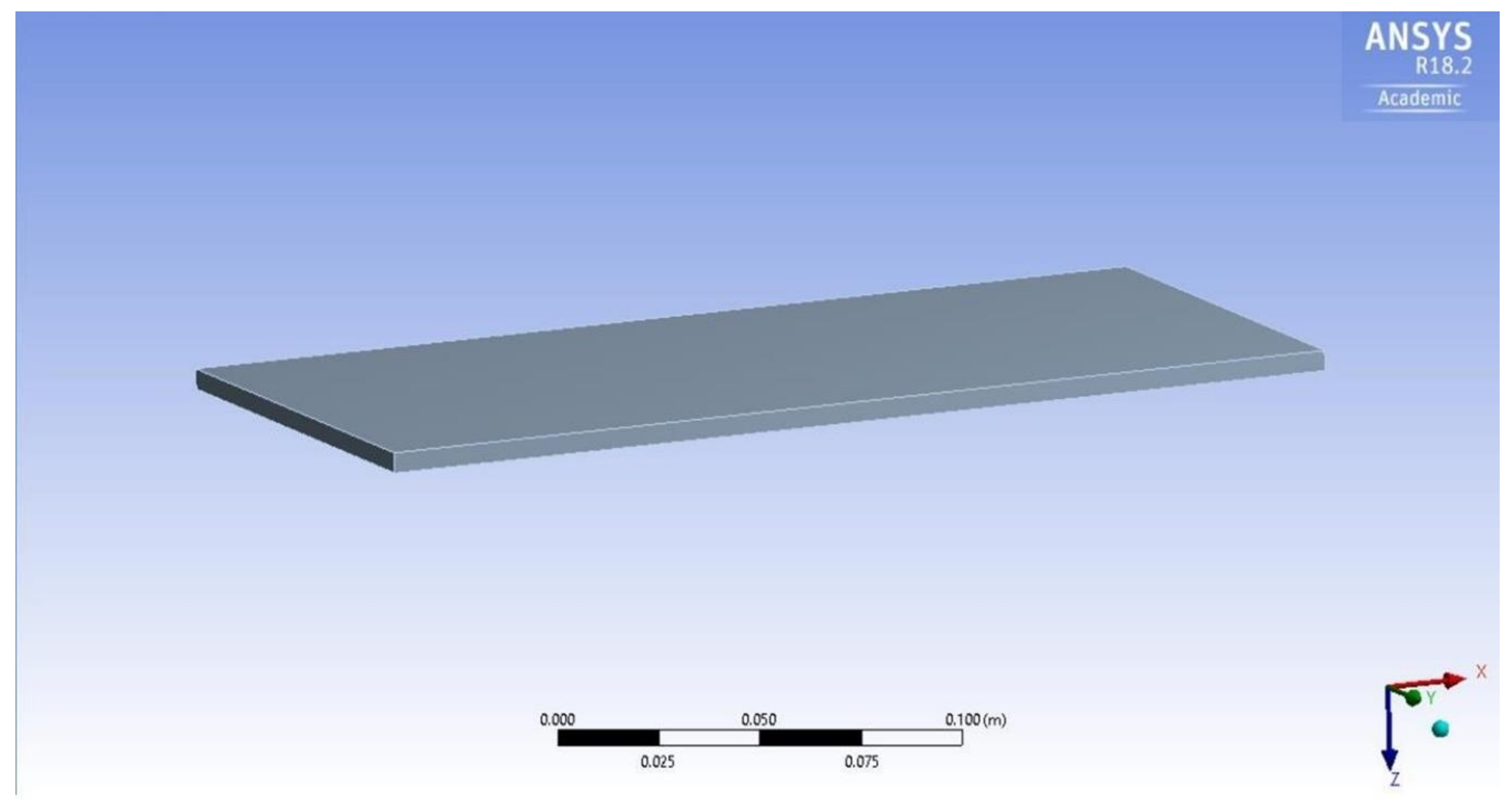
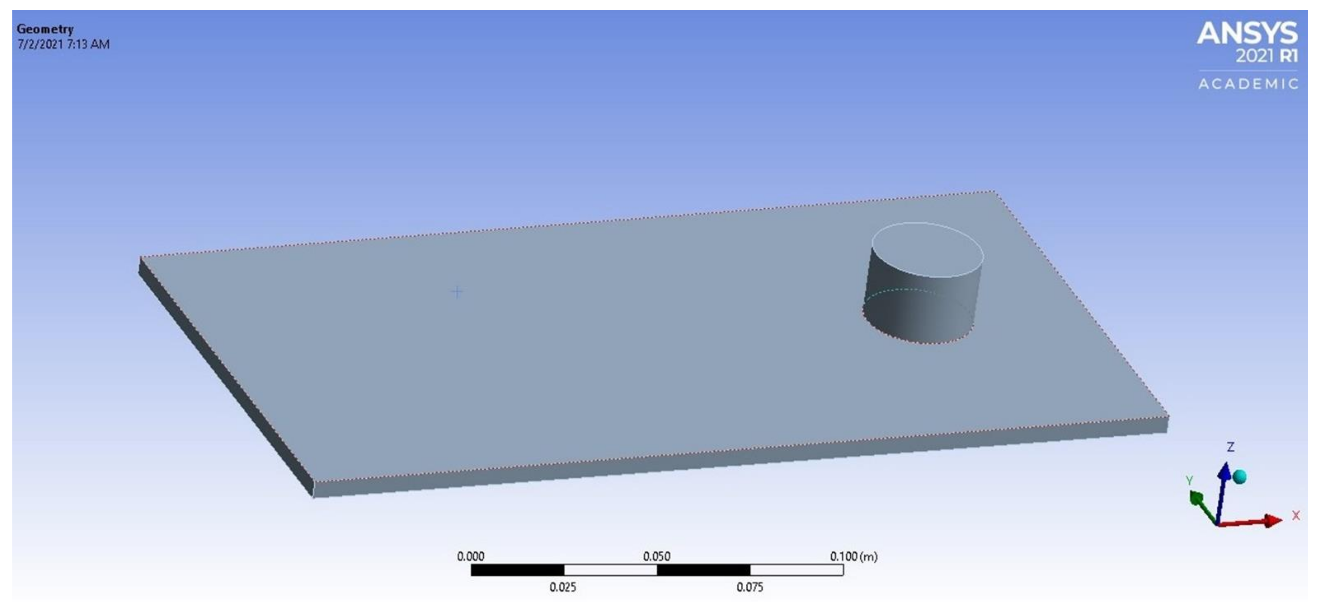
2.1. Materials
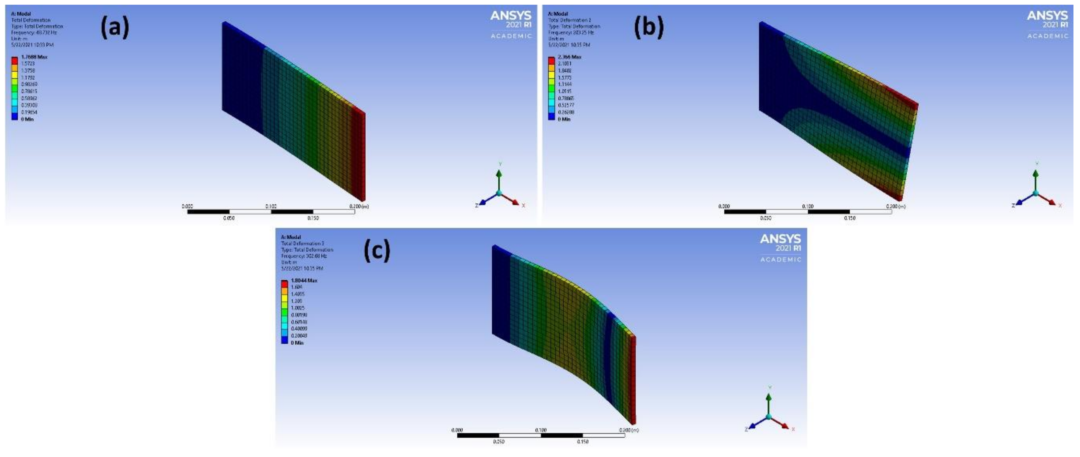
2.2. Modal Analysis
Kirchhoff Thin Plate Model
2.3. Data Processing
2.3.1. Deep Learning Approach
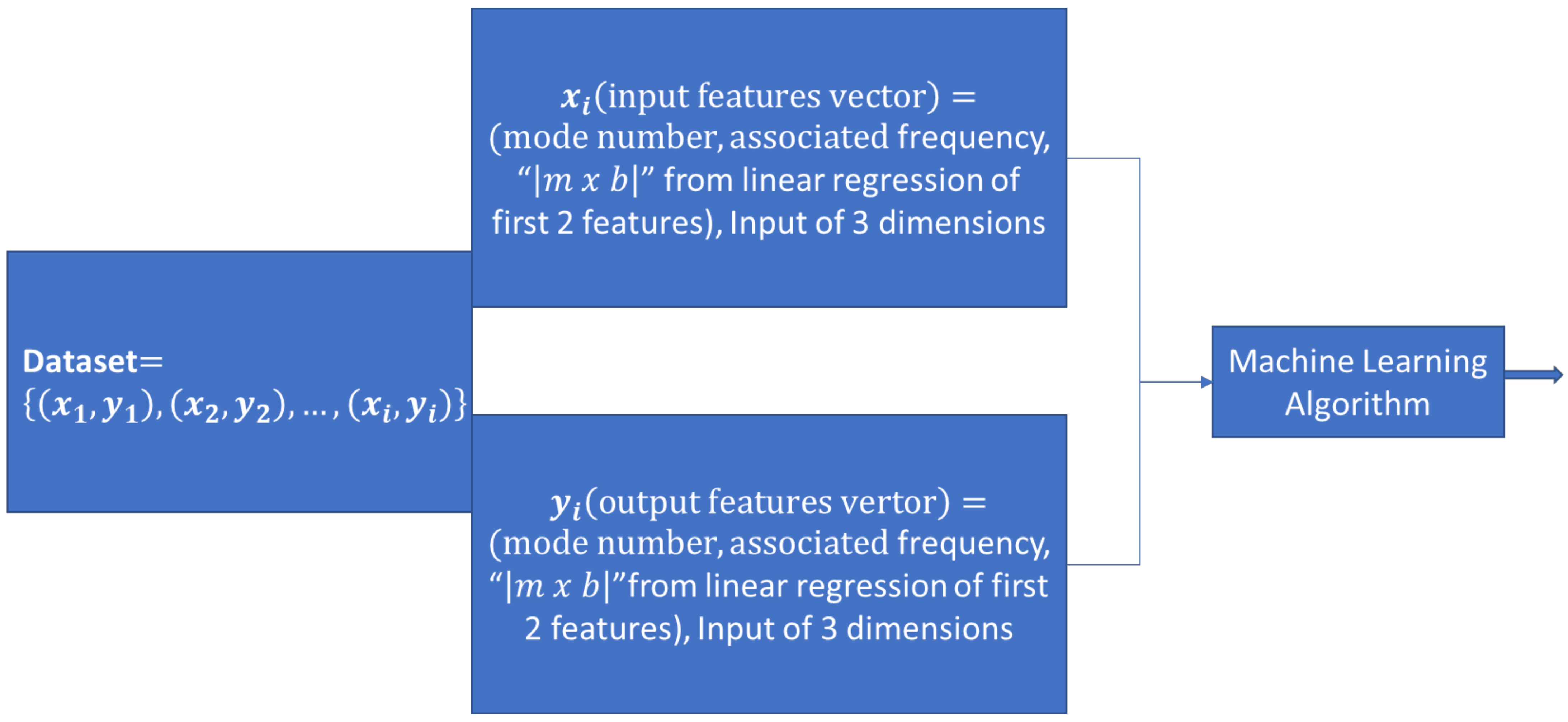
2.3.2. Machine Learning Approach
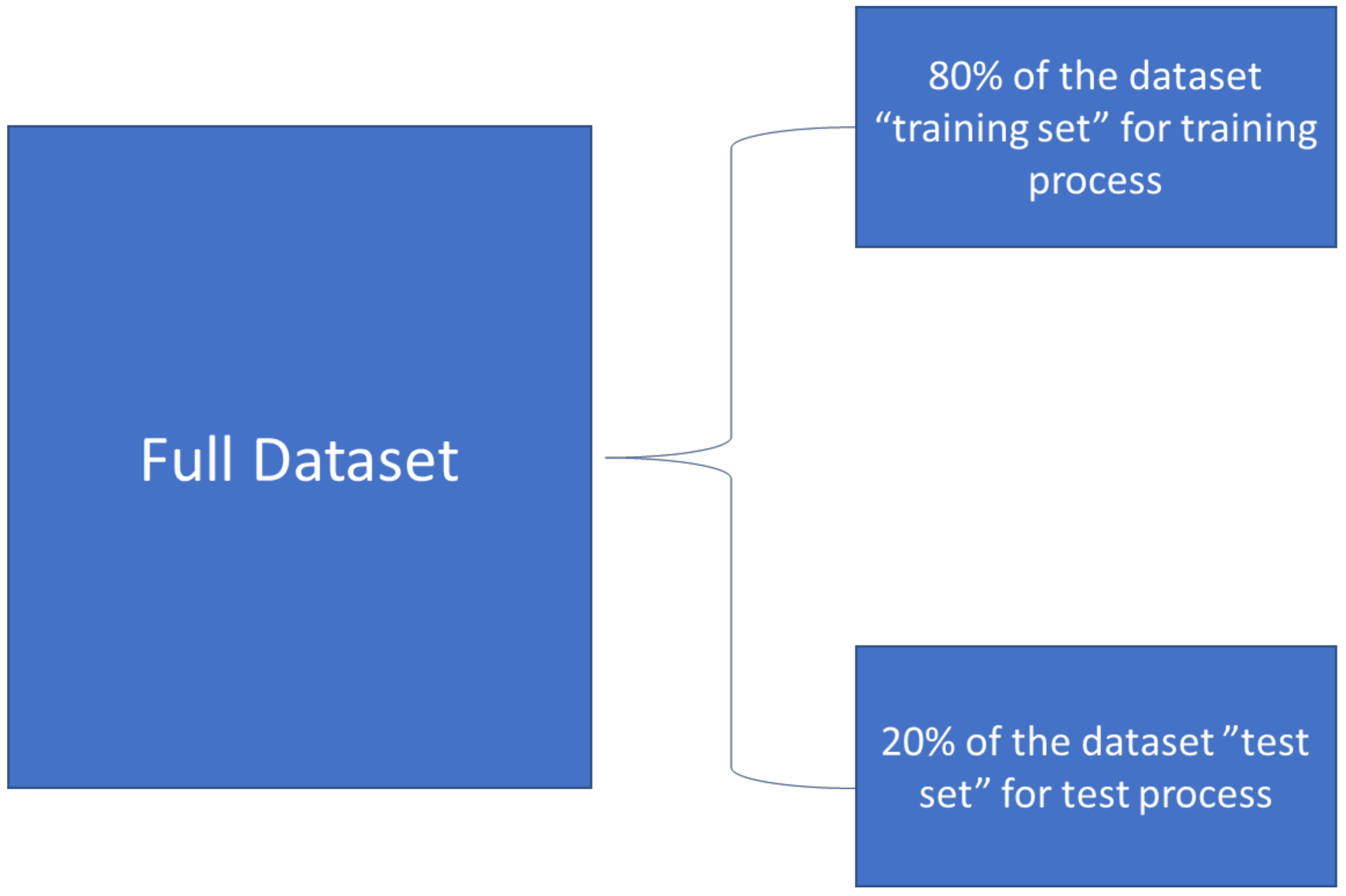
2.3.3. Model Evaluation
2.3.4. Data Processing and Analysis
3. Results and Discussions
3.1. Isotropic Materials
3.2. Orthotropic Materials
4. Conclusions
- The study demonstrated the ability to classify engineering materials, including isotropic and orthotropic materials, by applying ML algorithms on the modal analysis results. The proposed ML approaches could reach an accuracy of 100% when interrelations were created between the inputs to the ML algorithms (combined linear regression approach in this study).
- The Keras model was not suitable for this study as it showed 50% accuracy when compared to the ML approaches. The study validates the classification applicability based on the resonance frequency information, which may broaden the horizon of further applications such as a device that can classify the materials based on their modal analysis.
- The study showed a novel method of using the extracted data from modal analysis to accurately classify and identify the engineering materials as well as validate the efficiency of using induced interrelations between the mode number and its corresponding resonance frequency to increase the accuracy of the proposed machine learning methods.
- The study validated the classification applicability based on the resonance frequency information, which may broaden the horizon of further applications such as a device that can classify the materials based on their modal analysis. A further study could include other modal analysis parameters, such as damping ratios using experimental data as it will be by default assumed to be zero in ANSYS.
- Potential future studies can study other DL approaches and the deployment of neural networks that could achieve promising classification studies. Further extensions and relations can be established for detailed material properties identification through deploying the concept of ML and DL into the field of mechanical engineering, which would further confirm the modern concept of science integration.
- The results of this study can boost non-destructive materials characterizations and analysis methods in general, not just the explored modal analysis example, as ML and DL deal mainly with data regardless of the acquiring method.
Author Contributions
Funding
Institutional Review Board Statement
Informed Consent Statement
Data Availability Statement
Conflicts of Interest
References
- Noman, M.T.; Amor, N.; Petru, M. Synthesis and applications of ZnO nanostructures (ZONSs): A review. Crit. Rev. Solid State Mater. Sci. 2021, 1–43. [Google Scholar] [CrossRef]
- Schmitz, T.L.; Smith, K.S. Machining Dynamics; Springer: Berlin/Heidelberg, Germany, 2014. [Google Scholar]
- Van Woensel, G.; Verdonck, E.; De Baerdemaeker, J. Measuring the mechanical properties of apple tissue using modal analysis. J. Food Process Eng. 1988, 10, 151–163. [Google Scholar] [CrossRef]
- Amor, N.; Rasool, G.; Bouaynaya, N.C.; Shterenberg, R. Constrained particle filtering for movement identification in forearm prosthesis. Signal Process. 2019, 161, 25–35. [Google Scholar] [CrossRef]
- Meddeb, A.; Amor, N.; Abbes, M.; Chebbi, S. A novel approach based on crow search algorithm for solving reactive power dispatch problem. Energies 2018, 11, 3321. [Google Scholar] [CrossRef] [Green Version]
- Noman, M.T.; Petrů, M. Functional properties of sonochemically synthesized zinc oxide nanoparticles and cotton composites. Nanomaterials 2020, 10, 1661. [Google Scholar] [CrossRef] [PubMed]
- Noman, M.T.; Petru, M.; Amor, N.; Louda, P. Thermophysiological comfort of zinc oxide nanoparticles coated woven fabrics. Sci. Rep. 2020, 10, 21080. [Google Scholar]
- Noman, M.T.; Petru, M.; Militký, J.; Azeem, M.; Ashraf, M.A. One-Pot Sonochemical Synthesis of ZnO Nanoparticles for Photocatalytic Applications, Modelling and Optimization. Materials 2020, 13, 14. [Google Scholar] [CrossRef] [PubMed] [Green Version]
- Islam, K.T.; Wijewickrema, S.; O’Leary, S. A deep learning based framework for the registration of three dimensional multi-modal medical images of the head. Sci. Rep. 2021, 11, 1860. [Google Scholar] [CrossRef]
- Zhao, Y.; Chang, C.; Hannum, M.; Lee, J.; Shen, R. Bayesian network-driven clustering analysis with feature selection for high-dimensional multi-modal molecular data. Sci. Rep. 2021, 11, 5146. [Google Scholar]
- Noman, M.T.; Militky, J.; Wiener, J.; Saskova, J.; Ashraf, M.A.; Jamshaid, H.; Azeem, M. Sonochemical synthesis of highly crystalline photocatalyst for industrial applications. Ultrasonics 2018, 83, 203–213. [Google Scholar] [CrossRef]
- Noman, M.T.; Petru, M. Effect of Sonication and Nano TiO2 on Thermophysiological Comfort Properties of Woven Fabrics. ACS Omega 2020, 5, 11481–11490. [Google Scholar] [CrossRef] [PubMed]
- Noman, M.T.; Petru, M.; Amor, N.; Yang, T.; Mansoor, T. Thermophysiological comfort of sonochemically synthesized nano TiO2 coated woven fabrics. Sci. Rep. 2020, 10, 17204. [Google Scholar] [CrossRef] [PubMed]
- Noman, M.T.; Wiener, J.; Saskova, J.; Ashraf, M.A.; Vikova, M.; Jamshaid, H.; Kejzlar, P. In-situ development of highly photocatalytic multifunctional nanocomposites by ultrasonic acoustic method. Ultrason. Sonochem. 2018, 40, 41–56. [Google Scholar] [CrossRef] [PubMed]
- Mahmood, A.; Noman, M.T.; Pechočiaková, M.; Amor, N.; Petrů, M.; Abdelkader, M.; Militký, J.; Sozcu, S.; Hassan, S.Z.U. Geopolymers and Fiber-Reinforced Concrete Composites in Civil Engineering. Polymers 2021, 13, 2099. [Google Scholar] [CrossRef] [PubMed]
- Anastasopoulos, D.; De Roeck, G.; Reynders, E.P. One-year operational modal analysis of a steel bridge from high-resolution macrostrain monitoring: Influence of temperature vs. retrofitting. Mech. Syst. Signal Process. 2021, 161, 107951. [Google Scholar] [CrossRef]
- Carpine, R.; Ientile, S.; Vacca, N.; Boscato, G.; Rospars, C.; Cecchi, A.; Argoul, P. Modal identification in the case of complex modes–Use of the wavelet analysis applied to the after-shock responses of a masonry wall during shear compression tests. Mech. Syst. Signal Process. 2021, 160, 107753. [Google Scholar] [CrossRef]
- Fang, C.; Zhang, Y. An improved hybrid FE-SEA model using modal analysis for the mid-frequency vibro-acoustic problems. Mech. Syst. Signal Process. 2021, 161, 107957. [Google Scholar] [CrossRef]
- Abo-Elkhier, M.; Hamada, A.; El-Deen, A.B. Prediction of fatigue life of glass fiber reinforced polyester composites using modal testing. Int. J. Fatigue 2014, 69, 28–35. [Google Scholar] [CrossRef]
- El-Labban, H.F.; AbdelAziz, M.; Yakout, M.; Elkhatib, A. Prediction of mechanical properties of nano-composites using vibration modal analysis: Application to aluminum piston alloys. Mater. Perform. Charact. 2013, 2, 454–467. [Google Scholar] [CrossRef]
- Yakout, M.; Elkhatib, A.; Nassef, M. Rolling element bearings absolute life prediction using modal analysis. J. Mech. Sci. Technol. 2018, 32, 91–99. [Google Scholar] [CrossRef]
- Chang, K.-C.; Kim, C.-W. Modal-parameter identification and vibration-based damage detection of a damaged steel truss bridge. Eng. Struct. 2016, 122, 156–173. [Google Scholar] [CrossRef]
- Guan, C.; Zhang, H.; Wang, X.; Miao, H.; Zhou, L.; Liu, F. Experimental and theoretical modal analysis of full-sized wood composite panels supported on four nodes. Materials 2017, 10, 683. [Google Scholar] [CrossRef] [PubMed] [Green Version]
- Noman, M.T.; Amor, N.; Petru, M.; Mahmood, A.; Kejzlar, P. Photocatalytic Behaviour of Zinc Oxide Nanostructures on Surface Activation of Polymeric Fibres. Polymers 2021, 13, 1227. [Google Scholar] [CrossRef] [PubMed]
- LeCun, Y.; Bengio, Y.; Hinton, G. Deep learning. Nature 2015, 521, 436–444. [Google Scholar] [CrossRef] [PubMed]
- Noman, M.T.; Petru, M.; Louda, P. Woven textiles coated with zinc oxide nanoparticles and their thermophysiological comfort properties. J. Nat. Fibers 2021, 1–13. [Google Scholar] [CrossRef]
- Sathya, R.; Abraham, A. Comparison of supervised and unsupervised learning algorithms for pattern classification. Int. J. Adv. Res. Artif. Intell. 2013, 2, 34–38. [Google Scholar] [CrossRef] [Green Version]
- Li, Y.; Anderson-Sprecher, R. Facies identification from well logs: A comparison of discriminant analysis and naïve Bayes classifier. J. Pet. Sci. Eng. 2006, 53, 149–157. [Google Scholar] [CrossRef]
- Noman, M.T.; Ashraf, M.A.; Ali, A. Synthesis and applications of nano-TiO2: A review. Environ. Sci. Pollut. Res. 2019, 26, 3262–3291. [Google Scholar] [CrossRef]
- Noman, M.T.; Ashraf, M.A.; Jamshaid, H.; Ali, A. A novel green stabilization of TiO2 nanoparticles onto cotton. Fibers Polym. 2018, 19, 2268–2277. [Google Scholar] [CrossRef]
- Isobe, T.; Feigelson, E.D.; Akritas, M.G.; Babu, G.J. Linear regression in astronomy. Astrophys. J. 1990, 364, 104–113. [Google Scholar] [CrossRef]
- Amor, N.; Noman, M.T.; Petru, M. Prediction of functional properties of nano TiO2 coated cotton composites by artificial neural network. Sci. Rep. 2021, 11, 12235. [Google Scholar] [CrossRef]
- Amor, N.; Noman, M.T.; Petru, M.; Mahmood, A.; Ismail, A. Neural network-crow search model for the prediction of functional properties of nano TiO2 coated cotton composites. Sci. Rep. 2021, 11, 13649. [Google Scholar]


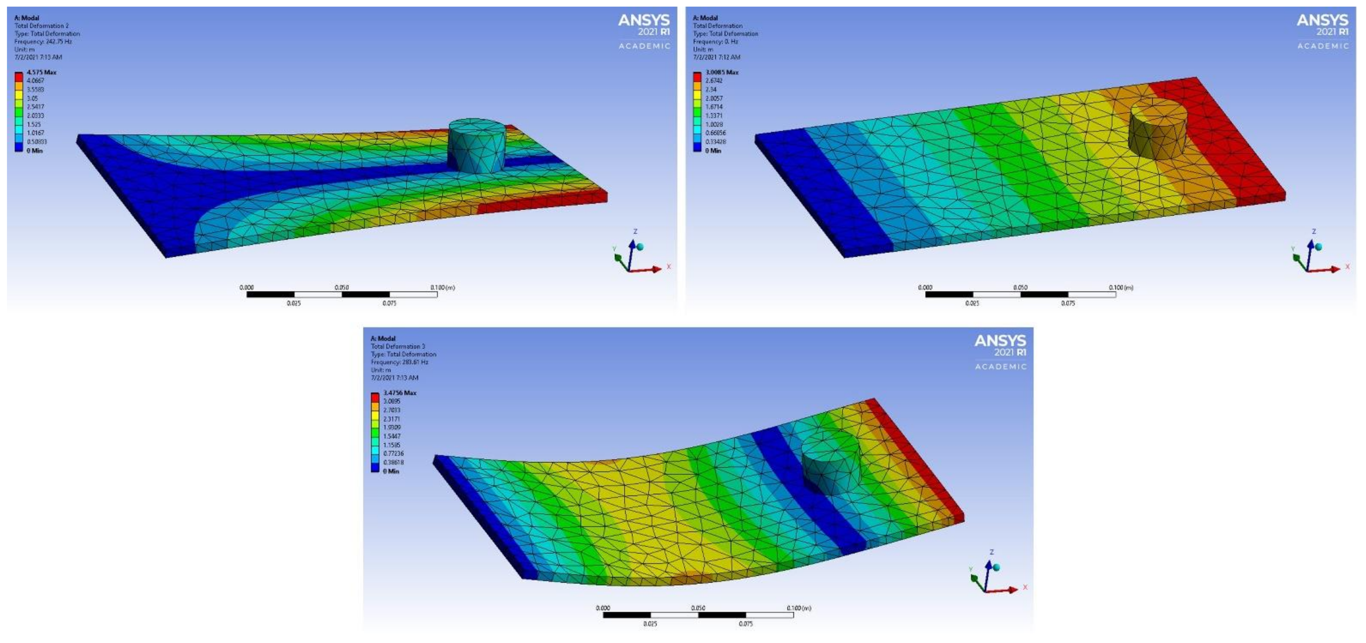
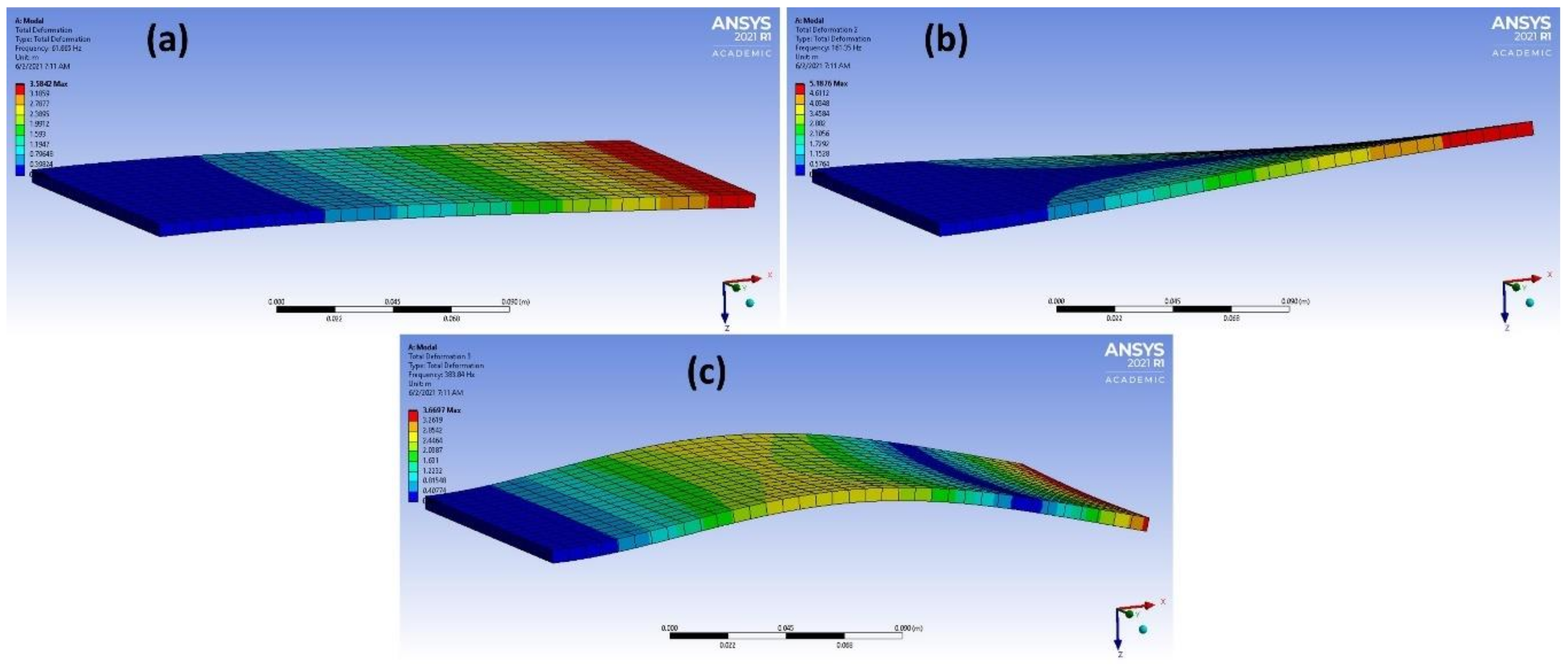
| Mode Number | Frequency for the Studied Materials [Hz] | |||
|---|---|---|---|---|
| Stainless Steel | Magnesium | Epoxy Carbon Woven (230 GPa) Wet | Epoxy E-Glass UD | |
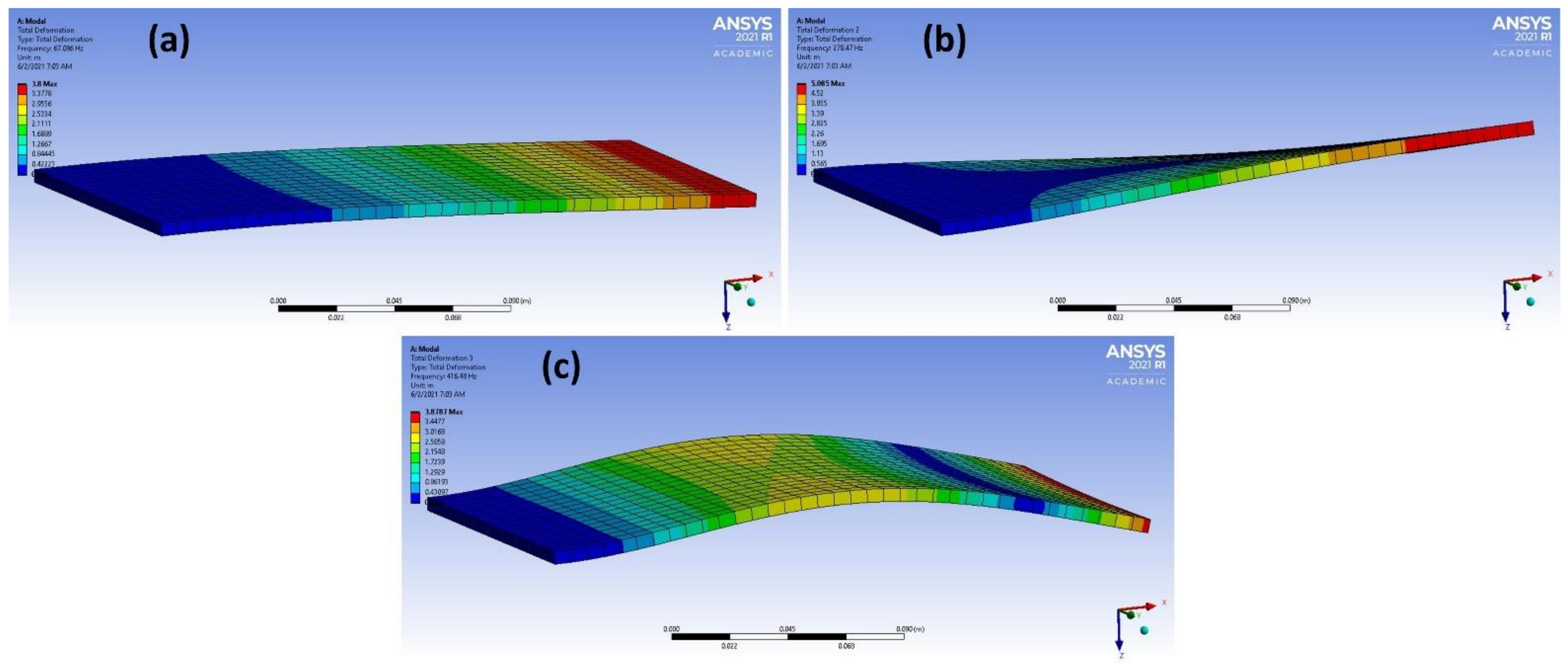
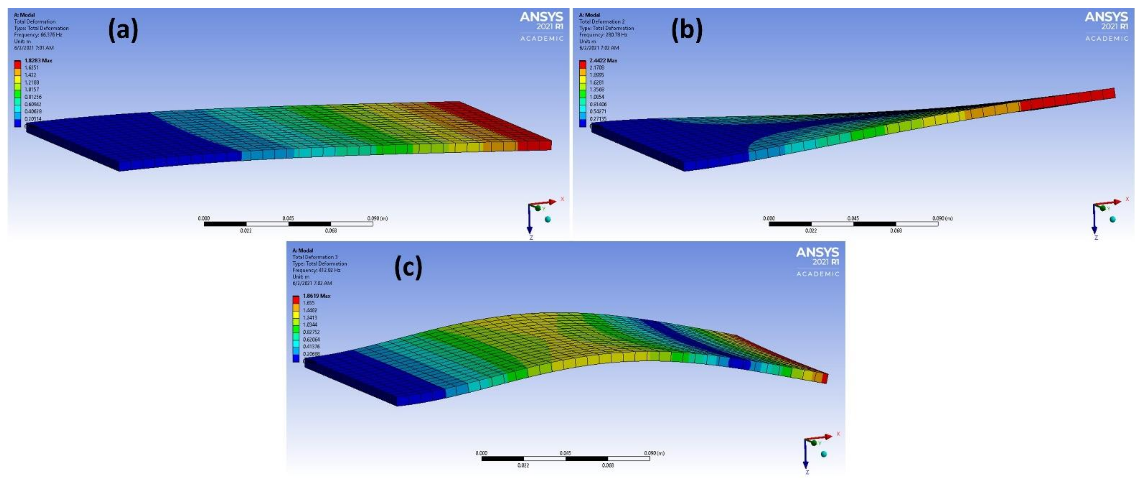
| 1 | 66.376 | 67.086 | 82.419 | 61.665 |
| 2 | 280.78 | 278.47 | 169.44 | 161.35 |
| 3 | 412.82 | 416.48 | 511.09 | 383.84 |
| Accuracy | Logistic Regression | Decision Tree | K-Nearest Neighbors | Linear Discriminant | Naive Bayes | Support Vector Machine |
|---|---|---|---|---|---|---|
| Training set | 0.55 | 1.00 | 0.51 | 0.56 | 0.51 | 1.00 |
| Test set | 0.50 | 0.50 | 0.50 | 0.50 | 0.50 | 0.50 |
| Accuracy | Logistic Regression | Decision Tree | K-Nearest Neighbors | Linear Discriminant | Naive Bayes | Support Vector Machine |
|---|---|---|---|---|---|---|
| Training set | 1.00 | 1.00 | 1.00 | 0.56 | 1.00 | 1.00 |
| Test set | 0.88 | 1.00 | 1.00 | 0.50 | 1.00 | 0.50 |
| Accuracy | Logistic Regression | Decision Tree | K-Nearest Neighbors | Linear Discriminant | Naive Bayes | Support Vector Machine |
|---|---|---|---|---|---|---|
| Training set | 0.88 | 1.00 | 1.00 | 0.96 | 1.00 | 1.00 |
| Test set | 0.68 | 1.00 | 1.00 | 1.00 | 1.00 | 0.50 |
| Accuracy | Logistic Regression | Decision Tree | K-Nearest Neighbors | Linear Discriminant | Naive Bayes | Support Vector Machine |
|---|---|---|---|---|---|---|
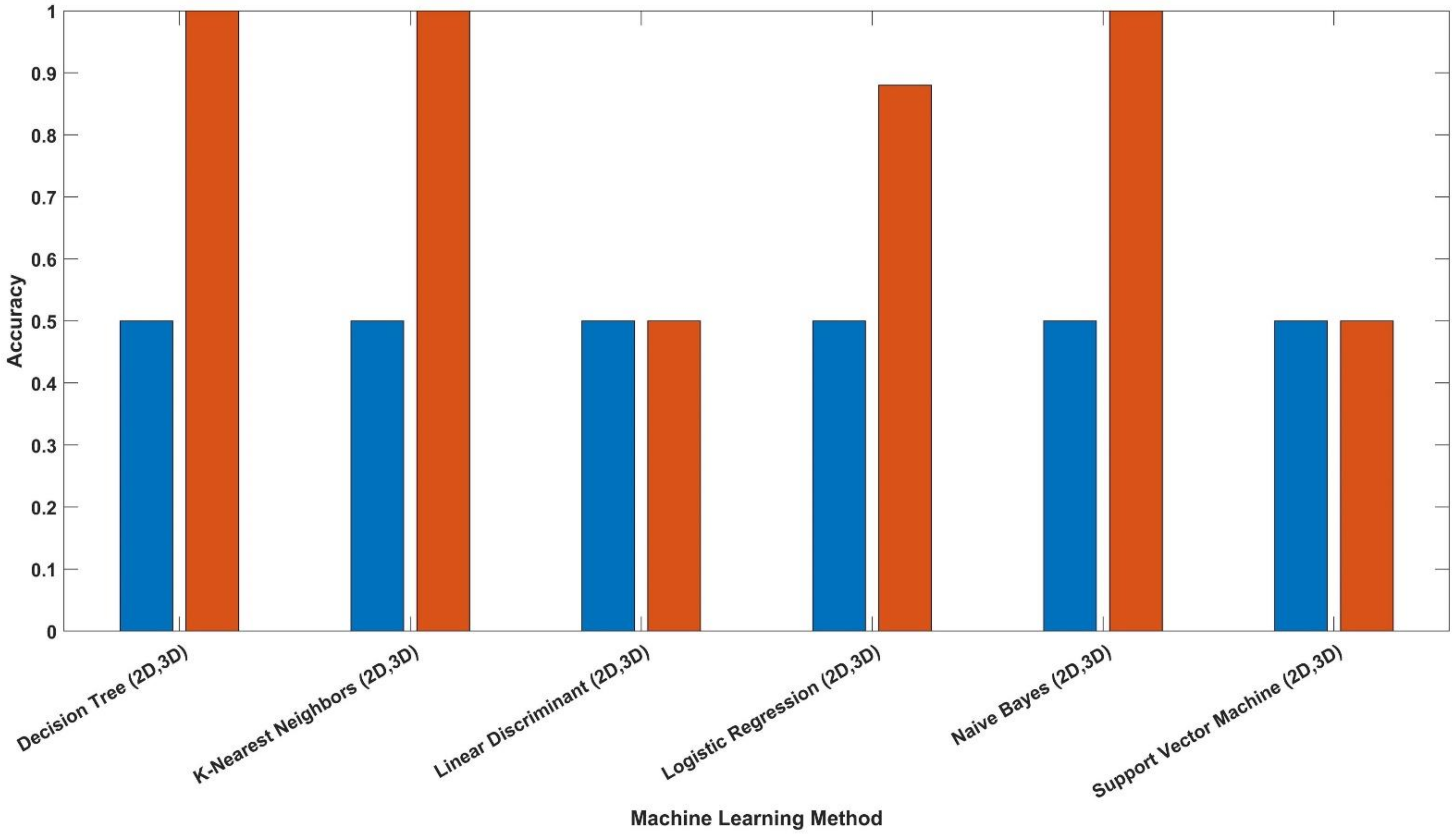
| Isotropic | 0.88 | 1.00 | 1.00 | 0.50 | 1.00 | 0.50 |
| Orthotropic | 0.68 | 1.00 | 1.00 | 1.00 | 1.00 | 0.50 |
Publisher’s Note: MDPI stays neutral with regard to jurisdictional claims in published maps and institutional affiliations. |
© 2021 by the authors. Licensee MDPI, Basel, Switzerland. This article is an open access article distributed under the terms and conditions of the Creative Commons Attribution (CC BY) license (https://creativecommons.org/licenses/by/4.0/).
Share and Cite
Abdelkader, M.; Noman, M.T.; Amor, N.; Petru, M.; Mahmood, A. Combined Use of Modal Analysis and Machine Learning for Materials Classification. Materials 2021, 14, 4270. https://doi.org/10.3390/ma14154270
Abdelkader M, Noman MT, Amor N, Petru M, Mahmood A. Combined Use of Modal Analysis and Machine Learning for Materials Classification. Materials. 2021; 14(15):4270. https://doi.org/10.3390/ma14154270
Chicago/Turabian StyleAbdelkader, Mohamed, Muhammad Tayyab Noman, Nesrine Amor, Michal Petru, and Aamir Mahmood. 2021. "Combined Use of Modal Analysis and Machine Learning for Materials Classification" Materials 14, no. 15: 4270. https://doi.org/10.3390/ma14154270
APA StyleAbdelkader, M., Noman, M. T., Amor, N., Petru, M., & Mahmood, A. (2021). Combined Use of Modal Analysis and Machine Learning for Materials Classification. Materials, 14(15), 4270. https://doi.org/10.3390/ma14154270