
Material Properties of HY 80 Steel after 55 Years of Operation for FEM Applications


Abstract
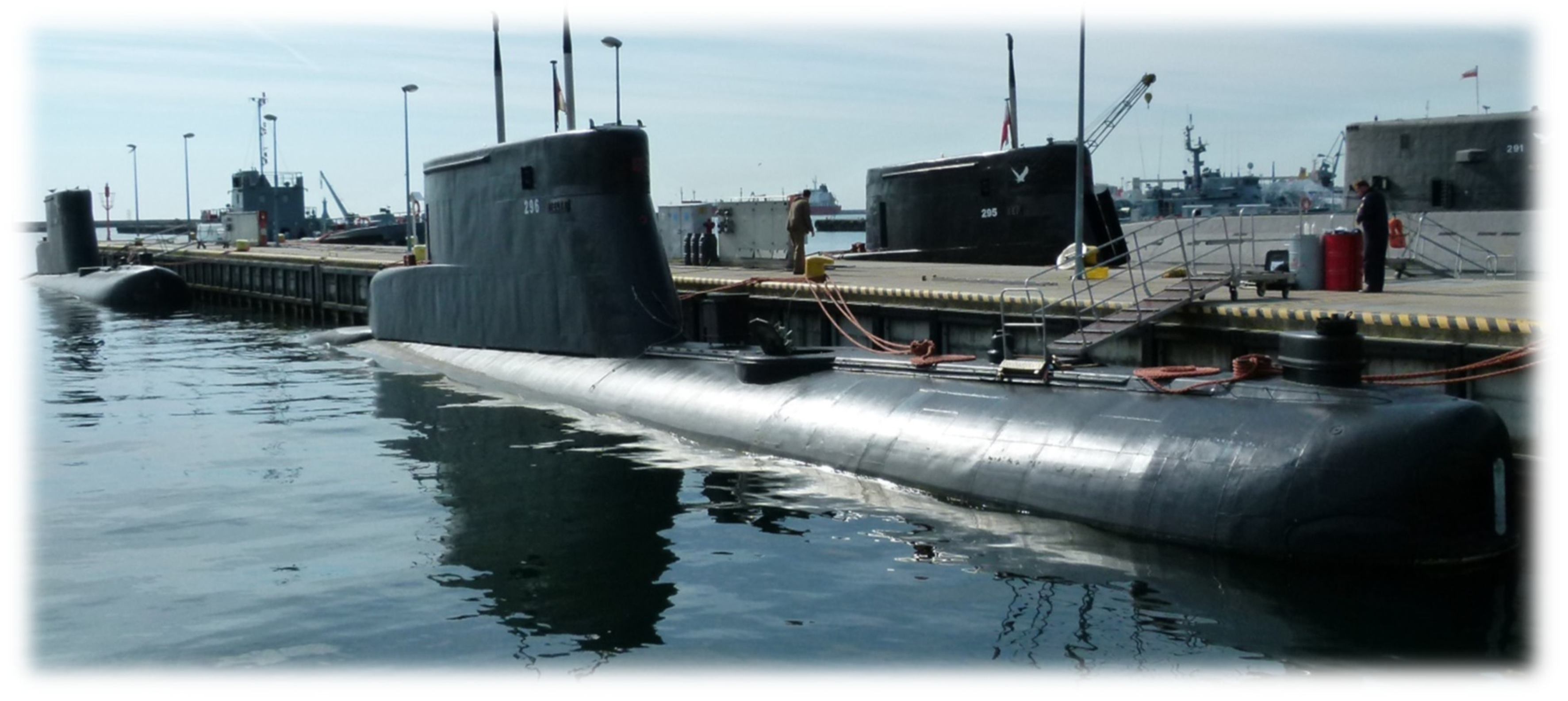
:1. Introduction
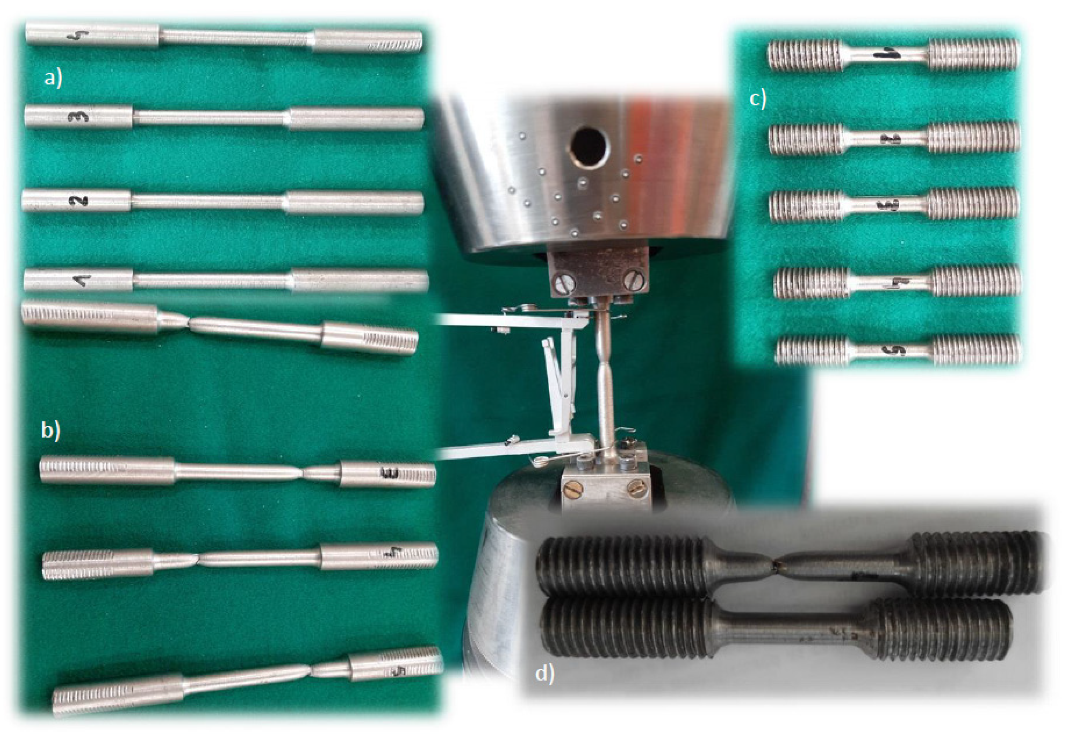
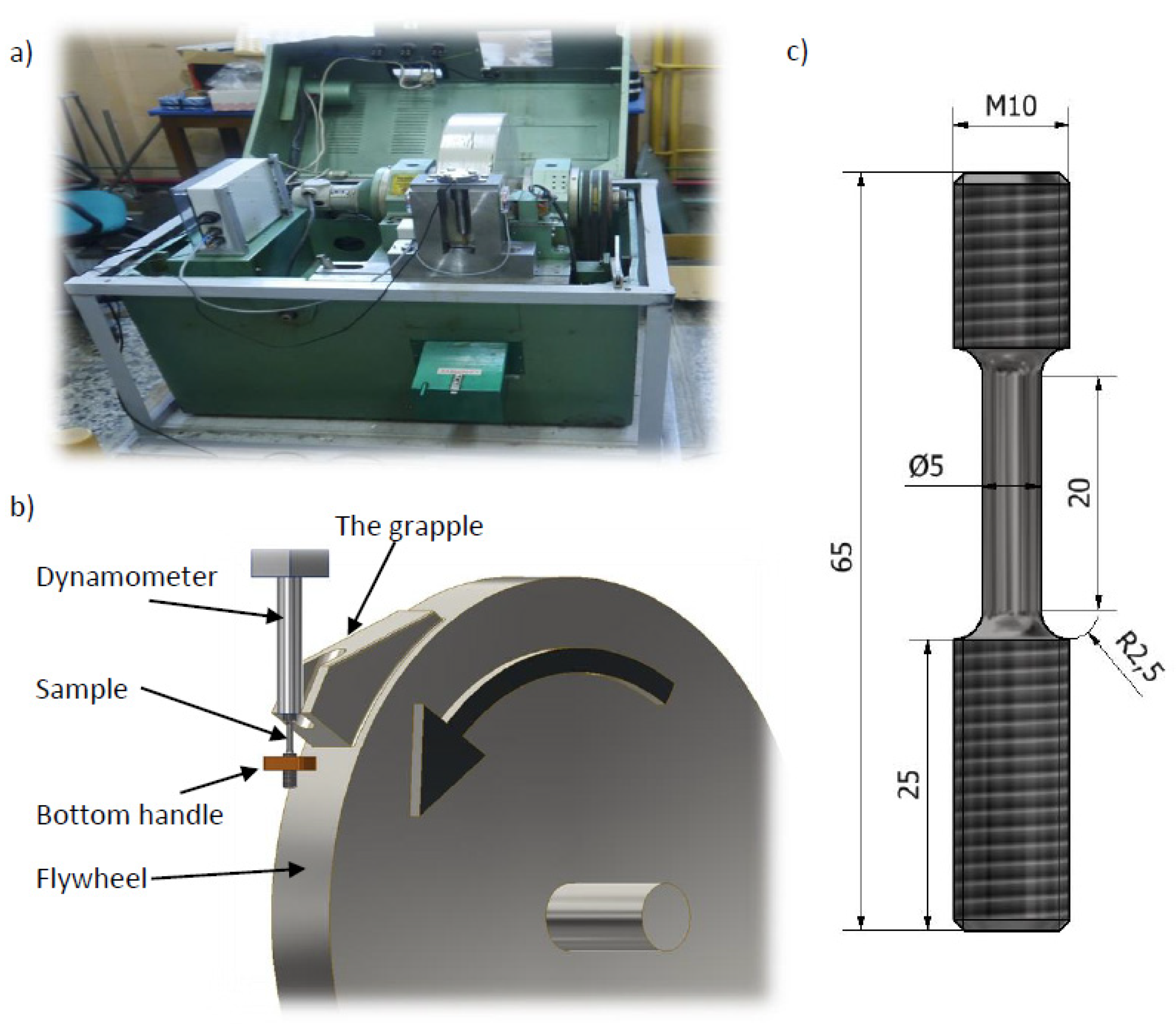
2. Materials and Methods
3. Results
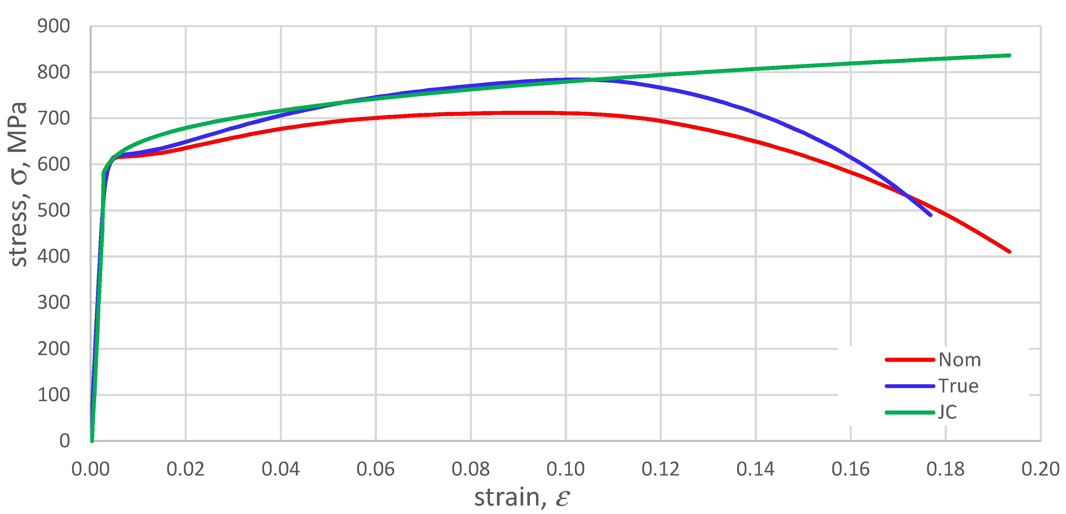
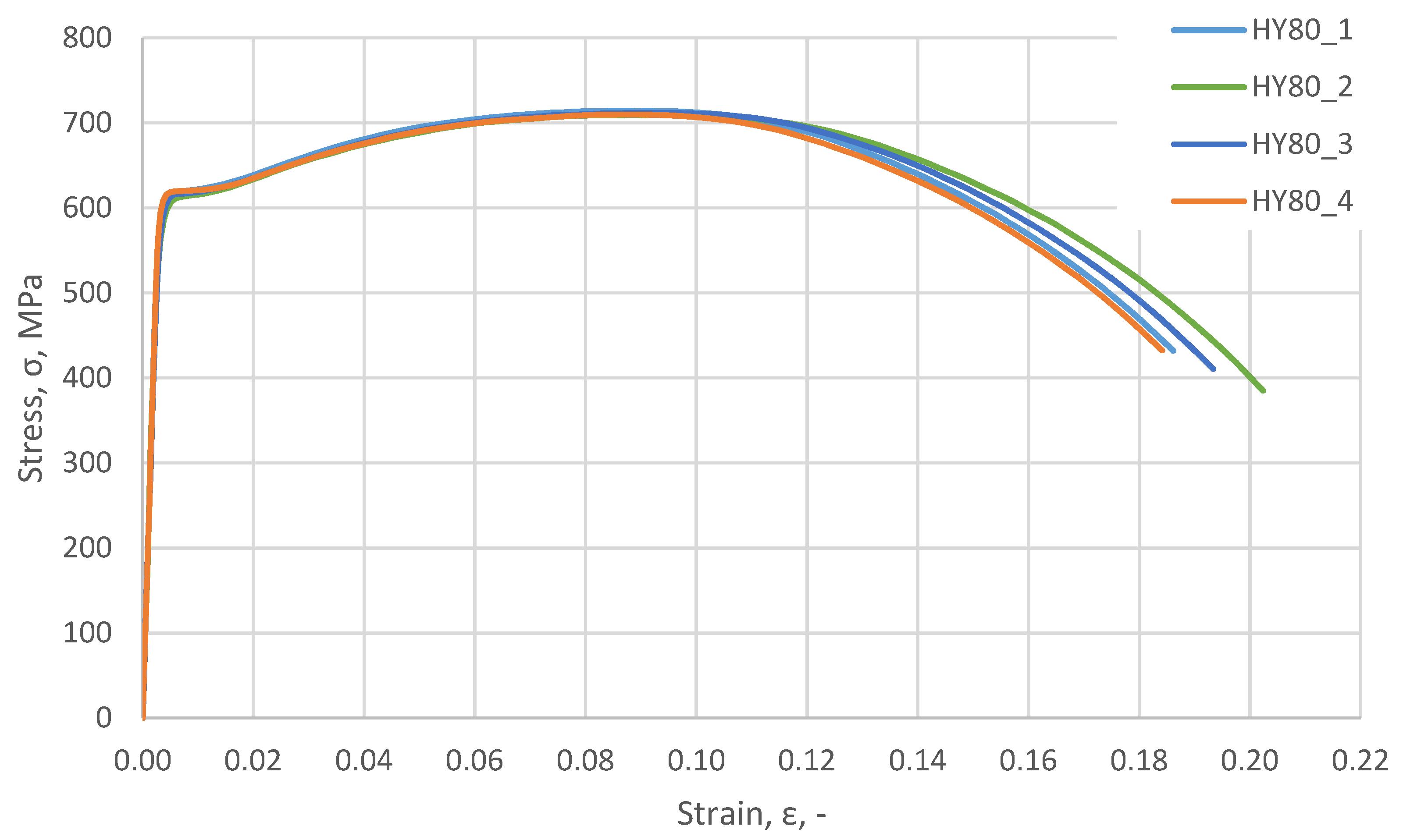
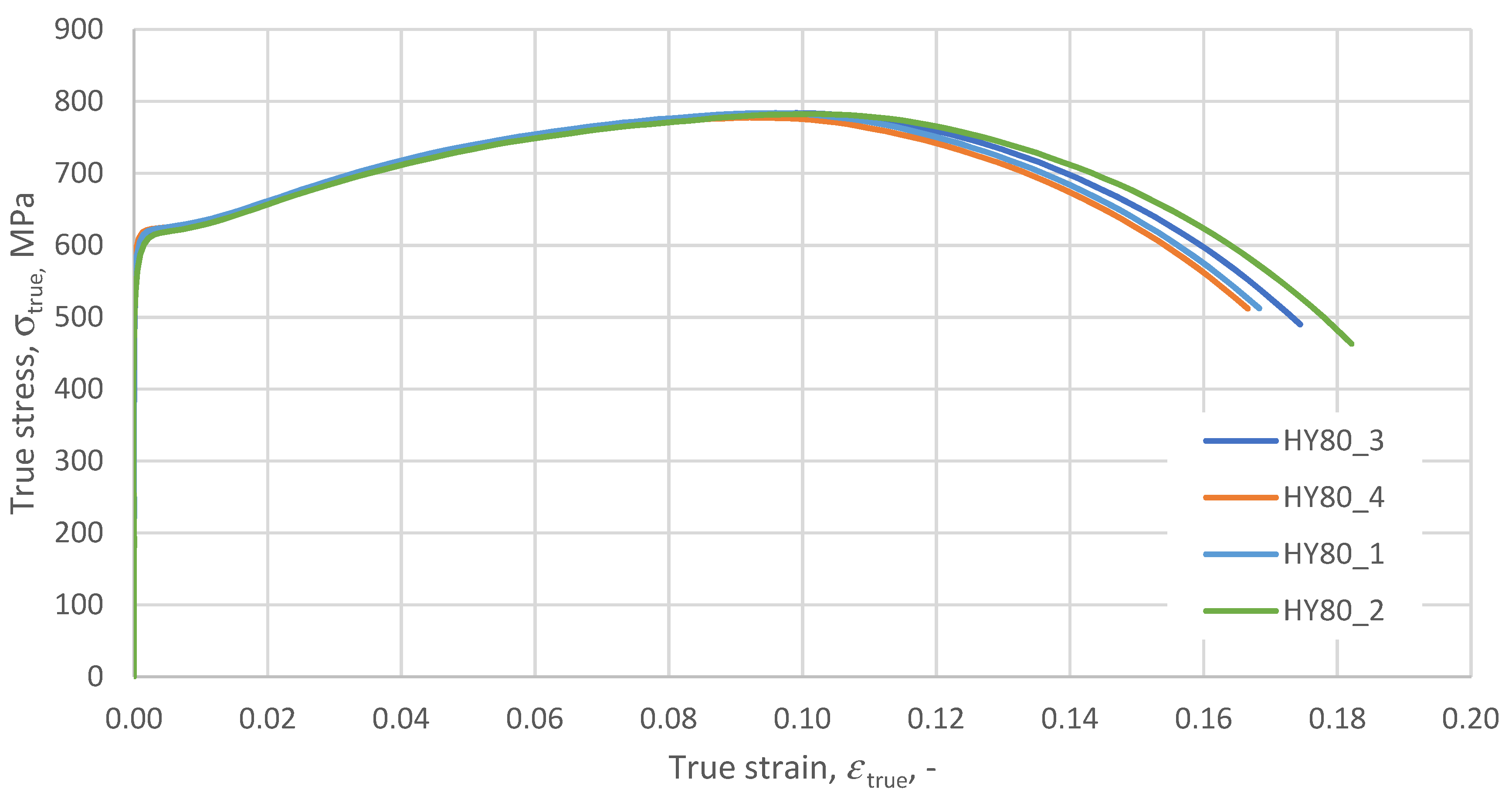
3.1. Uniaxial Static Tensile Test
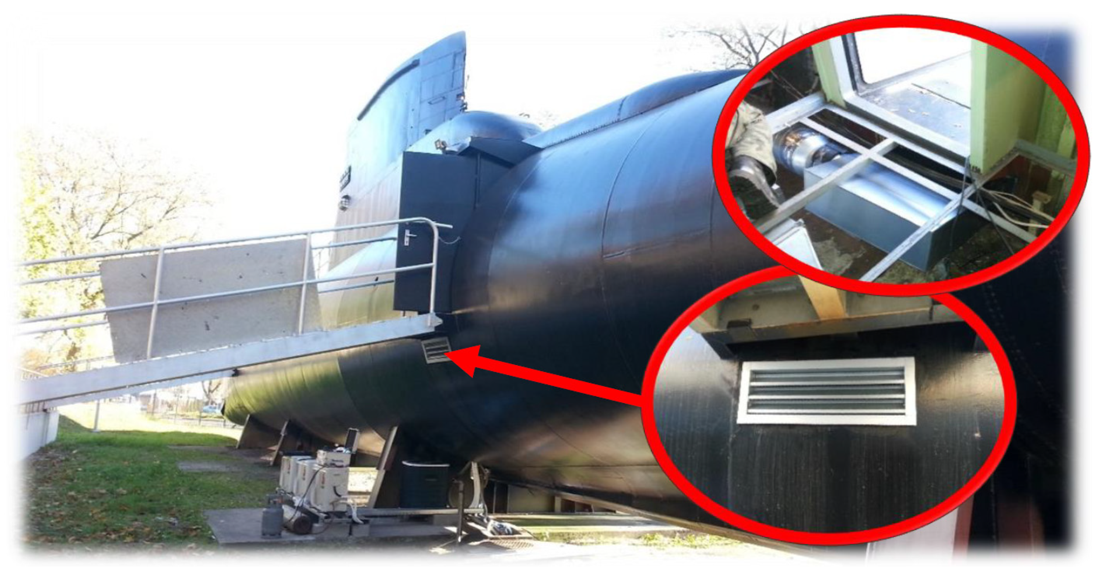
3.2. The Study of Dynamic Mechanical Properties Using a Rotary Hammer
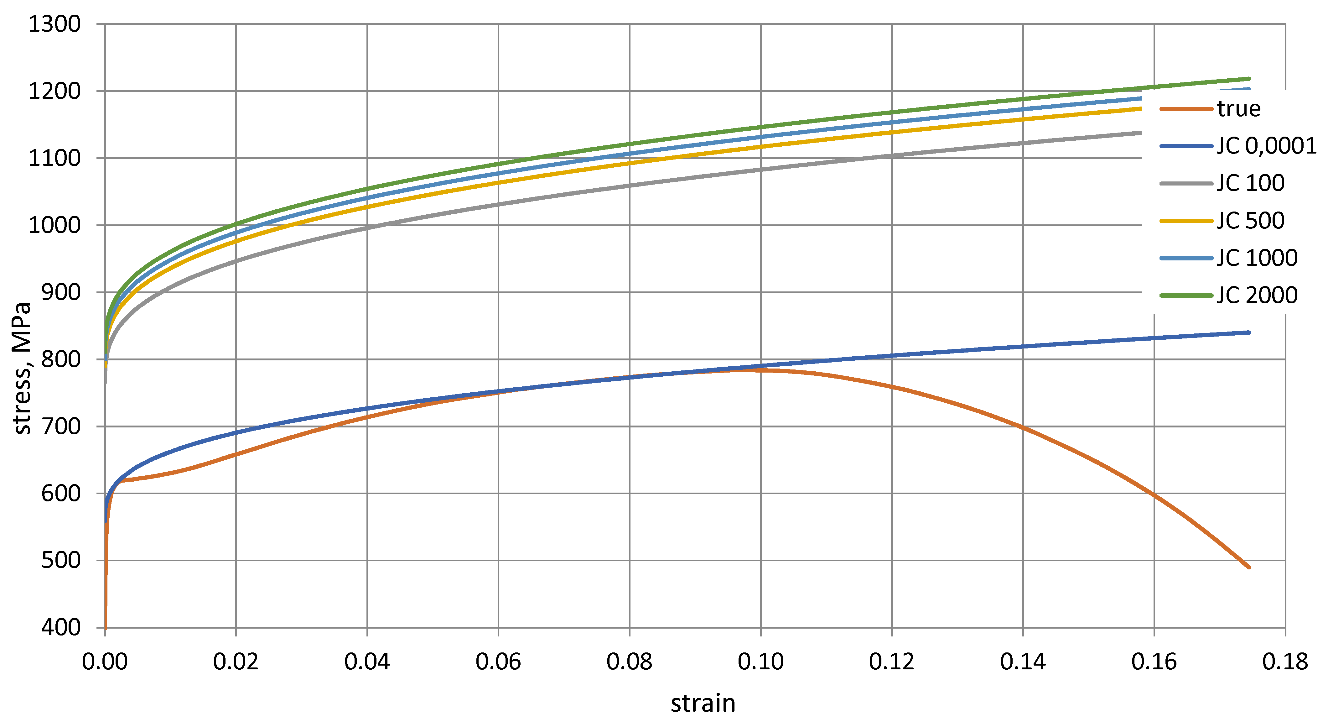
3.3. HY 80 True Characteristics
- A–elastic range of the material (it is often simplified in form A = Re);
- B–hardening parameter;
- n–hardening exponent;
- C–strain rate coefficient;
- –true plastic strain;
- –strain rate;
- –quasi-static strain rate (0.0001 s−1);
- θ–current material temperature;
- θ0–ambient temperature;
- θtmelt–melting temperature;
- m–thermal softening exponent.
- A = 559 MPa;
- B = 518 MPa;
- n = 0.379.
- Ambient temperature θ0 = 293.15 K;
- Melting temperature θtop = 1733 ~ 1793;
- Thermal coefficient m = 0.75 ÷ 1.15.
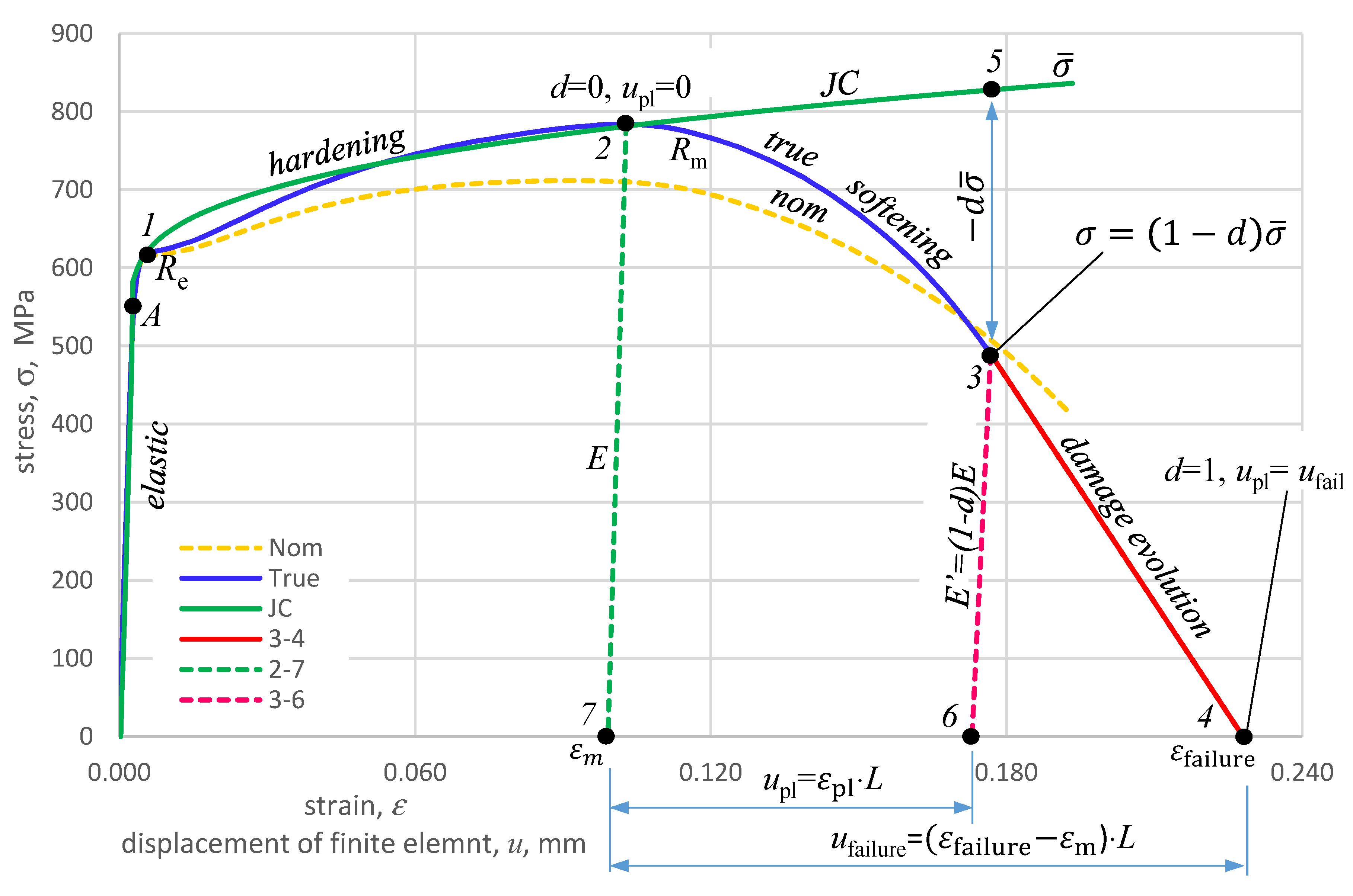
3.4. HY 80 Steel Failure at Uniaxial Tension
4. Discussion
5. Conclusions
Author Contributions
Funding
Institutional Review Board Statement
Informed Consent Statement
Data Availability Statement
Conflicts of Interest
References
- Holmquist, T.J. Strenght and Fracture Characteristics of HY-80, HY-100, and HY-130 Steels Subjected to Various Strains, Strain Rates Temperatures, Adn Pressures; Nacal Surface Warfare Center, NSWC: Dahlgren, VA, USA, 1987. [Google Scholar]
- Lee, J.; Lee, K.; Lee, S.; Kwon, O.M.; Kang, W.-K.; Lim, J.-I.; Lee, H.-K.; Kim, S.-M.; Kwon, D. Application of Macro-Instrumented Indentation Test for Superficial Residual Stress and Mechanical Properties Measurement for HY Steel Welded T-Joints. Materials 2021, 14, 2061. [Google Scholar] [CrossRef] [PubMed]
- Kut, S. State of Stress Identification in Numerical Modeling of 3D Issues. Arch. Metall. Mater. 2009, 54, 628–632. [Google Scholar]
- Konieczny, J. Materiały Konstrukcyjne Okrętów (Ship Construction Materials). Kwartalnik Bellona 2009, 658, 153–159. [Google Scholar]
- Okręty Podwodne Typu Kobben-Defence24. Available online: https://www.defence24.pl/okrety-podwodne-typu-kobben (accessed on 8 November 2020).
- Rajendran, A.M.; Last, H.R.; Garrett, R.K. Plastic Flow and Failure in HY100, HY130 and AF1410 Alloy Steels under High Strain Rate and Impact Loading Conditions 1995; NASA STI/Recon Technical Report N; NASA: Washington, DC, USA, 1995. [Google Scholar]
- Polish Norm PN-EN ISO 6892-1:2016, Metallic Materials. In Tensile Testing. Part 1–Method of Test at Room Temperature 2016; Key to Metals AG: Zürich, Switzerland, 2016.
- Szturomski, B. Modelowanie Oddziaływania Wybuchu Podwodnego Na Kadłub Okrętu w Ujęciu Numerycznym [Modeling the Effect of the Underwater Explosion to Hull Board in a Numberic Concept]; Akademia Marynarki Wojennej: Gdynia, Poland, 2016. (In Polish) [Google Scholar]
- Johnson, G.R.; Cook, W.H. A Constitutive Model and Data for Metals Subjected to Large Strains, High Strain Rates. In Proceedings of the 7th International Symposium on Ballistics, The Hague, The Netherlands, 19–21 April 2009. [Google Scholar]
- Korkmaz, M.E.; Verleysen, P.; Günay, M. Identification of Constitutive Model Parameters for Nimonic 80A Superalloy. Trans Indian Inst. Met. 2018, 71, 2945–2952. [Google Scholar] [CrossRef]
- Leszek Flis Identyfikacja Parametrów Równania Konstytutywnego Johnsona-Cook’a w Odniesieniu Do Symulacji MES [Identification of Parameters of the Johnson-Cook Constitutive Equation for FEM Simulation]. In Proceedings of the XIII Konferencji n.t. Techniki Komputerowe w Inżynierii, Licheń Stary, Poland, 5–8 May 2014; Academy of Sciences: Warsaw, Poland, 2014. (In Polish).
- Kohnke, P. Ansys Theory Reference, Release 5.6; ANSYS: Canonsburg, PA, USA, 1999. [Google Scholar]
- Abaqus 6.14 Theory Manual. In Simulia, Dassault Systems; Dassault Systèmes Simulia Corp.: Providence, RI, USA, 2014.
- Banerjee, A.; Dhar, S.; Acharyya, S.; Datta, D.; Nayak, N. Determination of Johnson Cook Material and Failure Model Constants and Numerical Modelling of Charpy Impact Test of Armour Steel. Mater. Sci. Eng. A 2015, 640, 200–209. [Google Scholar] [CrossRef]


| Sample Name | φ | Measuring Length | Area A0 | Breaking Force Fm | Hammer Rotational Speed | Strain Rate | Dynamic Ultimate Strength Rm |
|---|---|---|---|---|---|---|---|
| mm | mm | mm2 | kN | m/s | s−1 | MPa | |
| HY 80_d1_v10 | 5.03 | 18.69 | 19.86 | 25.13 | 10.00 | 535 | 1265.28 |
| HY 80_d2_v20 | 5.03 | 19.36 | 19.86 | 30.35 | 20.00 | 1033 | 1528.10 |
| HY 80_d3_v30 | 5.02 | 19.33 | 19.78 | 30.76 | 30.00 | 1552 | 1554.92 |
| HY 80_d4_v40 | 5.07 | 18.53 | 20.18 | 31.41 | 40.00 | 2159 | 1556.62 |
| Sample Name | Young Modulus | Yield Point | Yield Strain | Ultimate Strength | Ultimate Strain | Proof Load |
|---|---|---|---|---|---|---|
| E GPa | Re MPa | εe - | Rm MPa | εm - | A = σpl = 0 MPa | |
| HY 80_1 | 208.6 | 605.9 | 0.0041 | 783.9 | 0.1028 | 563.9 |
| HY 80_2 | 210.8 | 610.5 | 0.0037 | 777.5 | 0.0958 | 576.0 |
| HY 80_3 | 214.6 | 604.4 | 0.0037 | 784.1 | 0.0996 | 561.2 |
| HY 80_4 | 210.7 | 601.7 | 0.0044 | 782.6 | 0.1045 | 536.0 |
| Average | 211.2 | 605.6 | 0.0040 | 782.0 | 0.1007 | 559.3 |
| , MPa | 782.00 | 1047 | 1115 | 1130 | 1140 |
| C | - | 0.021873 | 0.026366 | 0.026877 | 0.027108 |
| 3D Cases | 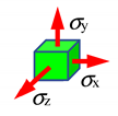 |  |  |  |  |  |
| Principal stresses | σx = σy = σz >0 | σx = σy σz = 0 | σy > 0 σx = σz = 0 | σy < 0 σx =σz=0 | −σx = −σy σz = 0 | σx = σy = σz <0 |
| ηTRIAX | ∞ | 0.66 | 0.33 | −0.33 | −0.66 | −∞ |
| Point Label | Strain | Stress | Remarks |
|---|---|---|---|
| εel, - | σtrue, MPa | ||
| 1 | 0.0040 | 605.6 | Yield point Re |
| 2 | 0.1028 | 783.8 | Ultimate tensile strength Rm |
| 3 | 0.1768 | 489.9 | Sample fracture |
| 4 | 0.2280 | 0.00 | d = 1 material total degradation |
| 5 | 0.1768 | 836.0 | Stresses in the material model without failure parameters |
| 6 | 0.1730 | 0.00 | Fracture deformation |
| 7 | 0.0991 | 0.00 | Deformation at ultimate strength Rm, d = 0 |
Publisher’s Note: MDPI stays neutral with regard to jurisdictional claims in published maps and institutional affiliations. |
© 2021 by the authors. Licensee MDPI, Basel, Switzerland. This article is an open access article distributed under the terms and conditions of the Creative Commons Attribution (CC BY) license (https://creativecommons.org/licenses/by/4.0/).
Share and Cite
Bogdan, S.; Radosław, K. Material Properties of HY 80 Steel after 55 Years of Operation for FEM Applications. Materials 2021, 14, 4213. https://doi.org/10.3390/ma14154213
Bogdan S, Radosław K. Material Properties of HY 80 Steel after 55 Years of Operation for FEM Applications. Materials. 2021; 14(15):4213. https://doi.org/10.3390/ma14154213
Chicago/Turabian StyleBogdan, Szturomski, and Kiciński Radosław. 2021. "Material Properties of HY 80 Steel after 55 Years of Operation for FEM Applications" Materials 14, no. 15: 4213. https://doi.org/10.3390/ma14154213
APA StyleBogdan, S., & Radosław, K. (2021). Material Properties of HY 80 Steel after 55 Years of Operation for FEM Applications. Materials, 14(15), 4213. https://doi.org/10.3390/ma14154213