The procedure for generating a virtual concrete mesostructure consists of two steps: (a) The generation of realistic concrete aggregate inclusions using irregular polyhedron geometries with concave depressions and (b) the packing of aggregates into the cementitious mortar (host material). The final mesostructure morphology is represented in terms of discrete voxels.
2.1. Modeling a Generic Aggregate
Coarse concrete aggregates are characterised by multiple faces, sharp corners, and irregular surfaces. Even though the shape of aggregates has a strong effect on the stress concentration, crack initiation, and propagation in concrete [
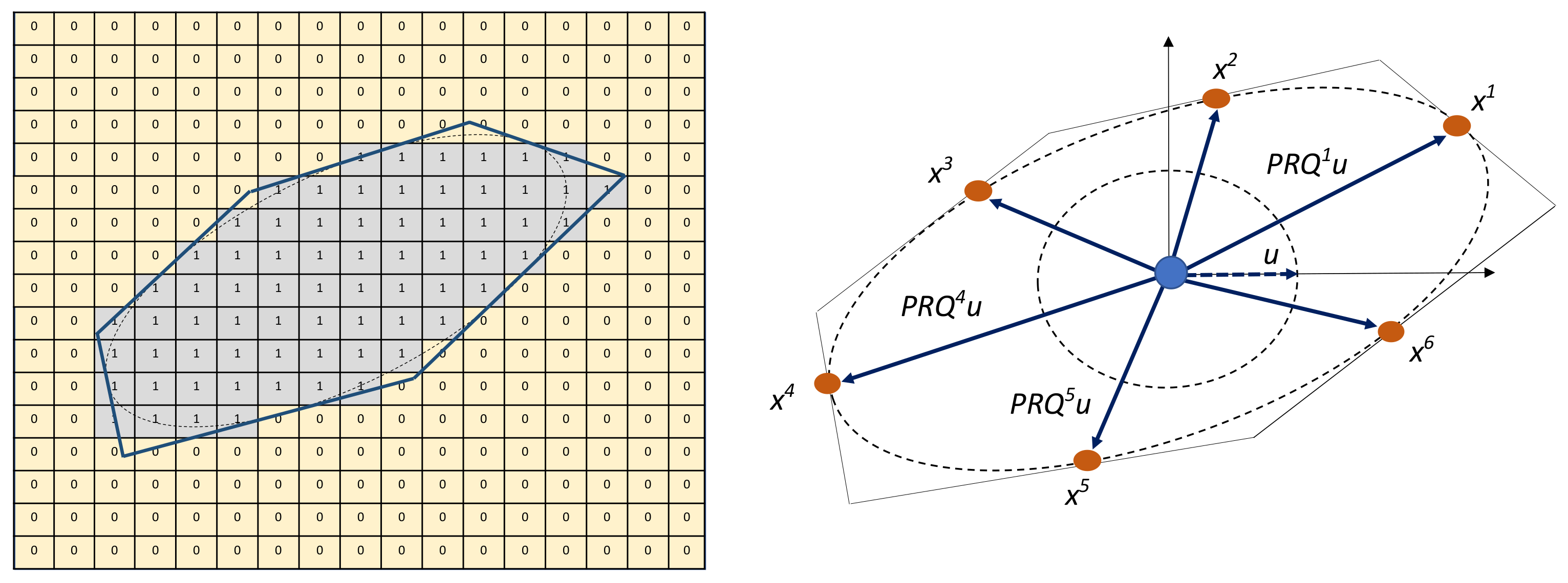
33], often oversimplified models are used in most numerical analyses. In this work, we aim at modelling the aggregate topology featuring sharpness, elongation, as well as concavity by means of an irregular polyhedron geometry. The option to include an interfacial-transition-zone (ITZ) between the aggregate and the mortar matrix is also available. The procedure to generate a virtual aggregate involves the sequential reduction of an initial cuboid to a polyhedron through slicing operations tangential to an imaginary inscribed ellipsoid as shown in
Figure 1 (left).
Given the maximum aggregate size in mm, we generate a 3D array of voxels of dimension . Here, and is rounded-off to the nearest integer and its dimension is [voxels]. The parameter h [mm/voxel] is the resolution of the virtual mesostructure generated by the CMG. h is used to convert physical dimensions in SI units into voxels, its value can be set depending on the available computational resources. If l is an even number, then l is incremented by one. This is to ensure that the array contains a mid-point voxel. The voxel at the mid-point of the array at position is set as the origin for a cartesian coordinate system in voxel coordinates.
In order to model flat and elongated aggregates, we introduce the aspect-ratio
. Given the aspect-ratio and the voxel dimensions
l, we first inscribe an imaginary ellipsoid with dimensions
. Then, the required number of faces
N on the polyhedron representing the aggregate is specified. Subsequently,
N points, denoted by the position vector
, which are located on the surface of the inscribed ellipsoid are chosen randomly (see
Figure 1 (right)). The faces of the polyhedron are assumed to be tangential to the inscribed ellipsoid at these points. Each tangent plane
i is defined using a planar equation, which is a function of the point
and orientation angles
,
, and
. The position vectors
are determined as:
with
denoting a unit vector. The rotation operator
with angles
,
, and
determines the final orientation of the polyhedron, and the rotation operator
with angles
,
, and
determines the orientation of a polyhedron face
i. The rotation angles
,
, and
are chosen randomly, as aggregates in concrete do not in general orient themselves along a certain axes.
is a matrix that specifies the dimensions of the ellipsoid. All geometrical operations are performed using real numbers. After having specified the final geometry of the aggregates, we round-off the real number to the nearest integer that corresponds to the discrete voxel positions. The complete expressions for the operators introduced in Equation (
1) are given below:
where
, and
.
In order to perform the imaginary cutting operation (sequential reduction of the cuboid to a polyhedron), all voxels with position vectors
are set to one if they satisfy the following condition:
Here,
for
is the surface of the ellipsoid at
. The above expressions are evaluated at all voxel positions. The position of the
kth voxel is denoted as
. (It should be noted, that
is rounded to the nearest integer before performing the calculations.)
Figure 1 (left) shows an illustration of a section of the 3D array after having performed the aforementioned operations.
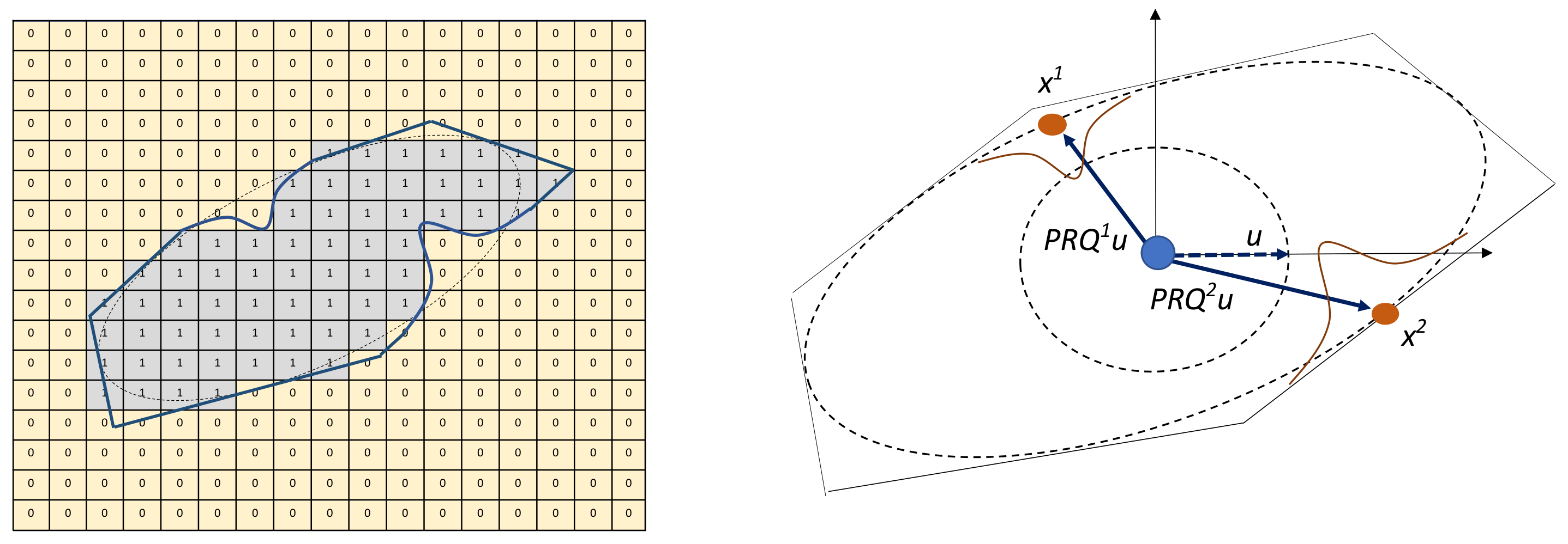
Certain aggregate geometries are characterised by concave depressions, e.g., from crushing the aggregates during the production process. So far, we have designed a polyhedron whose geometry is described by voxel value = 1 embedded in a matrix material with voxel value = 0. Certain volumes of the voxel can be sculpted out to introduce concave depressions. This translates to replacing certain voxels with value 1 that are inside the volume to be sculpted out to 0. Concave depressions are introduced on the inscribed ellipsoid using the Gaussian surface equation (see
Figure 2, right). The condition for setting a voxel to zero is specified as:
where
M denotes the total number of concave depressions centered at
. This equation implements a Gaussian surface below the ellipsoidal surface and checks if the voxel value is zero or not. Here
are computed from Equation (
1). The width of the Gaussian surface is
w, the depth is
d, and
is the variance parameter (see
Table 1 for more details). Concave depressions are generated on the surface of the imaginary ellipsoid at random locations.
The procedure is as follows: First,
M number of positions
for the Gaussian surface are generated. Using these positions, the concave equations (Equation (
3)) are generated with the input parameters
d and
w, which control the depth and width of the concavity from the ellipsoid surface. The voxel values of the points which lie inside the polyhedron and below the Gaussian surface are changed from zero to one as shown in
Figure 2.
is rounded to the nearest integer before performing the calculations and
are the voxel positions.
A summary of all parameters for the generation of realistic generic aggregates are provided in
Table 1.
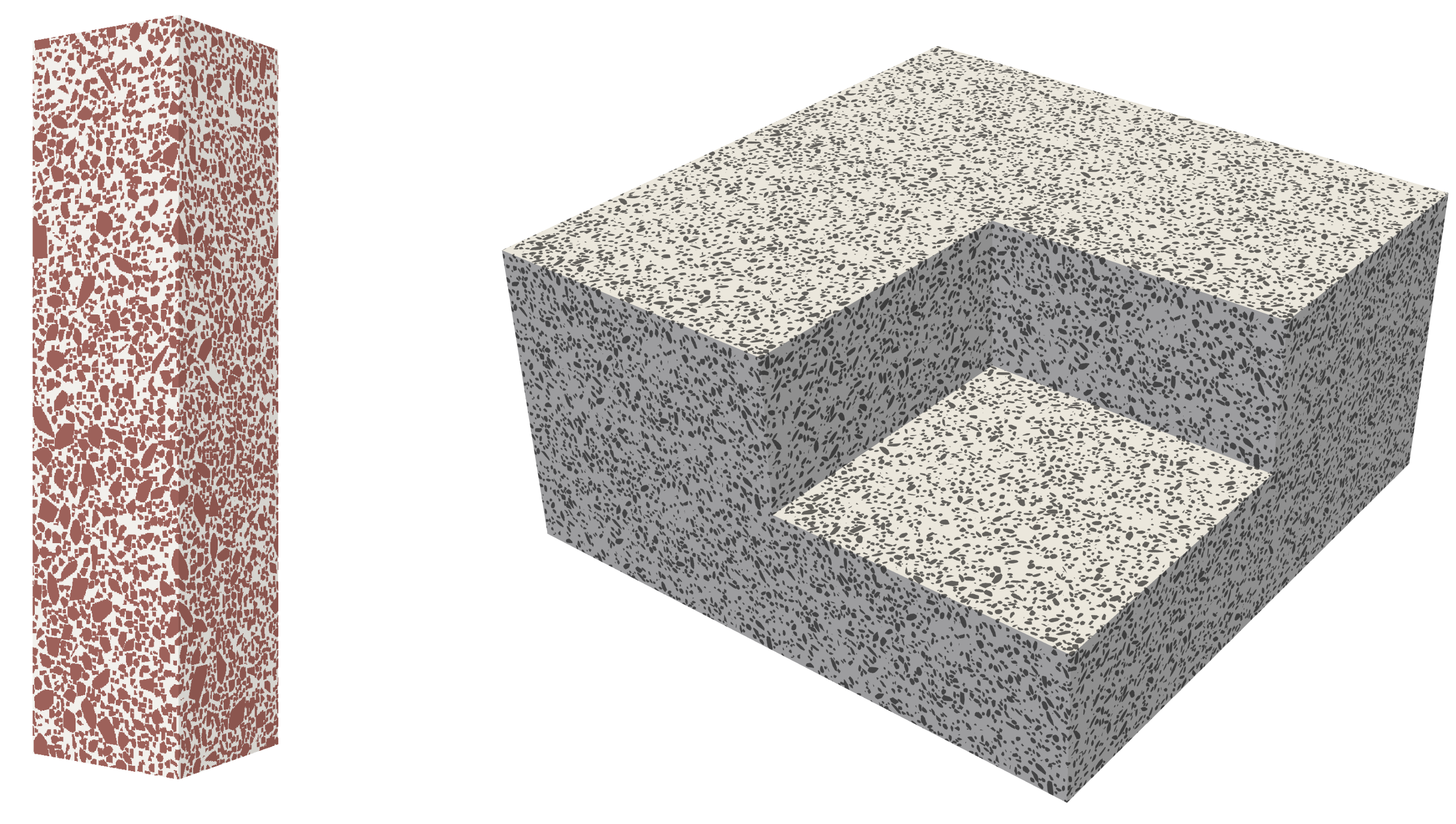
In order to include the ITZ as a coating around the aggregate, the thickness
t of the ITZ is the only input. The algorithm uses the same technique as that of the polyhedron and the Gaussian surface, but with a larger concentric imaginary ellipsoid. The thickness
t is added to the polyhedron ellipsoid axes to obtain the coating surface,
Hence, there will be two sets of concentric polyhedron and Gaussian equations. The final algorithm checks for all points in the domain first for the outer surface followed by the inner surface. Voxels at the ITZ are represented with voxel value 2. This methodology can also be used to enforce a minimum spacing between the aggregates by setting these voxel values equal to that of the matrix (host) material.
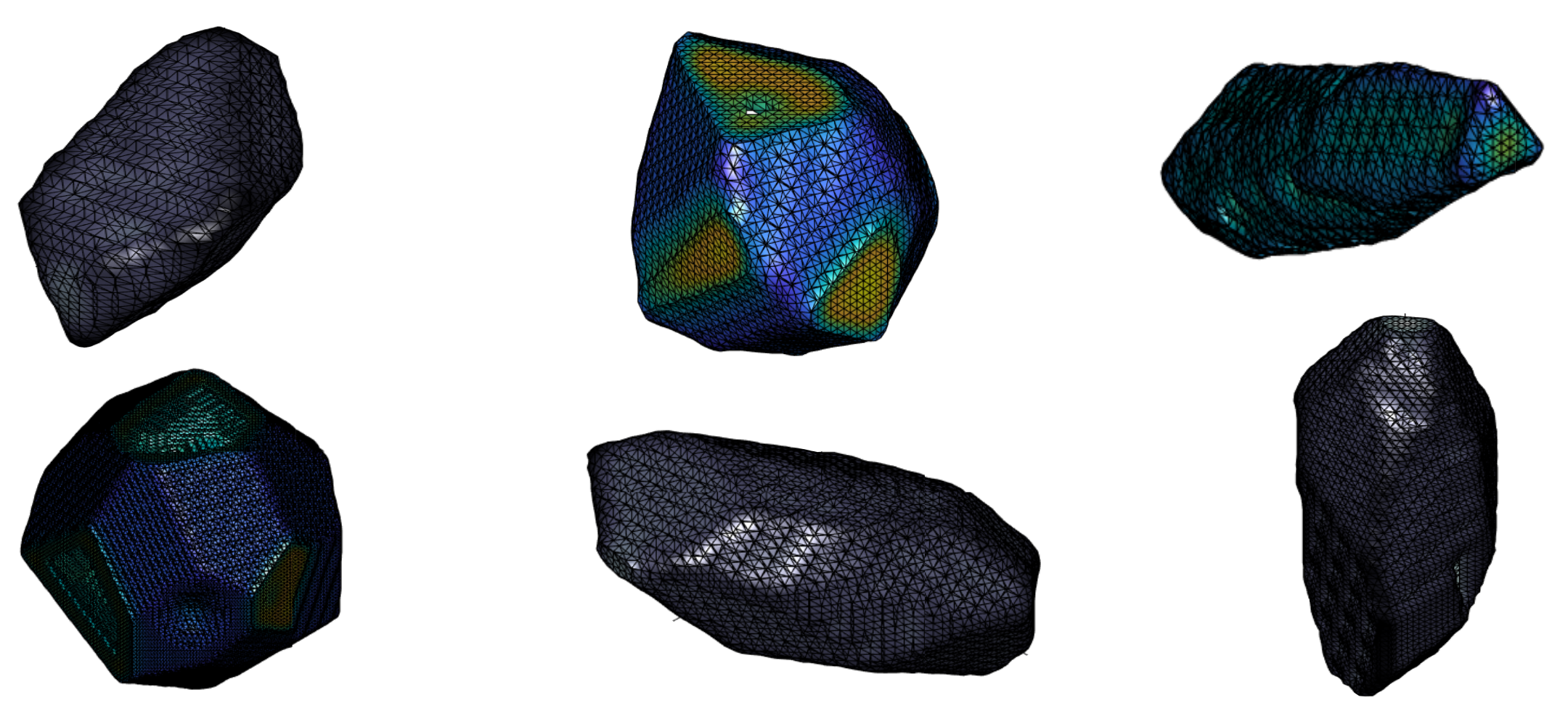
Figure 3 shows aggregate samples generated by the aforementioned procedure. For a better visualisation, the surface region of the aggregates is smoothed. With multiple irregular surfaces, different aspect ratios, and concave depressions, it can be seen from these samples that the proposed algorithm can generate realistic aggregate geometries.
Figure 4 shows aggregates in their original voxel form with and without a layer representing the ITZ (in red).
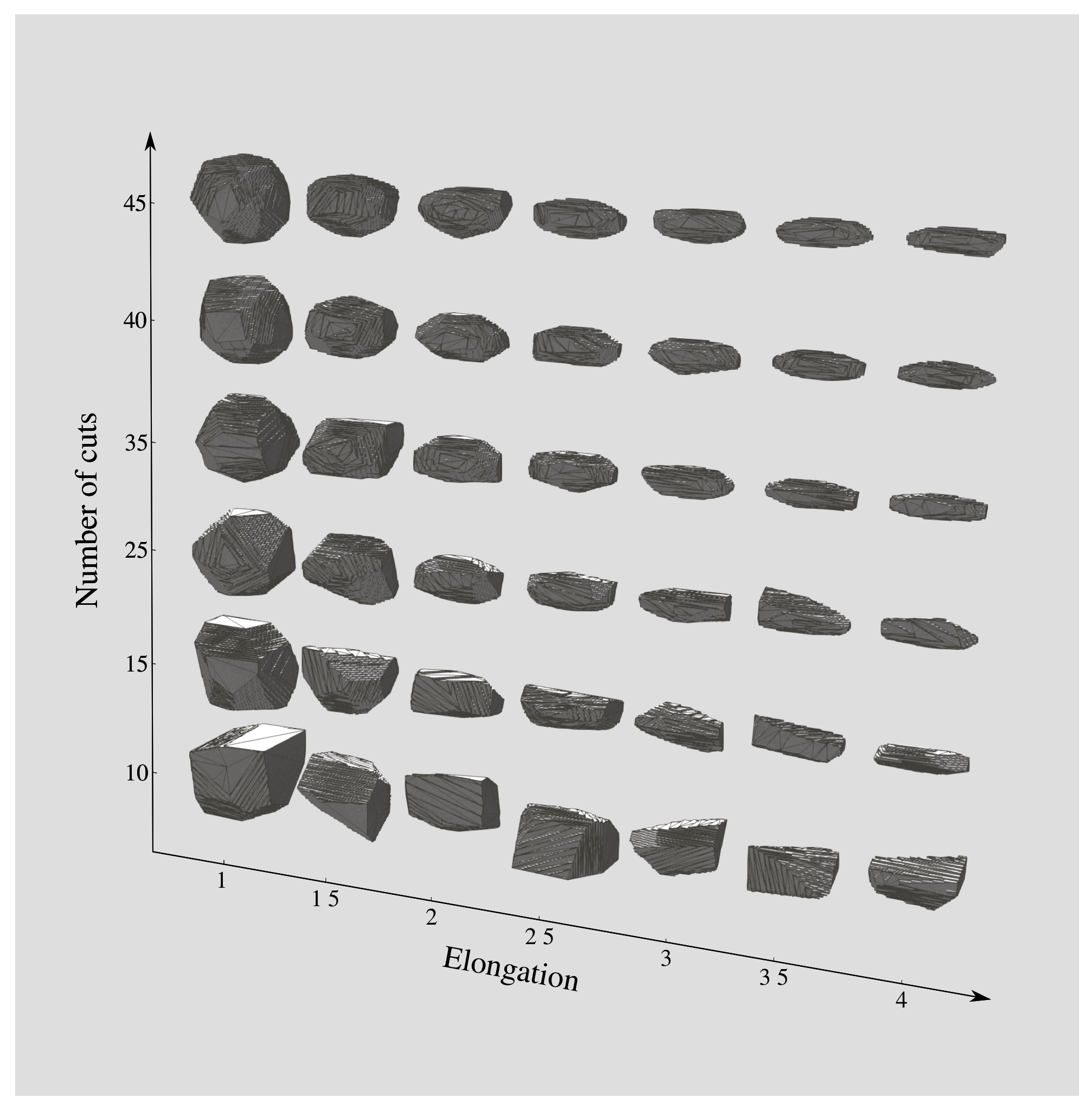
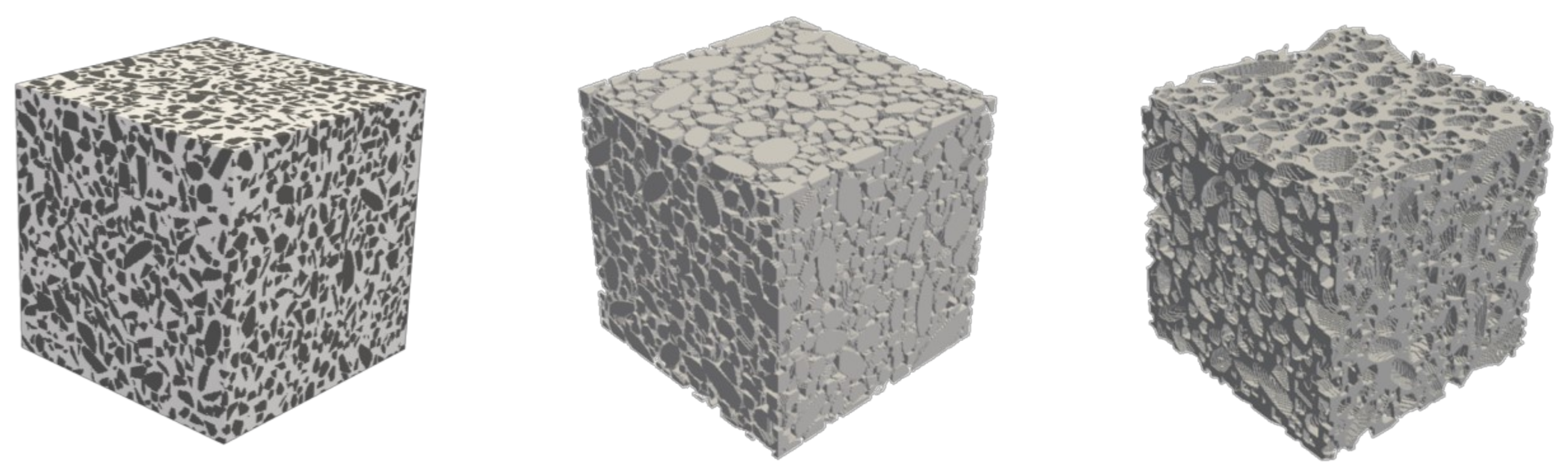
Figure 5 shows the effect of the number of polyhedron faces
N and the elongation (
) on the aggregate shape. The aggregate size
l of all aggregates is set to 50 voxels. The elongation varies from 1 to 4, while the number of cuts varies from 10 to 45. The aggregates are visualised using the open-source software Paraview using the decimate filter. By varying the number
N of cuts and the aspect ratio
, we can obtain different types of concrete aggregates ranging from smooth-surfaced pebbles to sharp-edged aggregates that can be spherical, flat, or elongated.
2.2. Generating a Concrete Mesostructure
Once the aggregate is generated, it is assembled into the concrete mesostructure with a mortar matrix. The mesostructure includes both the mortar host material and aggregate inclusions in voxel format. At a given voxel position, the mortar host phase is represented with value zero and the aggregate phase with a non-zero value. The size of the voxel domain can be varied based on the requirement of the resolution and size of the mesostructure. The CMG assembly algorithm first initialises a voxel domain to the required size (
,
,
) rounded to the nearest integer filled with voxels of zeros representing the mortar host phase. Then, inclusions are generated using the aforementioned aggregate generation procedure and assembled into the domain. The basic requirements of a packing algorithm (see for e.g., [
34,
35]) are as follows: (a) Ensuring that the aggregates do not overlap, (b) ensuring random spatial distribution, (c) providing maximum packing density, and (d) that the mesostructure at the boundaries must be periodic.
The random sequential adsorption (RSA) algorithm [
36] is used as the basis for the assembly procedure. In this algorithm, starting with the homogeneous voxelised domain, representing the mesostructure containing only the host phase, inclusions are generated and randomly placed in the domain. A random location from the 3D domain is identified and an attempt is made to include an aggregate (also in voxel format) at this location. The aggregate candidate is embedded into the current domain if there is no overlap of the aggregates. To check for overlapping, one-to-one comparison of the voxels between the inclusion matrix and that of the mesostructure matrix at the proposed assembly location is made. If all the voxels at the assembly location in the mesostructure matrix have the value of zero, then assembly is executed. According to the original RSA algorithm, if there is interference with an already assembled aggregate, a new random point is chosen and the same procedure is repeated until the particle finds a new position without any overlap with other aggregates. Once assembled, the same procedure is repeated for the newly created aggregate inclusion until the required maximum volume fraction of each inclusion size is achieved. To achieve the fastest possible assembly and higher packing density, the aggregates are assembled sequentially in a hierarchic manner according to the aggregate size from largest to smallest.
As the hosting domain is incrementally populated with aggregates, the probability of finding free space to embed a new aggregate becomes increasingly small. In the original (sub-optimal) MATLAB implementation of the model, the RSA algorithm, even though it generates statistically equivalent mesostructures by randomly distributing the aggregates in the mesostructure, achieving a packing density of more than 30%, requires a significant time for computations since the assembly procedure is completely random. Hence, to achieve a higher packing density in less computation time, the algorithm was modified from a random to a semi-random assembly algorithm (SRSA). According to SRSA, if the aggregate to be assembled does not find free space in the current random position, instead of finding a new random position, the current aggregate is incrementally translated along an orthogonal plane (either
or
) until the non-overlapping condition is fulfilled. SRSA was four times faster than the RSA algorithm in the Matlab implementation. However, in the current Python implementation available in [
37], we observed no significant speed up as the base code was already significantly improved and optimised.
The assembly algorithm also implements periodic boundary conditions.
Figure 6 shows typical concrete mesostructures showing the aggregate phase, the mortar matrix phase, and the concrete mesostructure generated by the CMG. The parameters used to generate this mesostructure are presented in the following section.
2.3. Data for the Calibration of the CMG
At the mesoscale, the internal material structure of concrete is characterised by a large volume fraction of aggregates (up to 60–70%) of different sizes, embedded in the cementitious matrix. One of the most conventional aggregate size distribution curves is that of standard DIN-1045 or the Fuller curves. As a result, a realistic virtual concrete sample should statistically represent such a distribution. To this end, the concrete standard AB16 (according to DIN-1045) with the largest aggregate size of 16 mm is considered. The voxel size is chosen to be 0.5 mm, i.e., the parameter corresponding to the resolutions . Only coarse aggregates of a size larger than 3 mm onwards are explicitly resolved. The fine aggregates are embedded in the hardened cement paste to form the mortar material.
A detailed quantification of aggregate size distribution for AB16, together with the measurement of elastic properties of the investigated concrete samples was performed in the laboratory. The aggregates size distribution obtained from the measurements is summarised in
Table 2. This data serves as the direct input for the packing algorithm, resulting in a total aggregate volume fraction of 48.29% that will be explicitly resolved.
The procedure for the calibration of the parameters defining the morphology of the aggregates is as follows: For each particle, the two most important parameters are the aspect ratio and the number of faces of the polyhedron N. As it was found that the aggregates of a larger size exhibit a wider range of aspect ratio, the aspect ratio of aggregates greater than 8 mm is randomly chosen from 1.75 to 3.25. Similarly, the aspect ratio range of aggregate sizes from 4 mm to 8 mm is within 2 to 3 and for a size of 3 mm, it is within 1 to 2. The number N for each size is determined by multiplying the aggregate size (in terms of voxel) by a factor whose value is either 0.5 or 0.625. It is to be noted that this range of values was chosen after performing several trials to obtain a realistic geometry. With regards to the concave depression in the aggregates, only aggregates larger than 12 mm are assumed to exhibit such a feature, with the prescribed values of 5 concave surfaces, 3 mm in width, and 2.5 mm in depth per aggregates particle. The variance parameter of the surface was chosen as . This choice of value provided the most realistic concave depressions for the considered aggregate sizes. For each successful placement of an aggregate, statistical data, such as volume fraction and number of particles of each size, are recorded as a footprint of the numerical sample. CMG can also be used as a tool for testing a certain distribution of aggregates before the actual production of concrete samples.
2.4. Comparison of Simulations vs. Laboratory Measurements
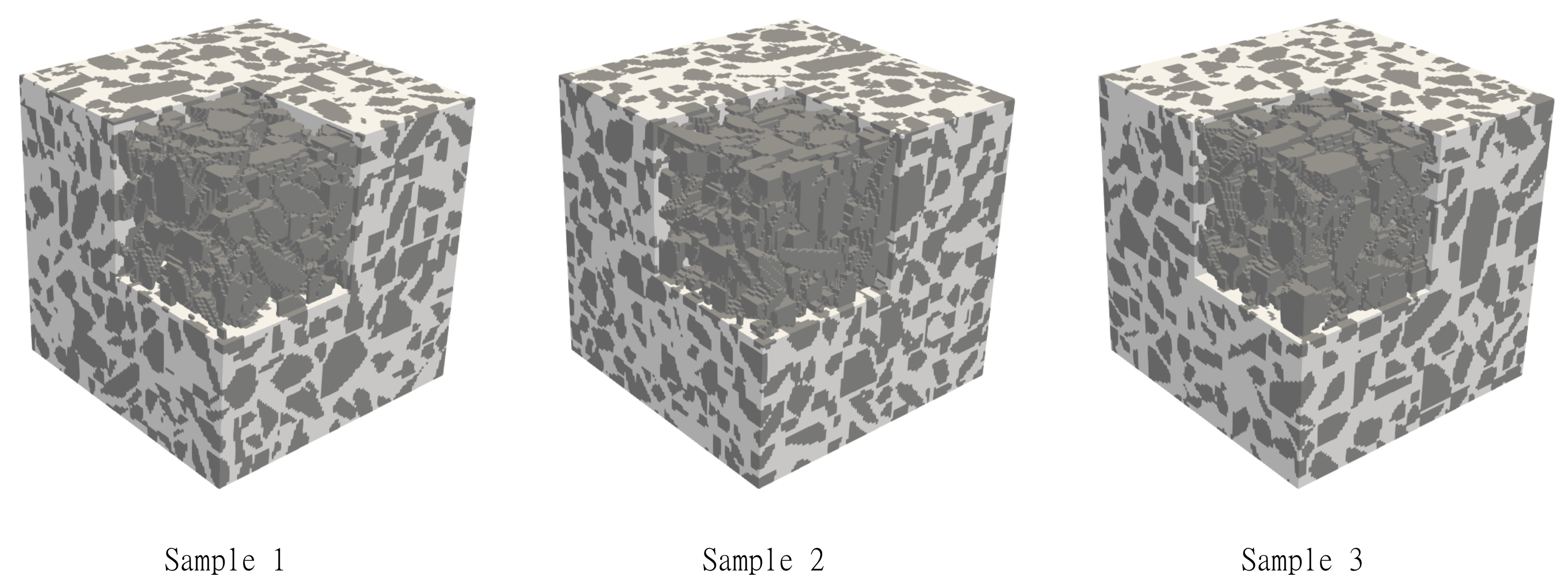
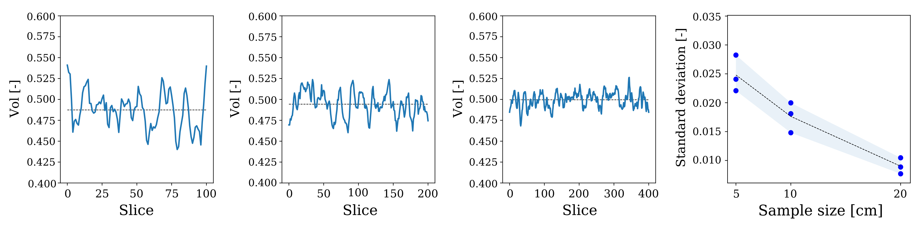
In order to test the capability of the method to generate virtual AB16 mesostructures using the data from the previous section, three sample sizes of 5, 10, and 20 cm were considered. From each sample size, three specimens are generated to capture the possible stochastic fluctuation of the samples, analogous to experimental practice. The visualisation of each size is shown in
Figure 7, together with the statistical information, number of particles, and volume distribution with respect to particles size. It can be seen that, in most samples, the distribution curve is in agreement with the actual grading curve obtained from laboratory measurements. The average total number of particles for each size are 1039, 7838, and 62,553 particles. The total volume fraction of these nine specimen range from 47.3% to 49.95% due to the stochastic nature of the random operations, which is acceptable, considering the computational efficiency and large number of aggregates.
Figure 8 shows the actual concrete mesostructure image (Left) compared with the virtual mesostructure image (Right) generated by the CMG. Comparing the aggregate shapes, orientations, and distributions, the mesostructure image from the CMG and the actual concrete image are very similar. We can observe in both the images that the particle shapes range from an almost circular surface to highly elongated sharp-edged surfaces and that the packing density varies from less concentrated aggregate regions to densely packed regions. One can also observe concave depressions on actual concrete image similar to the CMG mesostructure.
Figure 9 shows large-sized virtual concrete mesostructures according to the AB16 standard with a maximum aggregate size of 16 mm.
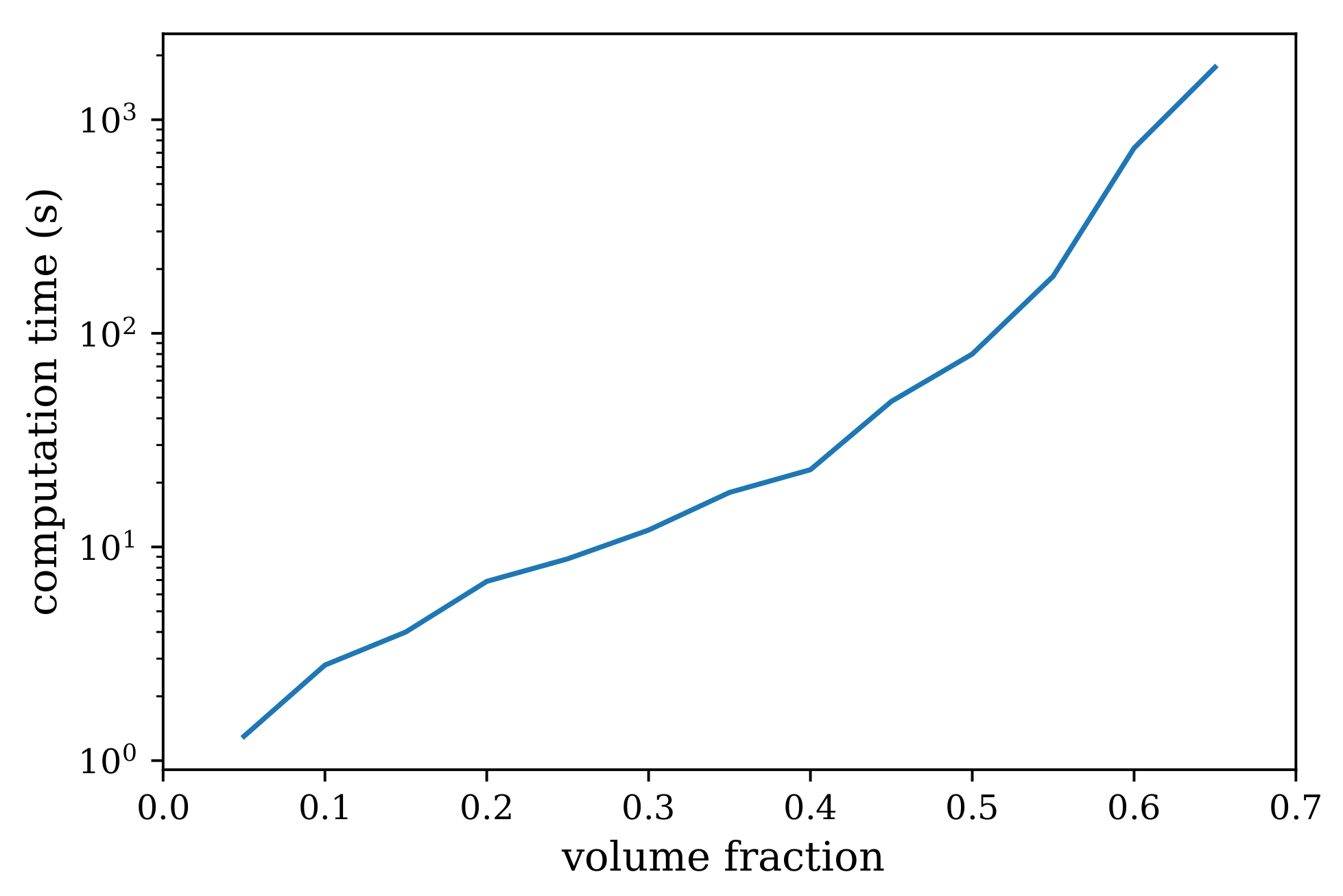
The time required for generating a mesostructure of resolution
on a 6-year-old Intel(R) Core(TM) i5-4210U CPU @ 1.7 GHz laptop for various volume fraction of aggregates is shown in
Figure 10. Computation times are hardware specific and the values shown here are expected to be the lower bound on the expected time for generating a virtual mesostructure using PyCMG [
37].


 ,
, 


