Decoding Rocks: An Assessment of Geomaterial Microstructure Using X-ray Microtomography, Image Analysis and Multivariate Statistics
Abstract
1. Introduction
2. Materials
3. Methods
3.1. Polarized Light Microscopy and Cathodoluminescence
3.2. X-ray Microtomography
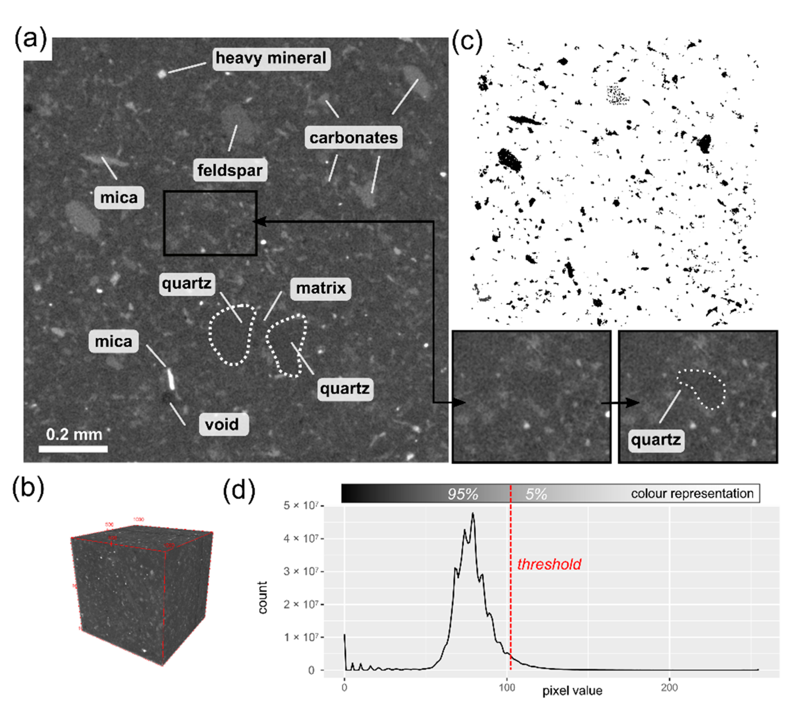
3.3. Image Processing and Analysis
3.4. Exploratory Data Analysis
3.5. Cluster Analysis
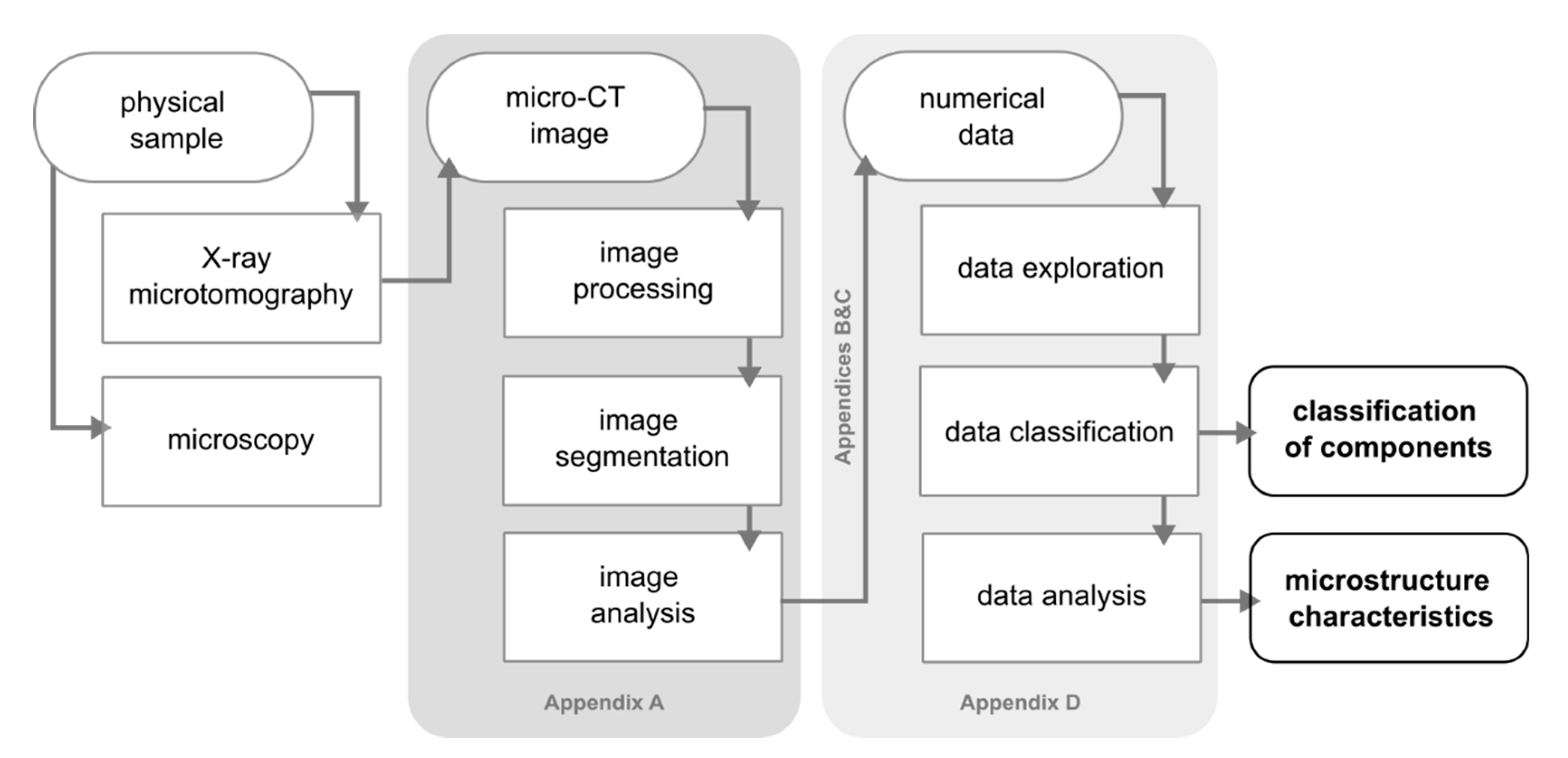
3.6. Microstructure Assessment
4. Results
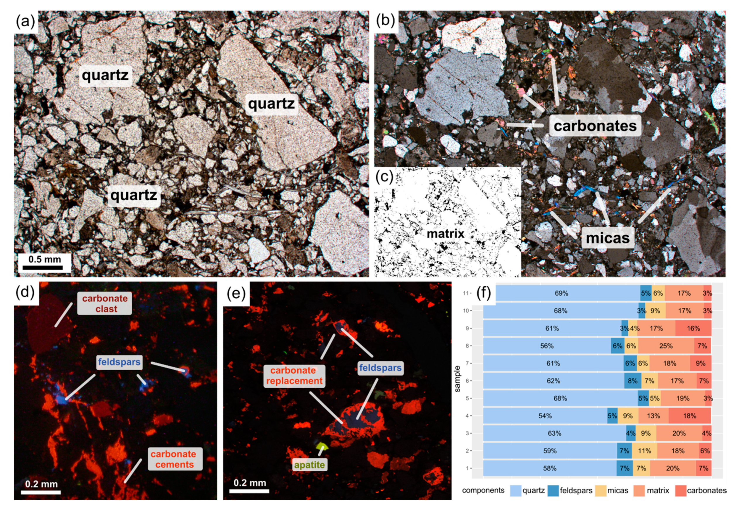
4.1. Sample Characterization
4.2. Data Exploration
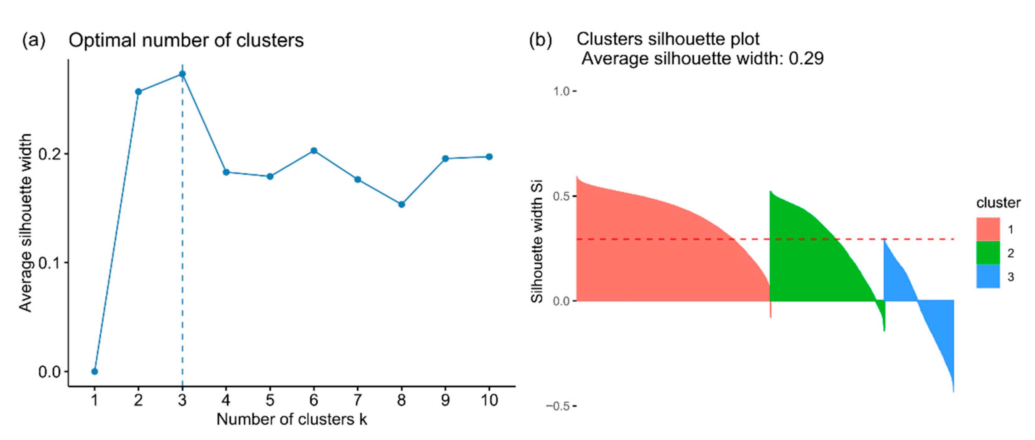
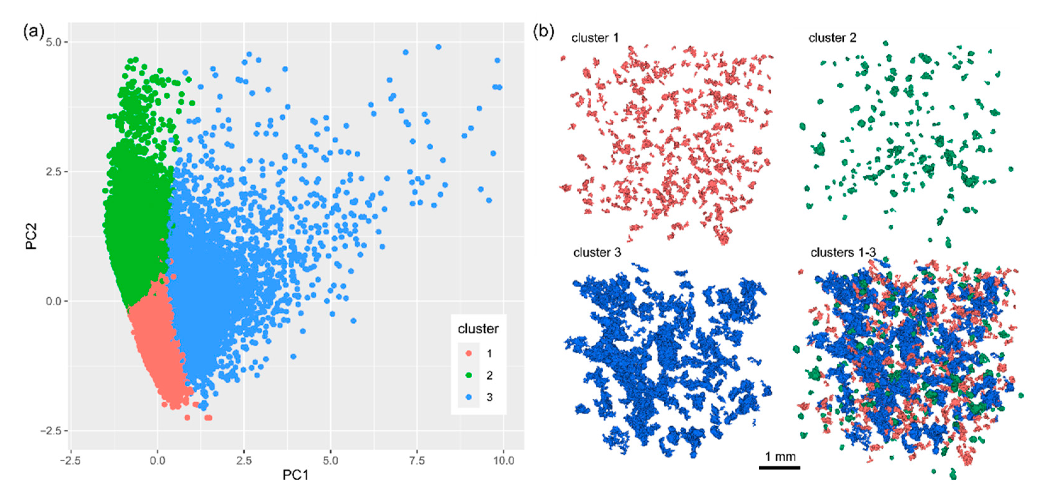
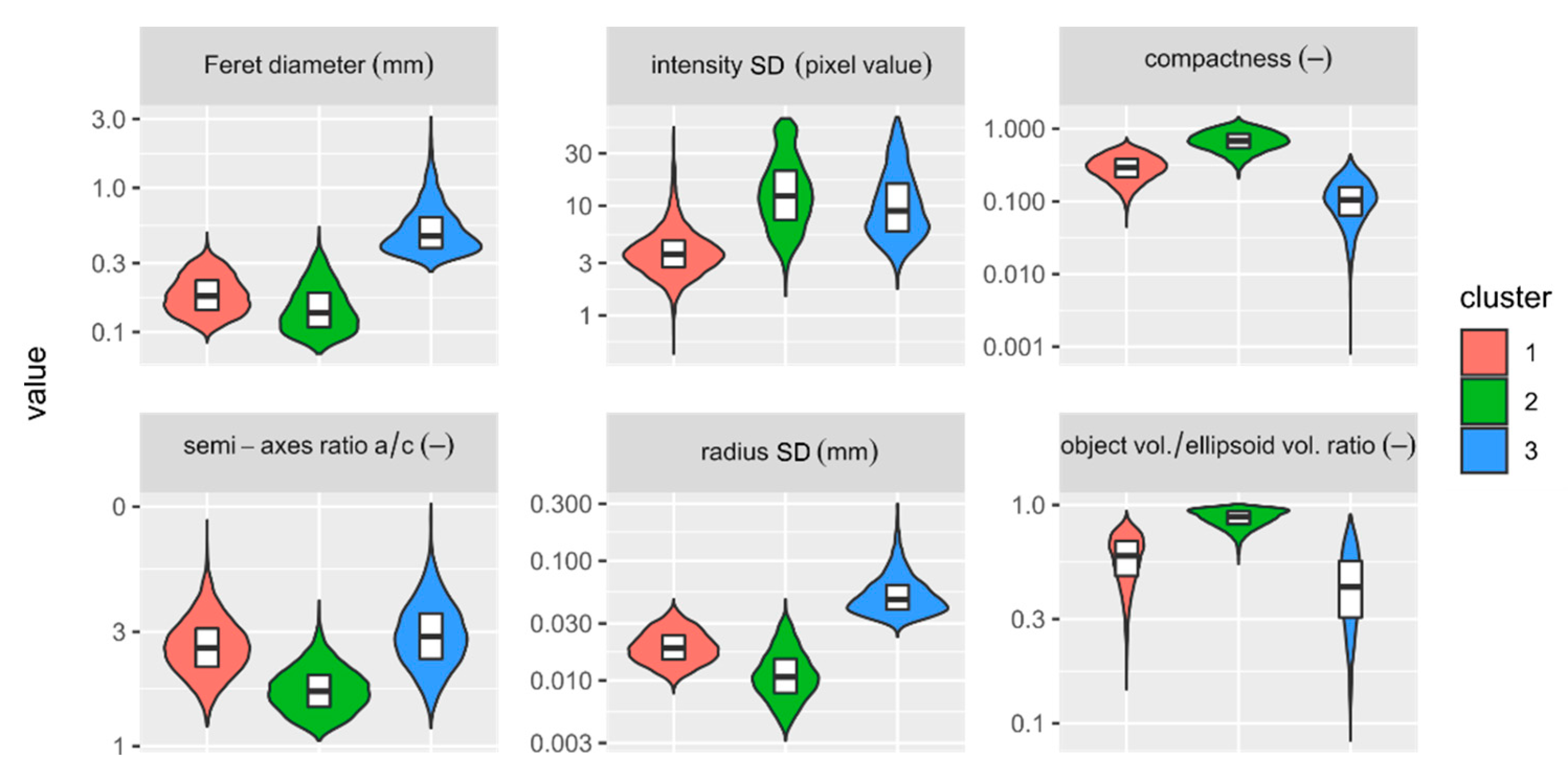
4.3. Classification of Components
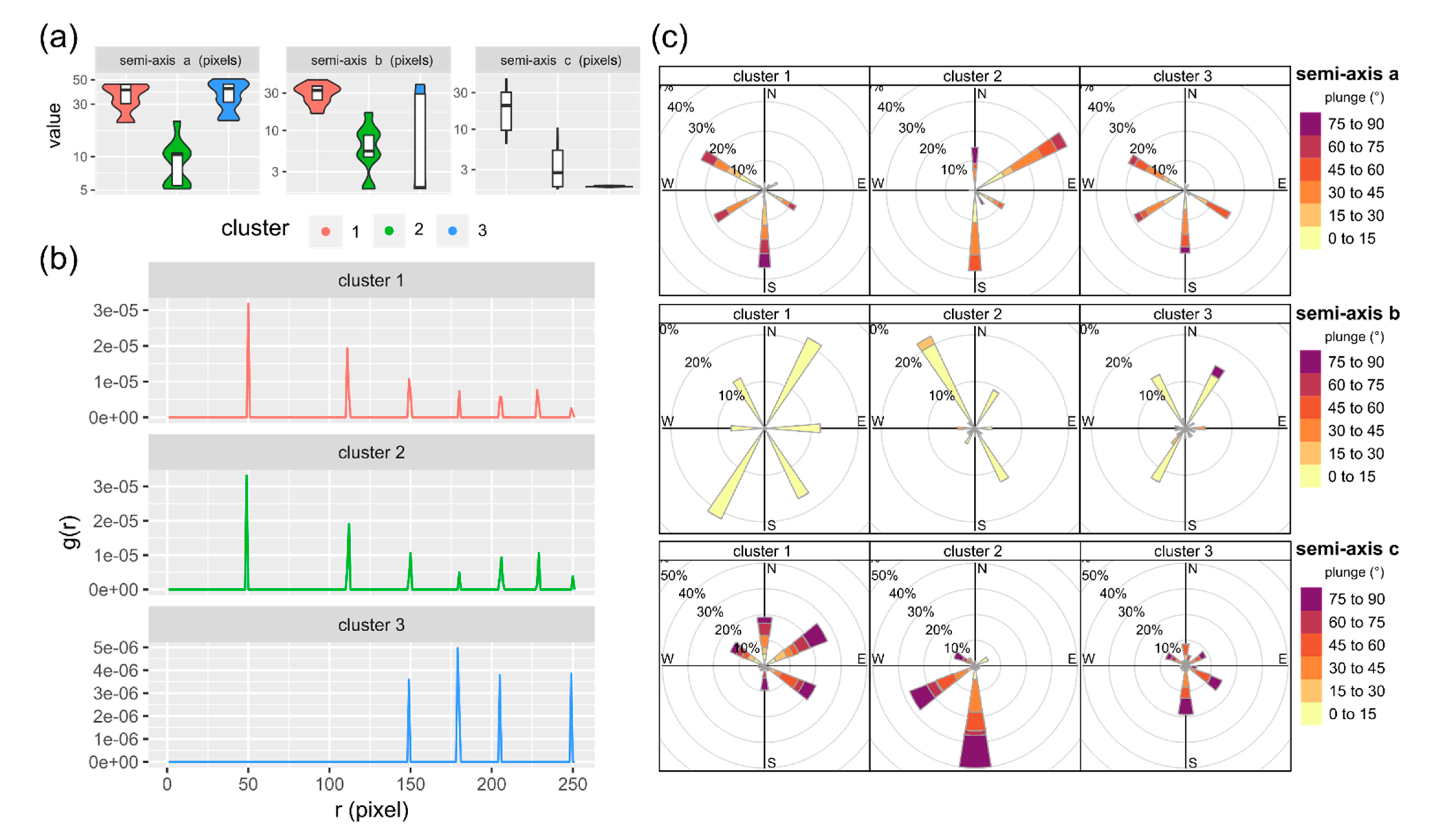
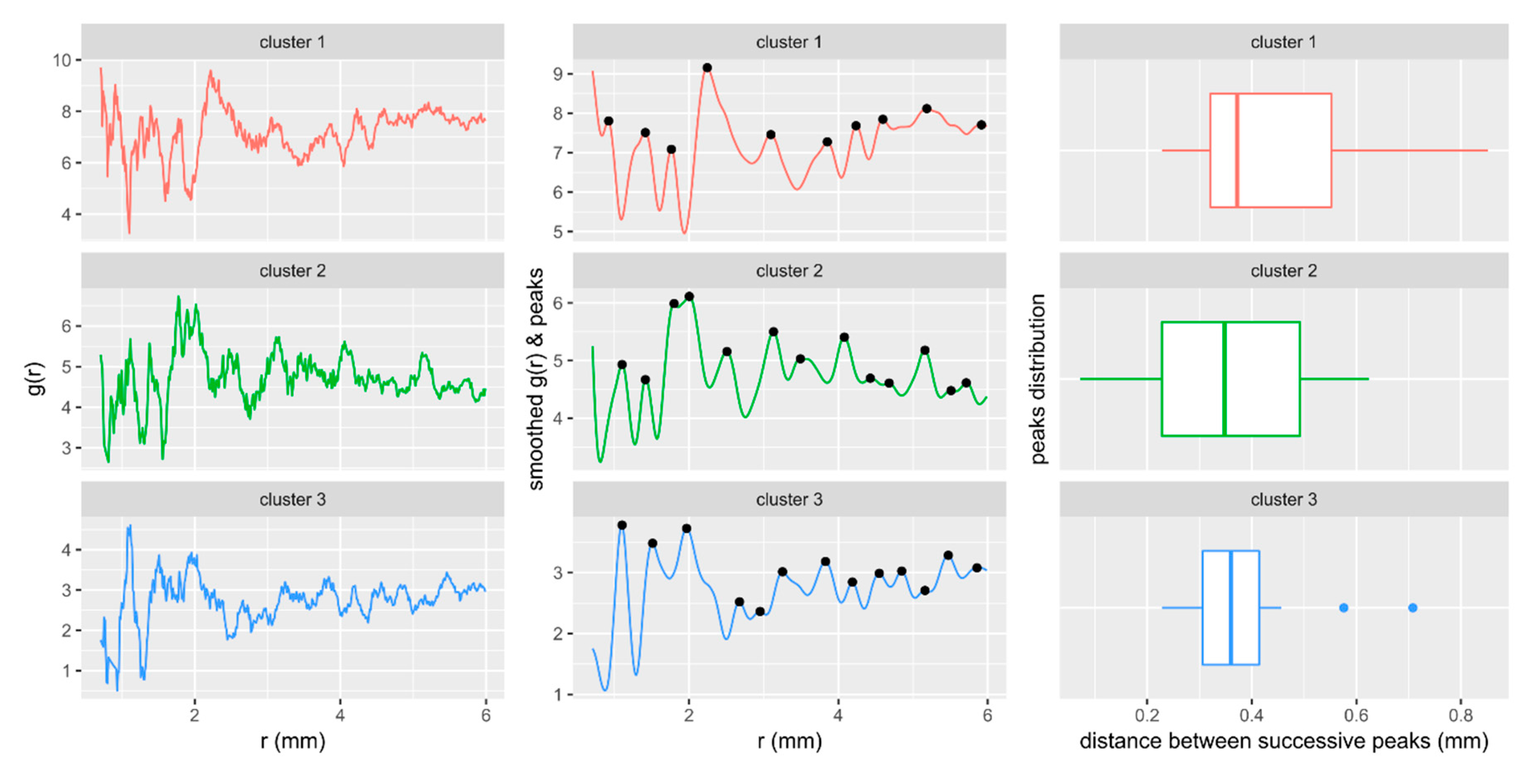
4.4. Microstructure Assessment
5. Discussion
5.1. Image Processing and Analysis
5.2. Data Exploration
5.3. Data Classification
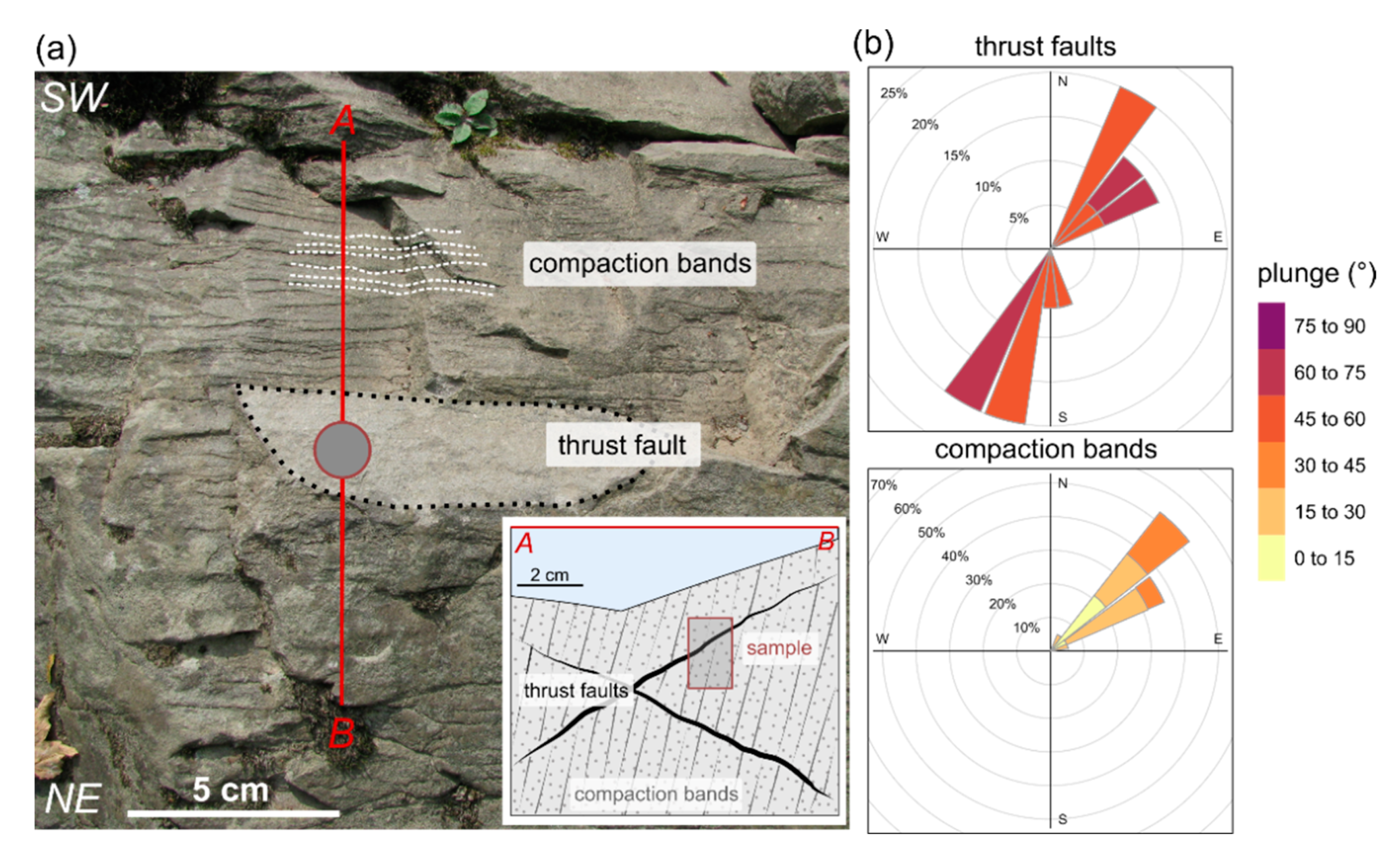
5.4. Microstructure Interpretation: A Case Study
6. Summary and Conclusions
Author Contributions
Funding
Institutional Review Board Statement
Informed Consent Statement
Data Availability Statement
Conflicts of Interest
Appendix A. The Protocol of Image Processing and Analysis in Fiji
- 1.
- Launch Fiji Software
- 2.
- File > Open # open a micro-CT image - read into RAM (File > Import > TIFF Virtual Stack – read an image directly from drive storage)
- Image processing
- 3.
- Image > Type > 8-bit # convert image to 8-bit type
- 4.
- Image > Crop # resize and crop the image
- 5.
- Image > Adjust > Brightness/Contrast # adjust brightness and contrast
- 6.
- Plugins > BaSiC # apply a X-ray attenuation correction
- 7.
- File > Save As > Tiff # save the corrected image
- 8.
- Image > Adjust > Threshold > * (check stack histogram) > Apply > * (uncheck calculate threshold for each image) # choose and extract chosen components to a binary image format at appropriate threshold level
- 9.
- Plugins > 3D > 3D Fast Filters > * median # apply 3D median filter on the binary image
- 10.
- Plugins > MorphoLibJ > Kill Borders # remove objects at the edges of the image
- 11.
- Plugins > MorphoLibJ > Binary Images > Size opening 2D/3D # remove objects below chosen size
- 12.
- Plugins > 3D > 3D Simple Segmentation # assign ID to each separate object
- 13.
- File > Save As > Tiff # save the segmented image
- Image analysis
- 14.
- Plugins > MorphoLibJ > Analyze > Analyze Regions 3D > * File > Save As > regions.csv # perform and save the measurements; the segmented image is required
- 15.
- Plugins > MorphoLibJ > Analyze > Equivalent Ellipsoid > * (eigenvectors table) File > Save As > eigenvectors.csv # perform and save the measurements; opened the segmented image is required
- 16.
- Plugins > MorphoLibJ > Analyze > Geodesic Diameter 3D > * File > Save As > geodesic.csv # perform and save the measurements; the segmented and corrected images are required
- 17.
- Plugins > MorphoLibJ > Analyze > Intensity Measurements 2D/3D > * File > Save As > intensity.csv # perform and save measurements, opened the segmented and corrected images are required
- 18.
- Plugins > 3D > 3D Manager > * Settings > * (in the measurements section check all but Convex Hull) > OK > Add Image > Select All > Measure 3D * File > Save As > measure.csv # perform and save the measurements; the segmented image is required
- Data visualization
- 19.
- Plugins > MorphoLibJ > Binary Images > Assign Measure to Label # assign values from a table to the objects in the segmented image i.e., cluster id. (Open > clusters.csv)
- 20.
- Plugins > 3D Viewer # visualize the image in 3D
Appendix B. The Code for Raw Data Processing and Data Set Preparation
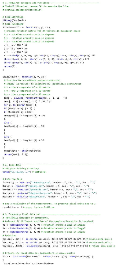
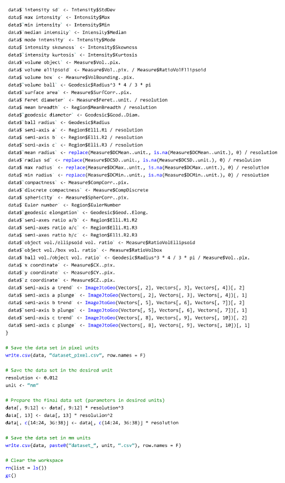
Appendix C. Data Description and Manipulation
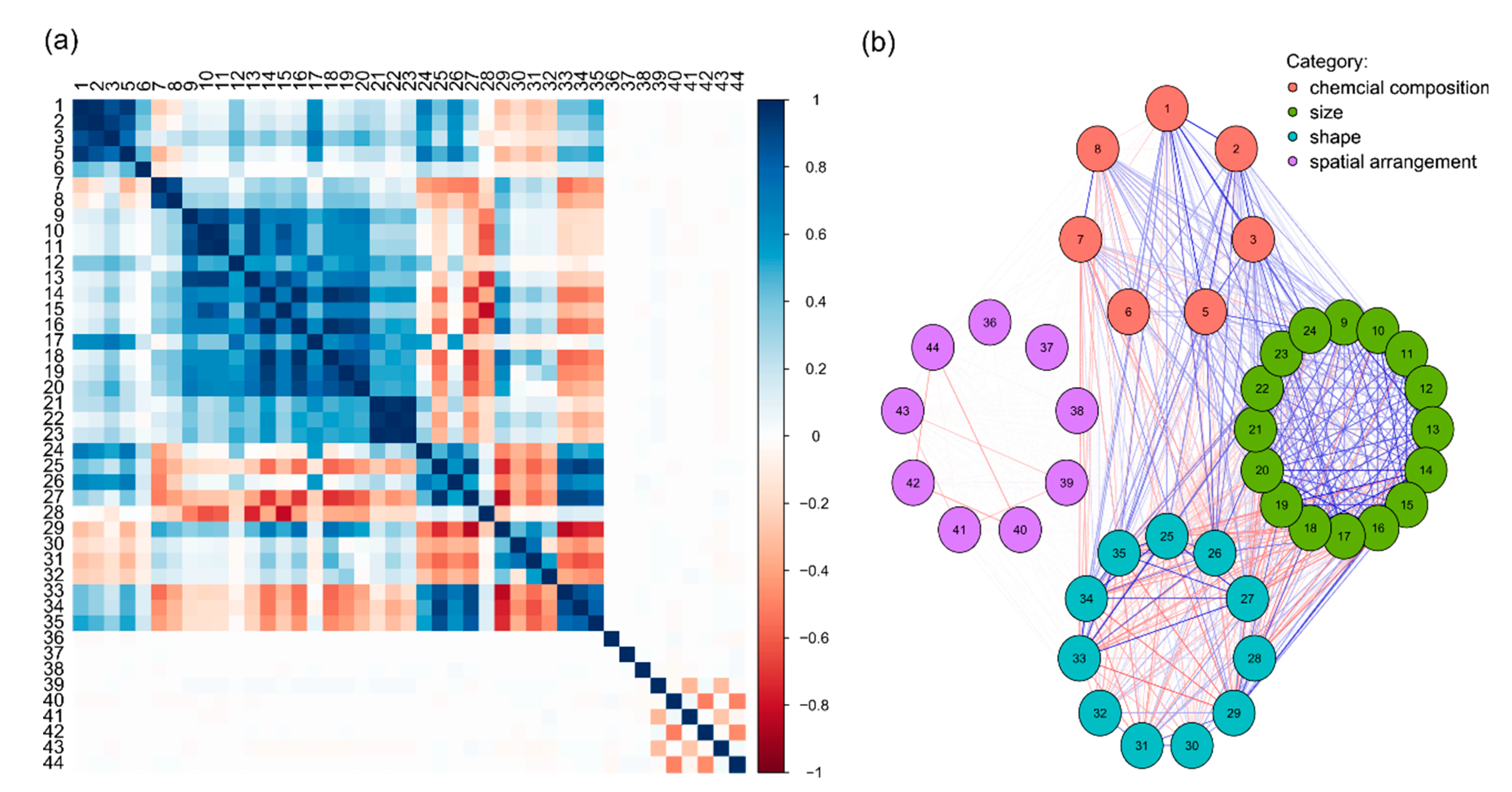
| Category | No. | Parameter | Description |
|---|---|---|---|
| Chemical Composition | 1 | mean intensity | mean of voxel values in the object |
| 2 | intensity SD | standard deviations of voxel values in the object | |
| 3 | max intensity | maximum of voxel value in the object | |
| 4 | min intensity | minimum of voxel value in the object | |
| 5 | median intensity | median of voxel values in the object | |
| 6 | mode intensity | mode of voxel values in the object | |
| 7 | intensity skewness | the skewness of voxel values distribution in the object | |
| 8 | intensity kurtosis | kurtosis of voxel values distribution in the object | |
| Size | 9 | object volume | the volume of the object |
| 10 | ellipsoid volume | the volume of the ellipsoid fitted to the object | |
| 11 | box volume | the volume of the bounding box encompassing the object | |
| 12 | ball volume | the volume of the largest ball inscribed in the object | |
| 13 | surface area | the sum of the surface area of contouring voxel faces | |
| 14 | Feret diameter | the largest calibrated distance between two contour voxels in the object | |
| 15 | mean breadth | the mean of the Feret diameter measured in all directions of the object | |
| 16 | geodesic diameter | the length of the longest geodesic path within the object | |
| 17 | ball radius | the radius of the largest inscribed ball | |
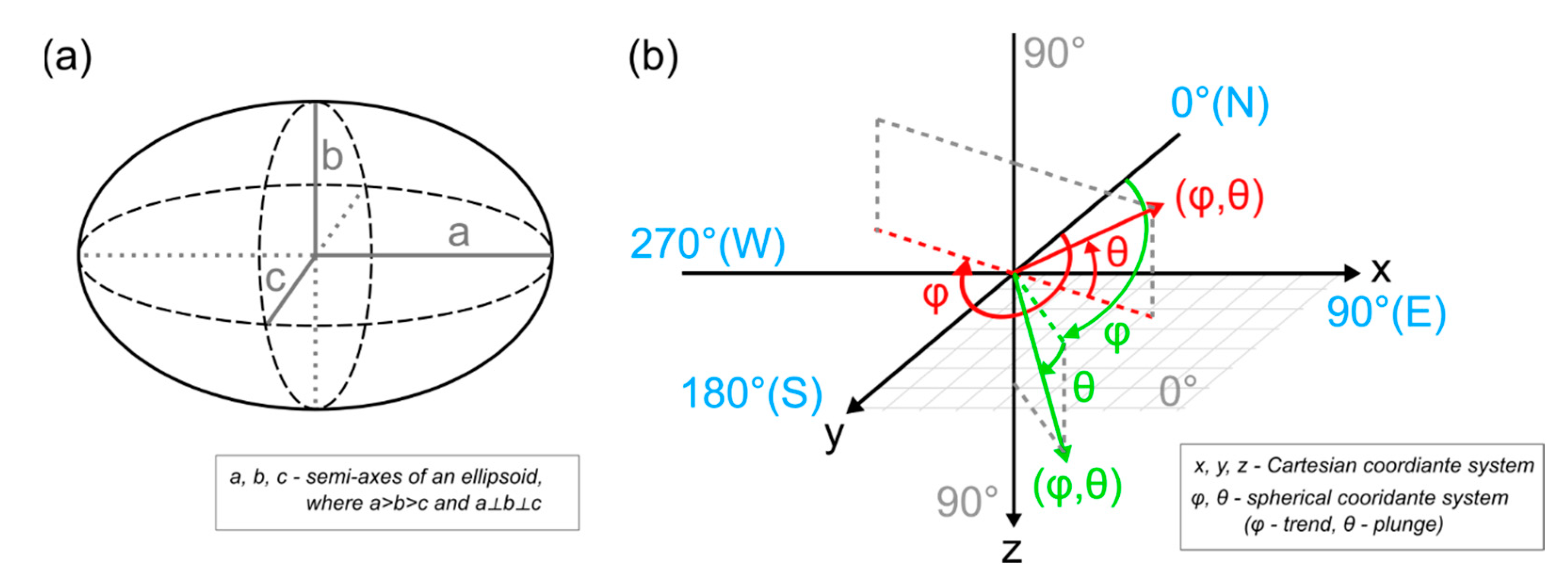
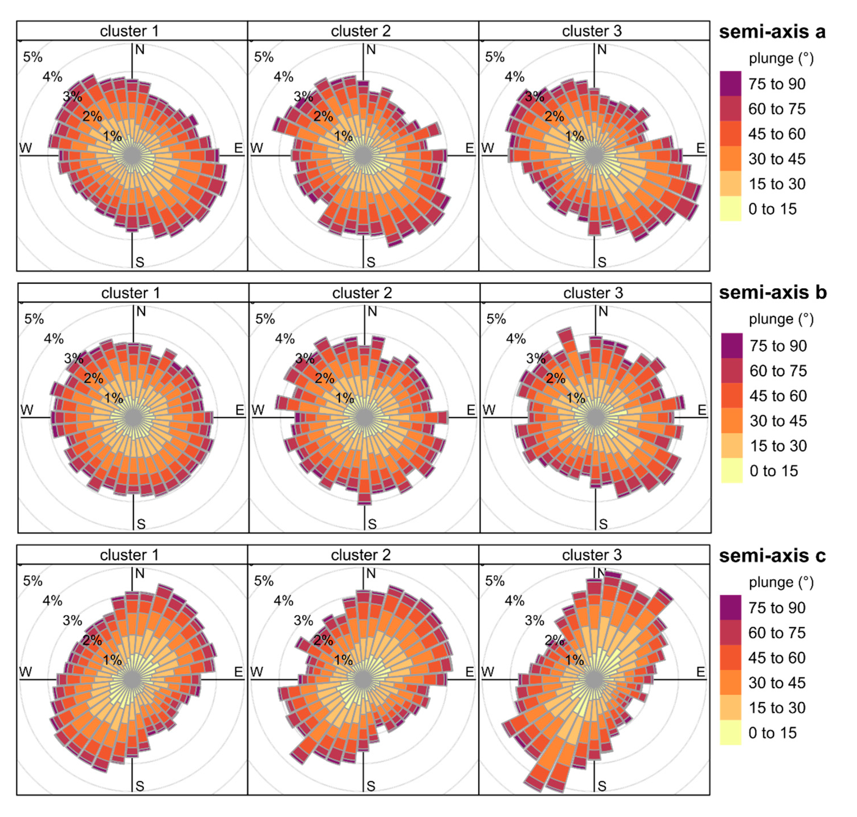
| 18 | semi-axis a | the length of the longest semi-axis of the ellipsoid | |
| 19 | semi-axis b | the length of the intermediate semi-axis of the ellipsoid | |
| 20 | semi-axis c | the length of the shortest semi-axis of the ellipsoid | |
| 21 | mean radius | mean distance from the geometrical centre of the object to the surface | |
| 22 | radius SD | the standard deviation of distance from the geometrical centre of the object to surface | |
| 23 | max radius | maximum distance from the geometrical centre of the object to the surface | |
| 24 | min radius | minimum distance from the geometrical centre of the object to the surface | |
| Shape | 25 | compactness | the normalized ratio between the surface and the volume of the object |
| 26 | discrete compactness | the measure of compactness for porous and fragmented objects basing on the face-connectivity of voxels within the object | |
| 27 | sphericity | root square of the compactness | |
| 28 | Euler number | the number of connected fragments of the object, minus the number of holes in the object, plus the number of bubbles within it | |
| 29 | geodesic elongation | the ratio between the geodesic diameter and the diameter of the largest inscribed ball | |
| 30 | semi-axes ratio a/b | the ratio between the length of the largest and medium semi-axis of the ellipsoid | |
| 31 | semi-axes ratio a/c | the ratio between the lengths of the largest and smallest semi-axis of the ellipsoid | |
| 32 | semi-axes ratio b/c | the ratio between the length of the medium and smallest semi-axis of the ellipsoid | |
| 33 | object vol./ellipsoid vol. ratio | the ratio between the volume of the object and the ellipsoid | |
| 34 | object vol./box vol. ratio | the ratio between the volume of the object and the bounding box | |
| 35 | ball vol./object vol. ratio | the ratio between the volume of the ball and the object | |
| Spatial Arrangement and Orientation | 36 | x coordinate | x coordinate of the geometrical centre for each object |
| 37 | y coordinate | y coordinate of the geometrical centre for each object | |
| 38 | z coordinate | z coordinate of the geometrical centre for each object | |
| 39 | semi-axis a trend | the direction of the ellipsoid’s semi-axis a on the xy plane measured clockwise from the north | |
| 40 | semi-axis a plunge | the vertical angle, measured downwards, between the xy plane and the ellipsoid’s semi-axis a | |
| 41 | semi-axis b trend | the direction of the ellipsoid’s semi-axis b on the xy plane measured clockwise from the north | |
| 42 | semi-axis b plunge | the vertical angle, measured downwards, between the xy plane and the ellipsoid’s semi-axis b | |
| 43 | semi-axis c trend | the direction of the ellipsoid’s semi-axis c on the xy plane measured clockwise from the north | |
| 44 | semi-axis c plunge | the vertical angle, measured downwards, between the xy plane and the ellipsoid’s semi-axis c |
| Library Name and Version | Usage | Reference |
|---|---|---|
| base_4.0.3 | data manipulation | [47] |
| openair_2.8-1 | data visualization | [48] |
| ggpmisc_0.3.7 | data manipulation | [49] |
| cluster_2.1.0 | cluster analysis | [50] |
| viridis_0.5.1 | data visualization | [51] |
| Morpho_2.8 | data manipulation | [52] |
| ggrepel_0.9.0 | data visualization | [53] |
| gridExtra_2.3 | data visualization | [54] |
| tidyverse_1.3.0 | data manipulation | [55] |
| reshape2_1.4.4 | data manipulation | [56] |
| factoextra_1.0.7 | cluster analysis | [57] |
| qgraph_1.6.5 | data visualization | [58] |
| ggplot2_3.3.3 | data visualization | [59] |
| corrplot_0.84 | data visualization | [60] |
| psych_2.0.12 | data exploration | [61] |
| DescTools_0.99.39 | data manipulation | [62] |
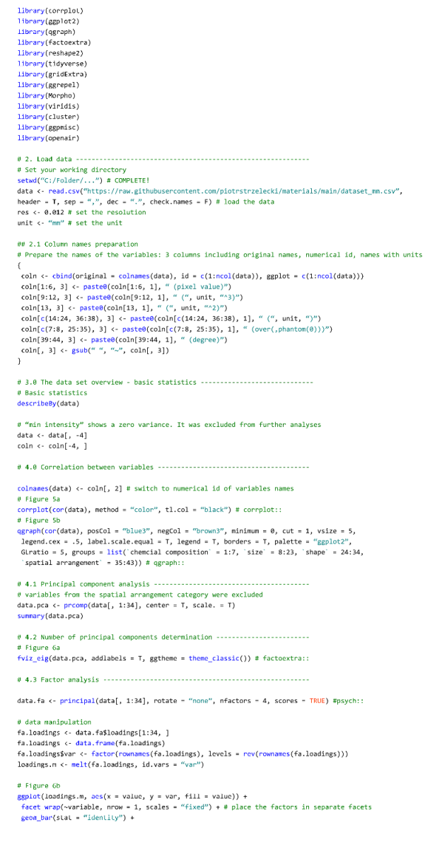
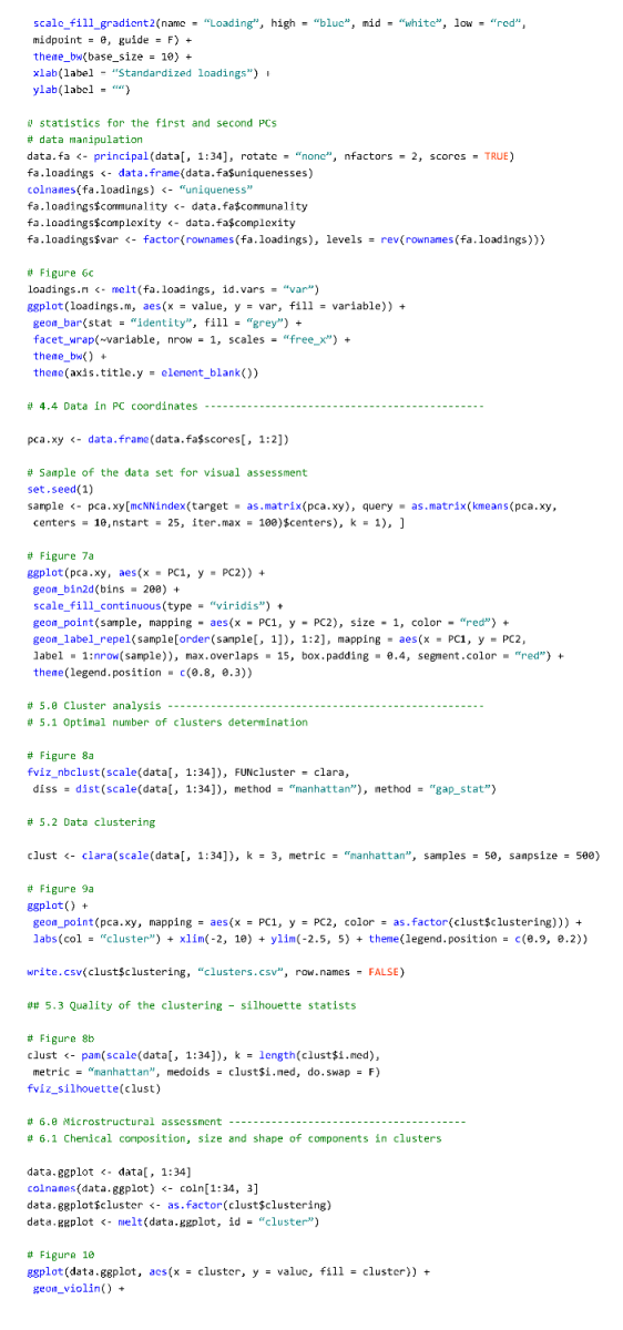
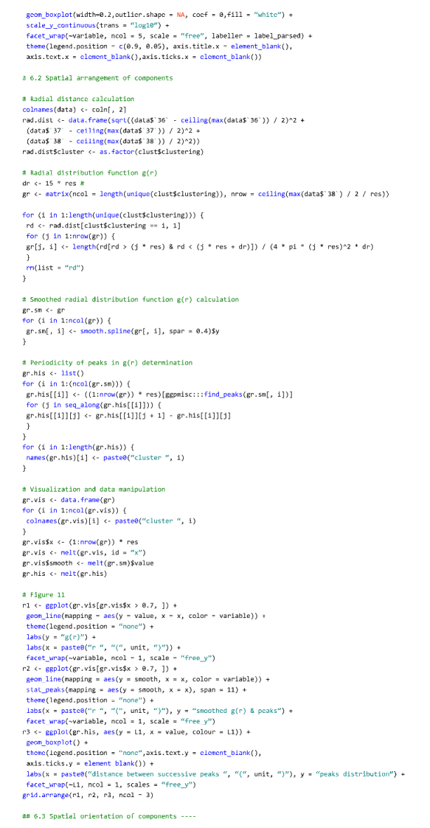
Appendix D. The Code for Data Set Analysis
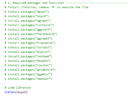

Appendix E. The Protocol Validation on a Standard Sample
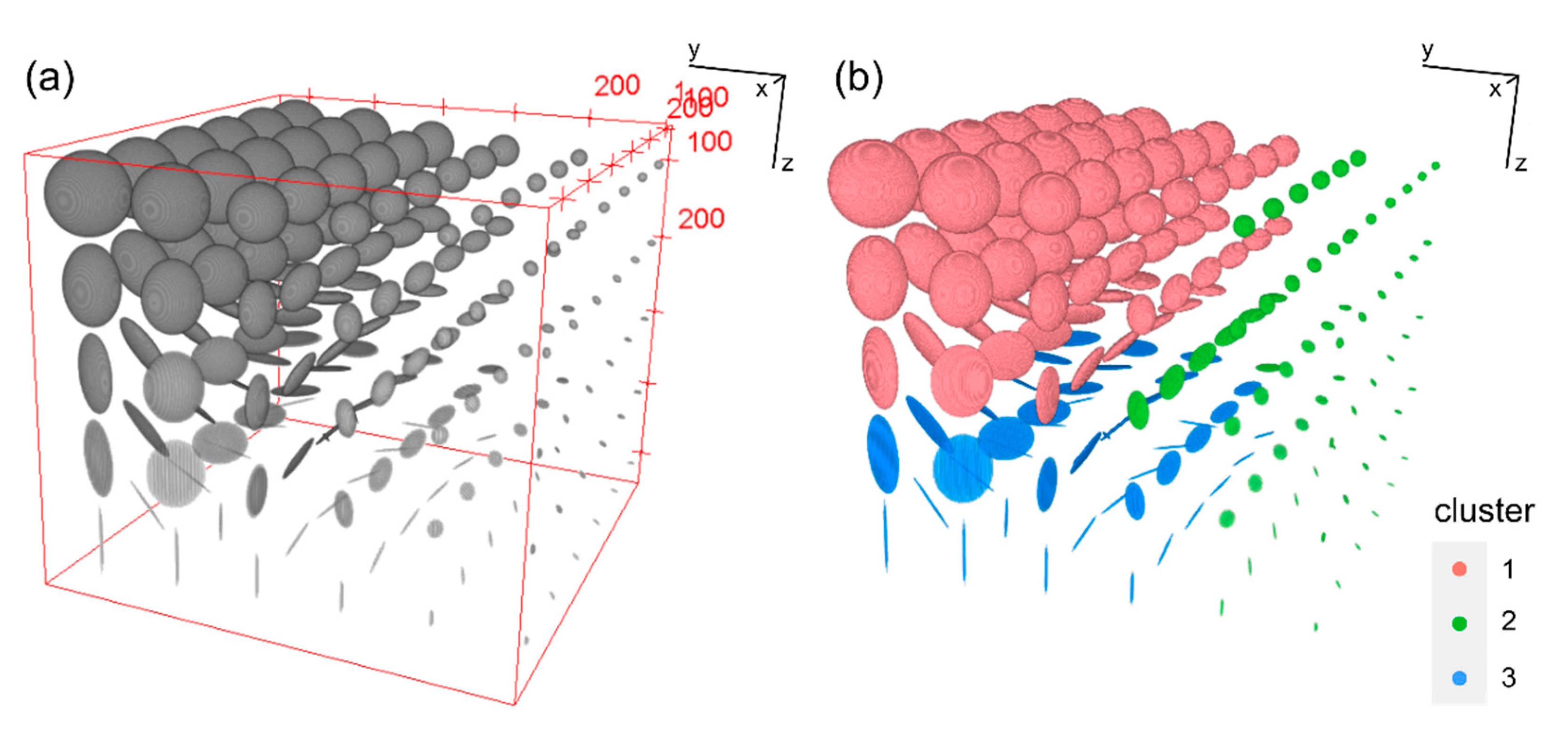
References
- Lindqvist, J.E.; Åkesson, U.; Malaga, K. Microstructure and functional properties of rock materials. Mater. Charact. 2007, 58, 1183–1188. [Google Scholar] [CrossRef]
- Strzelecki, P.J.; Fheed, A.; Radzik, N.; Świerczewska, A. X-ray microtomography and digital image analysis application to a petrological characterization of carbonates. Przegląd Geol. 2019, 67, 195–197. [Google Scholar] [CrossRef]
- Promentilla, M.A.B.; Cortez, S.M.; Papel, R.A.D.C.; Tablada, B.M.; Sugiyama, T. Evaluation of microstructure and transport properties of deteriorated cementitious materials from their X-ray computed tomography (CT) images. Materials 2016, 9, 388. [Google Scholar] [CrossRef]
- Rajczakowska, M.; Stefaniuk, D.; Łydżba, D. Microstructure Characterization by Means of X-ray Micro-CT and Nanoindentation Measurements. Studia Geotech. Mech. 2015, 37, 75–84. [Google Scholar] [CrossRef]
- Schmith, J.; Höskuldsson, Á.; Holm, P.M. Grain shape of basaltic ash populations: Implications for fragmentation. Bull. Volcanol. 2017, 79. [Google Scholar] [CrossRef]
- Bishwal, R.M. Potential use of R-statistical programming in the field of geoscience. In Proceedings of the 2017 2nd International Conference for Convergence in Technology (I2CT), Mumbai, India, 7–9 April 2017; IEEE: New York, NY, USA, 2017; pp. 979–982. [Google Scholar] [CrossRef]
- Rabbani, A.; Jamshidi, S.; Salehi, S. An automated simple algorithm for realistic pore network extraction from micro-tomography images. J. Pet. Sci. Eng. 2014, 123, 164–171. [Google Scholar] [CrossRef]
- Strzelecki, P.J.; Fheed, A.; Raczyński, P. 3D geometric evaluation of porosity types in carbonates. In AIP Conference Proceedings; AIP Publishing LLC: Melville, NY, USA, 2020; p. 030002. [Google Scholar] [CrossRef]
- Cheng, G.; Yue, Q. Rock Images Analysis of FCM Clustering Algorithm Based on Weighted Color Texture Features. J. Phys. Conf. Ser. 2018, 1, 012185. [Google Scholar] [CrossRef]
- Lai, J.; Lortie, C.J.; Muenchen, R.A.; Yang, J.; Ma, K. Evaluating the popularity of R in ecology. Ecosphere 2019, 10, e02567. [Google Scholar] [CrossRef]
- Royo, H. Programming Tools: Adventures with R. Nature 2015, 517, 109–110. [Google Scholar]
- Hydzik-Wiśniewska, J.; Pękala, A. The evaluation of the physico-mechanical properties of selected carpathian sandstones in terms of their use as a armourstone. Arch. Min. Sci. 2019, 64, 65–77. [Google Scholar] [CrossRef]
- Karnkowski, P. Oil and Gas Deposits in Poland; Geosynoptics Society: Cracow, Poland, 1999. [Google Scholar]
- Hurai, V.; Marko, F.; Tokarski, A.K.; Świerczewska, A.; Kotulová, J.; Biroň, A. Fluid inclusion evidence for deep burial of the Tertiary accretionary wedge of the Carpathians. Terra Nova 2006, 18, 440–446. [Google Scholar] [CrossRef]
- Pszonka, J.; Wendorff, M. Carbonate cements and grains in submarine fan sandstones—The Cergowa Beds (Oligocene, Carpathians of Poland) recorded by cathodoluminescence. Int. J. Earth Sci. 2017, 106, 269–282. [Google Scholar] [CrossRef]
- Jarmołowicz-Szulc, K.; Karwowski, Ł.; Marynowski, L. Fluid circulation and formation of minerals and bitumens in the sedimentary rocks of the Outer Carpathians—Based on studies on the quartz-calcite-organic matter association. Mar. Pet. Geol. 2012, 32, 138–158. [Google Scholar] [CrossRef]
- Świerczewska, A.; Tokarski, A.K. Deformation bands and the history of folding in the Magura nappe, Western Outer Carpathians (Poland). Tectonophysics 1998, 297, 73–90. [Google Scholar] [CrossRef]
- Strzelecki, P.J.; Tokarski, A.K.; Świerczewska, A. Structural evolution of the eastern part of the Silesian Nappe recorded in deformation bands, Polish segment of the Outer Carpathians. In Proceedings of the 16th Meeting of the Central European Tectonic Groups, Rytro, Poland, 18–21 April 2018; Tomaszczyk, M., Głuszyński, A., Sikora, R., Eds.; AGH University of Science and Technology: Cracow, Poland, 2018; Volume 44, p. 196. [Google Scholar] [CrossRef]
- Feldkamp, L.A.; Davis, L.C.; Kress, J.W. Practical cone-beam algorithm. J. Opt. Soc. Am. A 1984, 1, 612. [Google Scholar] [CrossRef]
- Bam, L.C.; Miller, J.A.; Becker, M. A mineral X-ray linear attenuation coefficient tool (MXLAC) to assess mineralogical differentiation for X-ray computed tomography scanning. Minerals 2020, 10, 441. [Google Scholar] [CrossRef]
- Guntoro, P.I.; Ghorbani, Y.; Koch, P.H.; Rosenkranz, J. X-ray microcomputed tomography (µct) for mineral characterization: A review of data analysis methods. Minerals 2019, 9, 183. [Google Scholar] [CrossRef]
- Schindelin, J.; Arganda-Carreras, I.; Frise, E.; Kaynig, V.; Longair, M.; Pietzsch, T.; Preibisch, S.; Rueden, C.; Saalfeld, S.; Schmid, B.; et al. Fiji: An open-source platform for biological-image analysis. Nat. Methods 2012, 9, 676–682. [Google Scholar] [CrossRef]
- Peng, T.; Thorn, K.; Schroeder, T.; Wang, L.; Theis, F.J.; Marr, C.; Navab, N. A BaSiC tool for background and shading correction of optical microscopy images. Nat. Commun. 2017, 8, 83–142. [Google Scholar] [CrossRef] [PubMed]
- Iassonov, P.; Gebrenegus, T.; Tuller, M. Segmentation of X-ray computed tomography images of porous materials: A crucial step for characterization and quantitative analysis of pore structures. Water Resour. Res. 2009, 45, 1–12. [Google Scholar] [CrossRef]
- Ollion, J.; Cochennec, J.; Loll, F.; Escudé, C.; Boudier, T. TANGO: A generic tool for high-throughput 3D image analysis for studying nuclear organization. Bioinformatics 2013, 29, 1840–1841. [Google Scholar] [CrossRef] [PubMed]
- Legland, D.; Arganda-Carreras, I.; Andrey, P. MorphoLibJ: Integrated library and plugins for mathematical morphology with ImageJ. Bioinformatics 2016, 32, 3532–3534. [Google Scholar] [CrossRef] [PubMed]
- Pearson, K. LIII. On lines and planes of closest fit to systems of points in space. Lond. Edinb. Dublin Philos. Mag. J. Sci. 1901, 2, 559–572. [Google Scholar] [CrossRef]
- Hotelling, H. Analysis of a complex of statistical variables into Principal Components. J. Educ. Psychol. 1933, 24, 417. [Google Scholar] [CrossRef]
- Abdi, H.; Williams, L.J. Principal component analysis. Wiley Interdiscip. Rev. Comput. Stat. 2010, 2, 433–459. [Google Scholar] [CrossRef]
- Spearman, C. ‘General Intelligence’, Objectively Determined and Measured. Am. J. Psychol. 1904, 15, 201–292. [Google Scholar] [CrossRef]
- Cattell, R. The Scree Test for the number of factors. Multivar. Behav. Res. 1966, 1, 245–276. [Google Scholar] [CrossRef]
- Hofmann, R.J. Indices Descriptive of Factor Complexity. J. Gen. Psychol. 1977, 96, 103–110. [Google Scholar] [CrossRef]
- Kaufman, L.; Rousseeuw, P.J. Clustering Large Data Sets; Elsevier Science Publishers B.V.: Amsterdam, The Netherlands, 1986. [Google Scholar]
- Kaufman, L.; Rousseuw, P.J. Finding Groups in Data: An Introduction to Cluster Analysis; John Wiley & Sons, Inc.: Hoboken, NJ, USA, 1990; ISBN 3175723993. [Google Scholar]
- Rousseeuw, P.J. Silhouettes: A graphical aid to the interpretation and validation of cluster analysis. J. Comput. Appl. Math. 1987, 20, 53–65. [Google Scholar] [CrossRef]
- Hintze, J.L.; Nelson, R.D. Violin plots: A box plot-density trace synergism. Am. Stat. 1998, 52, 181–184. [Google Scholar] [CrossRef]
- Scott, G.D. Radial Distribution of the Random Close Packing of Equal Spheres. Nature 1962, 194, 956–957. [Google Scholar] [CrossRef]
- Hair, J.F.; Black, W.C.; Babin, B.; Anderson, R.E. Multivariate Data Analysis, 7th ed.; Pearson: New York, NY, USA, 2010; ISBN 9780138132637. [Google Scholar]
- Arora, P.; Deepali; Varshney, S. Analysis of K-Means and K-Medoids Algorithm for Big Data. Phys. Procedia 2016, 78, 507–512. [Google Scholar] [CrossRef]
- Aggarwal, C.C.; Hinneburg, A.; Keim, D.A. On the surprising behavior of distance metrics in high dimensional space. In Proceedings of the International Conference on Database Theory, London, UK, 4–6 January 2001; Springer: Berlin/Heidelberg, Germany, 2001; Volume 1973, pp. 420–434. [Google Scholar] [CrossRef]
- Charrad, M.; Ghazzali, N.; Boiteau, V.; Niknafs, A. Nbclust: An R package for determining the relevant number of clusters in a data set. J. Stat. Softw. 2014, 61, 1–36. [Google Scholar] [CrossRef]
- Theodoridis, S.; Koutroumbas, K. Pattern Recognition, 4th ed.; Academic Press: Cambridge, MA, USA, 2008; ISBN 9781597492720. [Google Scholar]
- Pettijohn, F.J.; Potter, P.E.; Siever, R. Sand and Sandstone; Springer: New York, NY, USA, 1987; ISBN 978-0-387-96350-1. [Google Scholar]
- Stachowska, A.; Łoziński, M.; Śmigielski, M.; Wysocka, A.; Jankowski, L.; Ziółkowski, P. Anisotropy of magnetic susceptibility as an indicator for palaeocurrent analysis in folded turbidites (Outer Western Carpathians, Poland). Sedimentology 2020, 67, 3783–3808. [Google Scholar] [CrossRef]
- Legland, D.; Arganda-Carreras, I. MorphoLib User Manual. 2018. Available online: https://github.com/ijpb/MorphoLibJ/releases/download/v1.4.0/MorphoLibJ-manual-v1.4.0.pdf (accessed on 15 January 2021).
- Cordelieres, F.P. The 3D Object Counter Plugin a.k.a 3D-OC. 2009. Available online: https://imagejdocu.tudor.lu/_media/plugin/analysis/3d_object_counter/3d-oc.pdf (accessed on 15 January 2021).
- R Core Team. R: A Language and Environment for Statistical Computing; R Foundation for Statistical Computing: Vienna, Austria, 2020. [Google Scholar]
- Carslaw, D.C.; Ropkins, K. Openair—An r package for air quality data analysis. Environ. Model. Softw. 2012, 27, 52–61. [Google Scholar] [CrossRef]
- Aphalo, P.J. Ggpmisc: Miscellaneous Extensions to ‘Ggplot2’; R Package Version 0.3.7; R Foundation for Statistical Computing: Vienna, Austria, 2020. [Google Scholar]
- Maechler, M.; Rousseeuw, P.; Struyf, A.; Hubert, M.; Hornik, K. Cluster: Cluster Analysis Basics and Extensions, R package version 2.1.0; R Foundation for Statistical Computing: Vienna, Austria, 2019. [Google Scholar]
- Garnier, S. Viridis: Default Color Maps from ‘Matplotlib; R Package Version 0.5.1; R Foundation for Statistical Computing: Vienna, Austria, 2018. [Google Scholar]
- Schlager, S. Morpho and Rvcg—Shape Analysis in {R}. In Statistical Shape and Deformation Analysis; Zheng, G., Li, S., Szekel, G., Eds.; Academic Press: Cambridge, MA, USA, 2017; pp. 217–256. ISBN 9780128104934. [Google Scholar]
- Słowikowski, K. Ggrepel: Automatically Position Non-Overlapping Text Labels with ‘ggplot2’; R Package Version 0.9.0; R Foundation for Statistical Computing: Vienna, Austria, 2020. [Google Scholar]
- Auguie, B. Gridextra: Miscellaneous Functions for ‘Grid’ Graphics; R Package Version 2.3; R Foundation for Statistical Computing: Vienna, Austria, 2017. [Google Scholar]
- Wickham, H.; Averick, M.; Bryan, J.; Chang, W.; McGowan, L.; François, R.; Grolemund, G.; Hayes, A.; Henry, L.; Hester, J.; et al. Welcome to the Tidyverse. J. Open Source Softw. 2019, 4, 1686. [Google Scholar] [CrossRef]
- Wickham, H. Reshaping Data with the reshape Package. J. Stat. Softw. 2007, 21, 1–20. [Google Scholar] [CrossRef]
- Kassambara, A.; Mundt, F. Factoextra: Extract and Visualize the Results of Multivariate Data Analyses; R Package Version 1.0.7; R Foundation for Statistical Computing: Vienna, Austria, 2020. [Google Scholar]
- Epskamp, S.; Cramer, A.O.J.; Waldorp, L.J.; Schmittmann, V.D.; Borsboom, D. Qgraph: Network visualizations of relationships in psychometric data. J. Stat. Softw. 2012, 48. [Google Scholar] [CrossRef]
- Wickham, H. Ggplot2: Elegant Graphics for Data Analysis; Springer: New York, NY, USA, 2016. [Google Scholar]
- Wei, T.; Simko, V. R Package ‘Corrplot’: Visualization of a Correlation Matrix; R Package Version 0.84; R Foundation for Statistical Computing: Vienna, Austria, 2017. [Google Scholar]
- Revelle, W. Psych: Procedures for Psychological, Psychometric, and Personality Research; R Package Version 2.0.12; R Foundation for Statistical Computing: Vienna, Austria, 2020. [Google Scholar]
- Andri, S.; Aho, K.; Alfons, A.; Anderegg, N.; Aragon, T.; Arachchige, C.; Arppe, A.; Baddeley, A.; Barton, K.; Bolker, B.; et al. DescTools: Tools for Descriptive Statistics; R Package Version 0.99.39; R Foundation for Statistical Computing: Vienna, Austria, 2020. [Google Scholar]

Publisher’s Note: MDPI stays neutral with regard to jurisdictional claims in published maps and institutional affiliations. |
© 2021 by the authors. Licensee MDPI, Basel, Switzerland. This article is an open access article distributed under the terms and conditions of the Creative Commons Attribution (CC BY) license (https://creativecommons.org/licenses/by/4.0/).
Share and Cite
Strzelecki, P.J.; Świerczewska, A.; Kopczewska, K.; Fheed, A.; Tarasiuk, J.; Wroński, S. Decoding Rocks: An Assessment of Geomaterial Microstructure Using X-ray Microtomography, Image Analysis and Multivariate Statistics. Materials 2021, 14, 3266. https://doi.org/10.3390/ma14123266
Strzelecki PJ, Świerczewska A, Kopczewska K, Fheed A, Tarasiuk J, Wroński S. Decoding Rocks: An Assessment of Geomaterial Microstructure Using X-ray Microtomography, Image Analysis and Multivariate Statistics. Materials. 2021; 14(12):3266. https://doi.org/10.3390/ma14123266
Chicago/Turabian StyleStrzelecki, Piotr Jan, Anna Świerczewska, Katarzyna Kopczewska, Adam Fheed, Jacek Tarasiuk, and Sebastian Wroński. 2021. "Decoding Rocks: An Assessment of Geomaterial Microstructure Using X-ray Microtomography, Image Analysis and Multivariate Statistics" Materials 14, no. 12: 3266. https://doi.org/10.3390/ma14123266
APA StyleStrzelecki, P. J., Świerczewska, A., Kopczewska, K., Fheed, A., Tarasiuk, J., & Wroński, S. (2021). Decoding Rocks: An Assessment of Geomaterial Microstructure Using X-ray Microtomography, Image Analysis and Multivariate Statistics. Materials, 14(12), 3266. https://doi.org/10.3390/ma14123266


