Article

Characterization and Simulation of the Bond Response of NSM FRP Reinforcement in Concrete

AMADE, Polytechnic School, University of Girona, 17003 Girona, Spain
*
Author to whom correspondence should be addressed.
Materials 2020, 13(7), 1770; https://doi.org/10.3390/ma13071770
Submission received: 6 February 2020 / Revised: 29 March 2020 / Accepted: 7 April 2020 / Published: 9 April 2020

Abstract

:
The near-surface mounted (NSM) technique with fiber reinforced polymer (FRP) reinforcement as strengthening system for concrete structures has been broadly studied during the last years. The efficiency of the NSM FRP-to-concrete joint highly depends on the bond between both materials, which is characterized by a local bond–slip law. This paper studies the effect of the shape of the local bond–slip law and its parameters on the global response of the NSM FRP joint in terms of load capacity, effective bond length, slip, shear stress, and strain distribution along the bonded length, which are essential parameters on the strengthening design. A numerical procedure based on the finite difference method to solve the governing equations of the FRP-to-concrete joint is developed. Pull-out single shear specimens are tested in order to experimentally validate the numerical results. Finally, a parametric study is performed. The effect of the bond–shear strength slip at the bond strength, maximum slip, and friction branch on the parameters previously described is presented and discussed.

1. Introduction

The use of fiber reinforced polymer (FRP) materials for strengthening existing concrete structures has been widely studied during the last years because of the potential advantages of these materials compared to the conventional ones [1]. The most commonly used techniques for strengthening reinforced concrete (RC) structures with FRPs are the so-called externally bonded reinforcement (EBR) and near-surface mounted (NSM) reinforcement. While in the EBR methodology the FRP reinforcement is bonded on the exterior face of the structural element, in the NSM system the FRP is installed into groves cut in the concrete cover where it is bonded with the appropriate adhesive. The NSM technique has attracted the attention of researchers and industry in recent years due to several potential advantages compared to the EBR system, such as no need of specific surface preparation except grooving, better anchorage capacity, better protection in front of external agents like fire or vandalism, and no relevant change in the aesthetics of the structural element [2].
A number of research works have been carried out in order to obtain analytical solutions of the differential equations governing the bond performance of the FRP-to-concrete joint. This differential equation is based on the local bond–slip behavior, relating the bond and slip at every point along the bonded length. For the EBR technique, for instance, Yuan et al. proposed an analytical solution based on a local bilinear bond–slip law in [3] and a trilinear bond–slip one with an exponential descending branch in [4]. In a later work, Ali et al. [5] adapted Yuan’s analytical solution to the NSM strengthening system. Even though these authors proposed closed form equations to calculate the global bond behavior, these are not always easy to implement and are only suitable for specific local bond–slip laws.
In recent years, experimental and numerical studies have provided solutions to the global bond behavior of the EBR strengthening technique [6,7,8,9,10,11,12], although less attention has been paid to the NSM strengthening systems [13,14]. Focusing specifically on the characterization of the local bond behavior of NSM FRP-to-concrete joints, several bond–slip laws have been proposed in the literature, with different shapes and stages. Some examples are the models proposed by Sena et al. [13], Borchert et al. [14], Zhang et al. [15], and Seracino et al. [16]. The effect of their differences on the structural bond response and design implications is not always straightforward, thus, development of numerical tools that allow obtaining and comparing the response for different models is of main interest.
The aim of this paper is to study the effect of the shape of the local bond–slip law on the global bond behavior of NSM FRP strengthening systems. For this purpose, a numerical procedure based on finite difference method is proposed to solve in a general way the differential equation that characterizes the bond behavior of the FRP-to-concrete joint, which can be applied independently of the specific local bond–slip law. The numerical results are then verified by comparison between numerical and experimental results. Finally, a parametric study to evaluate the effects of the parameters defining the local behavior of the NSM FRP strengthened bonded joint is carried out.

2. Bond Mechanisms in NSM FRP Strengthening Systems

In the NSM FRP strengthening system, the forces are transferred from the FRP material to the internal faces of the concrete groove through its perimeter in contact with the adhesive. This way, there are two main issues improving the transfer of stresses with respect to the EBR reinforcement: the higher ratio of the area of the perimeter in contact with the adhesive to the FRP area, and the transmission to the concrete material through a confined zone in the interior of the slot in the concrete cover.
The global bond stress-slip response for NSM strips subjected to a pull-out force is generally characterized by an initial, relatively stiff, linear behavior, followed by a nonlinear curve up to the maximum value of the bond stress (bond strength), after which the originated damage causes a softening branch. Moreover, in NSM strengthening systems, it has been observed the activation of a friction component for relatively large slips as an extension of the softening branch [1,14,17,18,19]. The presence of a friction branch has been also reported in the bond behavior of other strengthening materials as fiber reinforced cementitious matrix composites (FRCM) [20,21].
The bond mechanisms generated in the NSM FRP technique can lead to several types of failure modes, which are mainly influenced by the bonded length, FRP surface and shape, groove configuration, materials mechanical properties and adhesive properties [22,23]. In general, the failure modes can be grouped into three main categories: failure at the FRP-adhesive interface, failure at the epoxy–concrete interface, and adhesive cover splitting [1].
The global bond stress-slip performance of an NSM FRP strip bonded to a concrete block is the result of the local bond–slip behavior at every point along the bonded length, which can be considered the constitutive model characterizing the bond behavior of the NSM FRP element. Different models and shapes can be found in the literature for these local laws, and the assessment of their results is the main objective of this paper.

3. Assessment of the Bond–Slip Response of NSM FRP

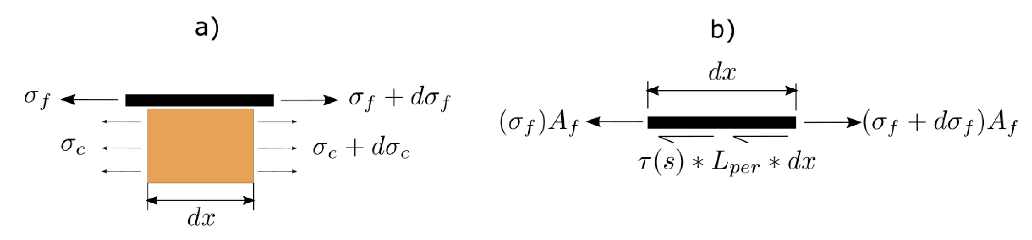
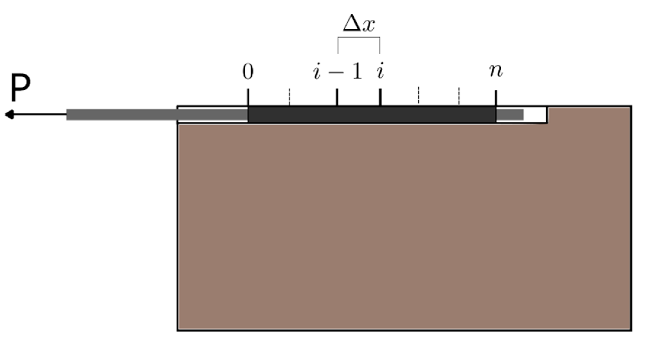
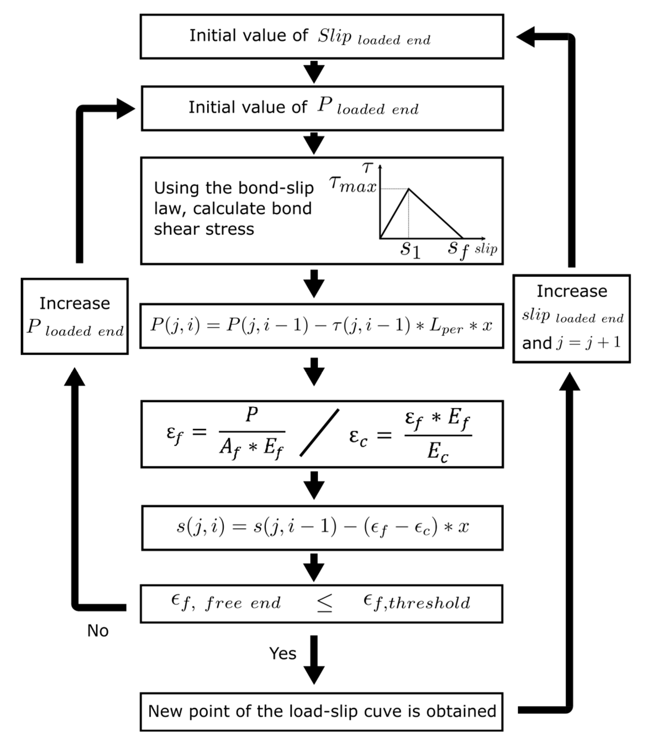
3.1. Governing Equation and Global Response

In the single shear pull-out test (pull-push test), the load is transferred from the FRP to the concrete through the adhesive. Figure 1a shows the stress equilibrium of an infinitesimal element of FRP NSM concrete element of length dx. Figure 1b shows the stress equilibrium of the FRP-adhesive interface in an infinitesimal element of length dx.
From stress equilibrium between FRP and concrete, and the FRP-adhesive interface, Equation (1) and Equation (2) can be obtained.
A f d σ f + A c d σ c = 0 ,
d σ f d x τ ( s ) * L p e r A f = 0 ,
where σf is the stress in the FRP, Af is the FRP area, calculated as the product of the FRP thickness (tf) by the FRP width (wf), σc is the stress in the concrete, Ac is the area of concrete, τ(s) is the bond–slip law of the joint, and Lper is the is the intermediate perimeter in the adhesive.
The slip of the bonded joint can be defined as the relative displacement between the FRP and the concrete element.
s = u f u c ,
where s is the slip, uf is the FRP displacement and uc is the concrete displacement. Using the constitutive equations of the FRP and the concrete, Equation (4) and Equation (5) are obtained.
d s d x = ε f ε c = σ f E f σ c E c ,
d 2 s d x 2 = 1 E f d σ f d x 1 E c d σ c d x ,
where Ef is the elastic modulus of the FRP, εf is the strain in the FRP, Ec is the elastic modulus of the concrete, and εc is the strain in the concrete.
Finally, by substituting Equation (1) and Equation (2) into Equation (5), the differential equation governing the bond–slip behavior of a NSM FRP-to–concrete bonded joint is:
d 2 s ( x ) d x 2 τ ( s ) * L p e r ( 1 E f * A f 1 E c * A c ) = 0 ,
It is worth mentioning that usually the second term in the parenthesis corresponding to the concrete properties is much lower than the first and can be neglected (Ko et al. [24]).
Equation (6) can be solved analytically using the boundary conditions
ε f = 0   at   x = 0 ,
s = s ( L b )   at   x = L b ,
where εf is the strain in the FRP at the free end, Lb is the bonded length, and s(Lb) is the applied slip at the loaded end.
This differential equation can be solved for specific shapes of the local bond-stress slip law [3]. In the rest of cases a numerical procedure is required.
The numerical model implemented in this work is based on the finite difference method and aims to solve the governing equation of the bonded joint for any type of local bond–slip law. Following this methodology, the bonded length (Lb) is discretized into n uniform small increments of length Δx = Lb/n. The increments are delimited by n+1 points, which position is defined by xi = i·Δx (i = 0,1, …n) (Figure 2). The procedure is based on an incremental slip methodology that pretends to simulate a usual experimental test under monotonic increase of the loaded end slip (this way, possible snap-back effect after maximum load is not reproduced in the simulations, Zou et al. [21]). Starting from the loaded end and moving towards the free end, the procedure calculates, for every studied point, the slip and the load transmitted between two adjacent sections. For a certain value of slip at the loaded end, an iterative process is carried out in which P(j,1) is a lower bound value of the initial load at the loaded end at iteration j. P(j,1) is used to calculate the corresponding strain in the FRP (εFRP), the strain in the concrete (εc), and the bond–shear stress (τ) using the bond–slip law at the loaded point. Still, at iteration j, the load at every point i, P(j,i), is calculated using Equation (9) along the FRP and towards the free end, by
P ( j , i ) = P ( j , i 1 ) τ ( j , i 1 ) * L p e r * Δ x ,
From the load profile obtained using Equation (9), the strain distribution in the concrete and the FRP can be obtained, and, subsequently, the slip profile along the FRP is calculated as
s ( j , i ) = s ( j , i 1 ) ( ε f ε c ) * Δ x ,
Increments of P at the loaded end are applied until convergence is attained, which happens when the εf at the free end is less than a prescribed tolerance, set to be a value close to zero. Once convergence is achieved, the corresponding load is registered and the process is repeated for a new value of slip at the loaded end, defined as s(j+1,1). At this point, the iterative procedure is again repeated. The procedure finishes when all the points of the load–slip curve are calculated. Figure 3 shows the flowchart of the numerical procedure.

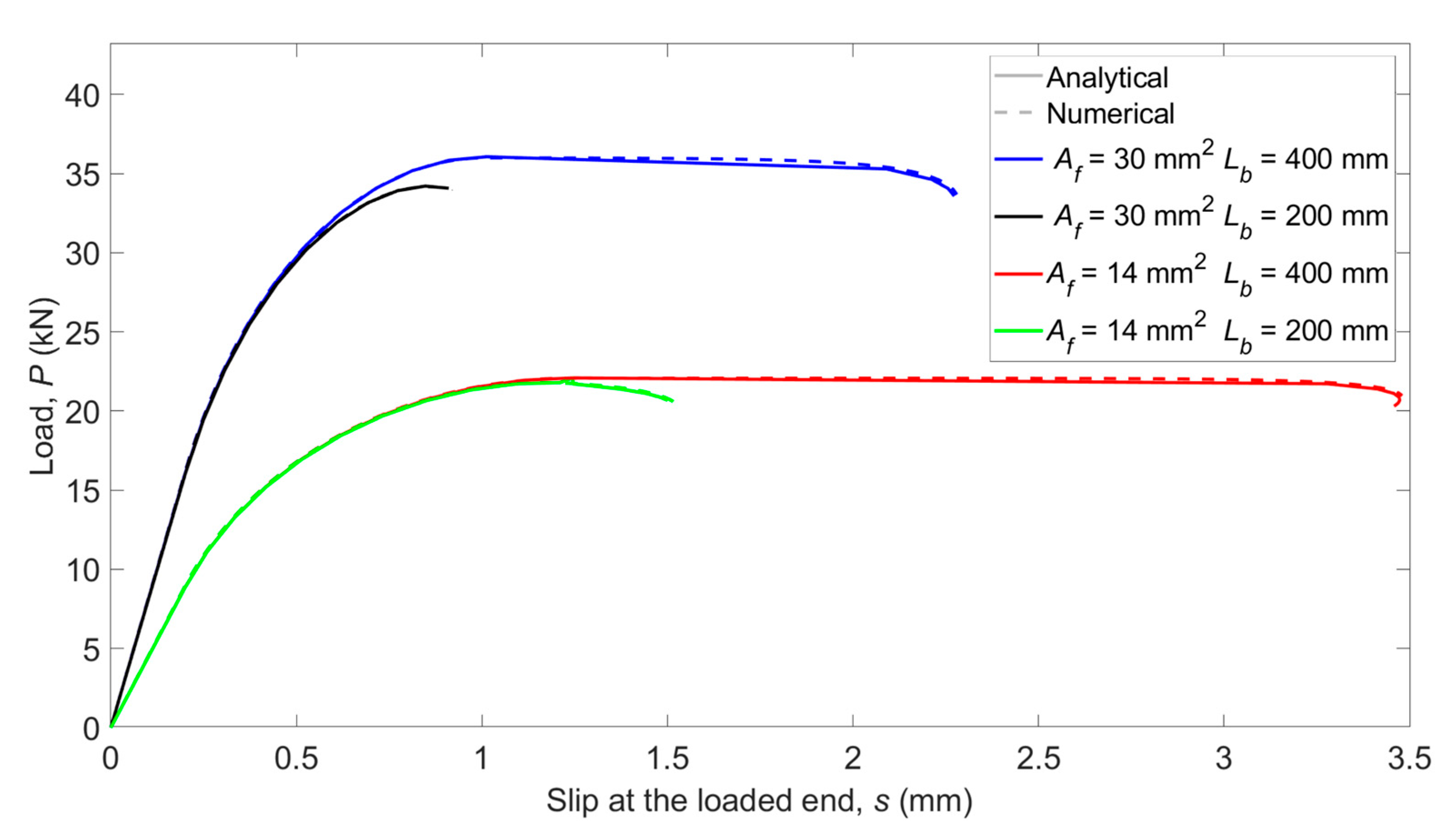
3.2. Comparison of the Numerical Results with Existing Analytical Solutions

In order to verify the numerical procedure developed, a comparison with analytical solutions available for some specific laws is presented in this section. For the sake of simplicity, only the analytical solution for the bilinear bond–slip law proposed by Yuan et al. [3] is taken as a reference, considering a bond–shear strength (τmax) of 15 MPa, a slip at the bond–shear strength (s1) of 0.1 mm and a maximum slip (sf) of 1.13 mm. These values have been chosen according to experimental results available in the literature. Four different situations are simulated by modifying the bonded length (Lb = 200 and 400 mm) and the FRP area (Af = 14 and 30 mm2). The results, presented in Figure 4, show good agreement between the analytical and the numerical solutions, and therefore the suitability of the developed procedure.

4. Bond–Slip Behavior at a Local Level

In this work, six different models (Table 1) based on two of the most widely accepted constitutive laws for bond characterization of NSM FRP systems (the Bilinear law [16] and Borchert law [14]) are considered. The study focuses on the effect of the combination of their parameters on the structural global response of the bonded joint. From the bilinear law, four combinations are studied: i) a bilinear (BL) model; ii) a linear descending (LD) model, which does not consider the initial elastic branch; iii) a two stage bond–slip law with a non-linear ascending branch (TSANL) model, with the aim to study the effect of the shape of the ascending branch; and iv) a bilinear plus friction (BLF) model, with the purpose to obtain the effect of friction in a bilinear bond–slip law. On the other hand, from Borchert law (BO), one additional modification is proposed, consisting in suppressing the original bond–shear strength plateau (BONP).

5. Global Bond–Slip Response for Different Local Bond–Slip Laws

The main objective of this section is to evaluate the influence of the local bond law on the global behavior of the FRP laminates bonded to concrete as NSM strengthening system, when subject to a pull-out force, using the numerical model described in Section 3, and the bond–slip laws introduced in Section 2.

5.1. Parameters Used

The values of the parameters that define the different local bond–slip laws, as well as the properties of materials and characteristics of specimens have been chosen according to previous experimental campaigns found in the literature [13,14,15,16,25,26], with the aim to simulate conditions as realistically as possible.
The elastic modulus of the laminate and concrete are 150 GPa and 33 GPa, respectively. The concrete block cross-section is 200 × 200 mm and the groove thickness and width are 5 mm and 15 mm, respectively. The bonded length (Lb) has been set as 200 mm, and the laminate section is 1.4 × 10 mm.
Regarding the bond–slip parameters, bond–shear strength has been set as 15 MPa, and the corresponding slip as 0.1 mm. In bond–slip models that have a friction branch, τf has been defined as the 35% of τmax. The initial point of the plateau of BO model is s 1 = 0.8 · s 2 , and the experimental parameter α is 0.31 [14].
Another parameter that is crucial for the simulations is the fracture energy (Gf), typically defined as the area under the bond–slip law [6]. In those bond–slip laws with a friction branch, Gf is calculated according to Haskett et al. [27], as the area under the ascending and descending stages of the bond–slip law, without taking into account the friction stage, as illustrated in Figure 5. A value of 8.5 N/mm has been set for Gf in all the models [16,25,26].
The comparison between the studied bond–slip laws is shown in Figure 6. As indicated before, it can be observed that the bond–shear strength (τmax) is 15 MPa, and the corresponding slip (s1) is 0.1 mm, except for the LD model, which does not consider s1.

5.2. Load–Slip Response

The comparison of the load–slip curves obtained from each bond–slip law is shown in Figure 7. Overall, two main tendencies can be observed. The first one (Figure 7a), followed by LD, BL and TSANL models, achieve a maximum load, which remains constant as the slip in the loaded end increases until failure. This plateau is obtained because the maximum activated length is attained when the slip in the loaded point is equal to sf, meaning that this point does not carry load anymore (debonding). Therefore, the load capacity will remain constant and the slip will keep increasing until failure. In the second trend (Figure 7b), followed by BLF, BO, and BONP models, the load increases up to the maximum carrying capacity, where a sudden decrease takes place followed by a residual (friction) bond force. The difference between these two trends falls to the effect of the friction branch of the local bond–slip law after the loaded point reaches debonding.
Focusing on the initial part of the load–slip curve (interior plot in Figure 7a) it can be seen that the LD model shows the highest stiffness, because the ascending branch of the bond–slip law has an infinite stiffness. Besides, it can be observed that bond–slip models with a non-linear ascending branch (TSANL, BO, and BONP) exhibit a stiffer branch of the load–slip curve than BL and BLF models caused by the fact that for a fixed value of s1 the area under the ascending branch is greater in those cases with non-linear tendency.

5.3. FRP Strain, Bond–Shear Stress and Slip along the Bonded Length

Following the numerical procedure, the FRP strain, bond–shear stress and slip can also be obtained. Figure 8 shows the response along the bonded length for the different laws (loaded end at x = 0 mm, free end at x = 200 mm) evaluated at the situation of imminent failure (marked with a red dot in Figure 7). For 7.5 mm grooved specimens, the failure point was defined as the point before the load drops to 0, and for 10 mm grooved specimens, the failure was defined as the maximum load point.
From Figure 8a it can be observed that the shape of the bond–slip law has a small effect on the slip profile along the FRP. It can also be seen that BLF, BO and BONP exhibit slightly higher values for the slip at the loaded end. Furthermore, the slip at the free end equals to 0 for the LD model, contrarily to the rest of models, which show a small value of slip.
An evident difference between the models with and without friction can be observed in the bond stress distribution along the bonded length (Figure 8b). Models that include friction still transmit bond–shear stress after the softening stage, whilst the other models exhibit a completely damaged zone, where no load is transmitted. Hence, for friction bond–slip models, the increase of the area under the bond–shear stress profile allows the joint to carry more load even though the zone near the loaded end is damaged.
Figure 8c shows the FRP strain distribution. In models without friction, the strain profile stabilizes when the maximum load is attained. On the other hand, strain values in the FRP do not stabilize for BLF, BO, and BONP models, because of the load keeps increasing after the loaded end surpasses the softening stage.

6. Experimental Program

In this section, an experimental program is presented and the results, in terms of load–slip curves are discussed. Then, a relatively simple methodology to obtain the bond–slip law from the experimental load–slip curve is presented. Finally, the theoretical results obtained from the numerical procedure are compared to experimental values.

6.1. Material Properties

The concrete used in the experimental campaign has been characterized according to the UNE 12390-3 [28] and the ASTM C469 / C469M-10 standard [29]. From the characterization tests on 150 × 300 mm cylindrical specimens, a compressive strength of 36.9 MPa and an elastic modulus of 46.8 GPa were obtained.
Carbon-FRP (CFRP) strips with 3 × 10 mm cross-section were used in the experimental campaign. Their mechanical properties were tested according to ISO 527-5 [30], obtaining an elastic modulus of 169.3 GPa and a tensile strength of 3205.9 MPa.
The bi-component epoxy resin used in this program was tested according to the ISO 527-2 standard [31] after 12 days of curing under 20ºC and 55%RH, obtaining an elastic modulus of 10.7 GPa and a tensile strength of 27.9 MPa.

6.2. Experimental Details

6.2.1. Parameters of the Study
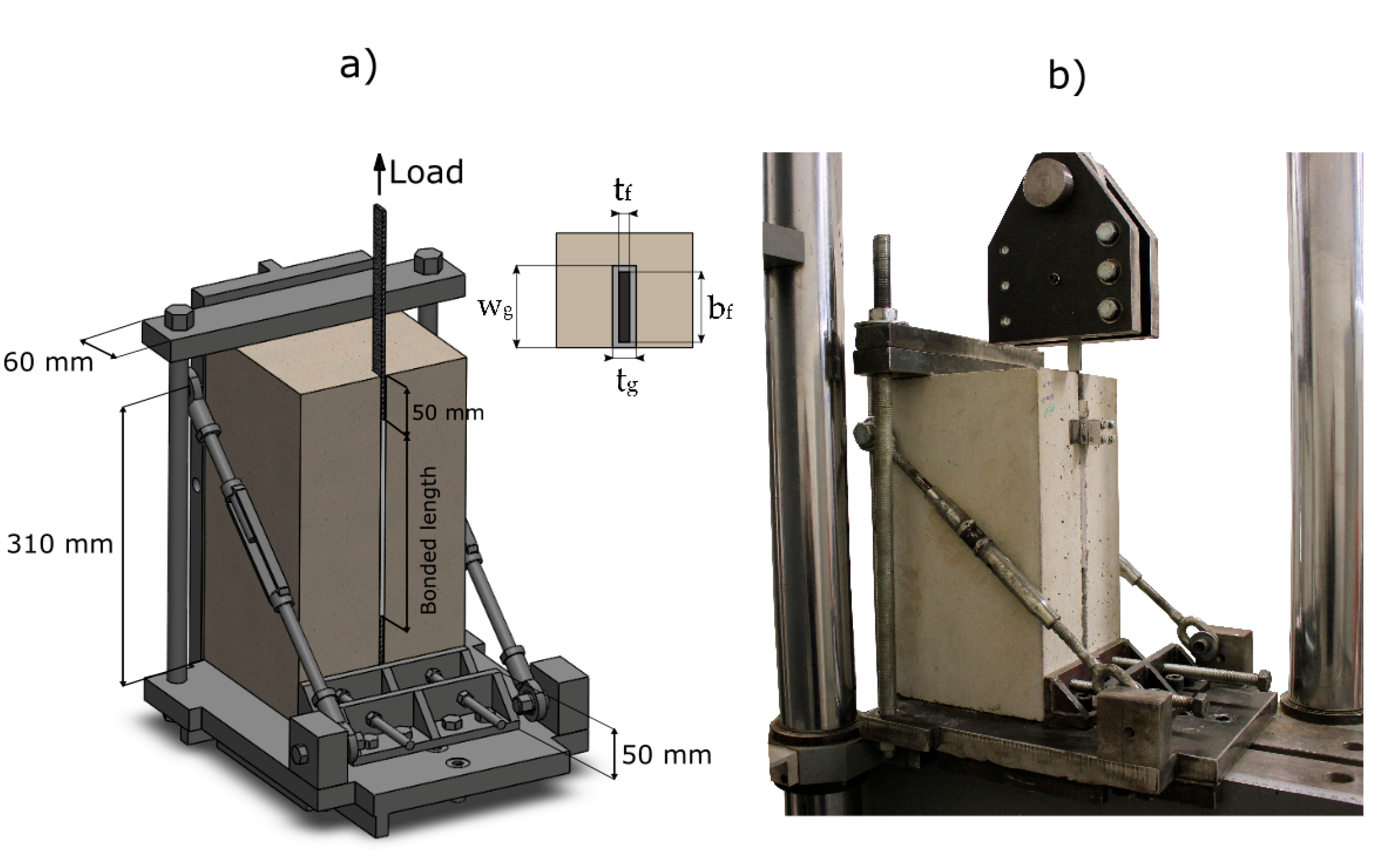
Four different NSM configurations were tested, combining two different groove thicknesses (7.5 mm and 10 mm) and two different bonded lengths (150 mm and 225 mm). Four specimens were tested per each configuration, giving a total of 16 specimens tested in a direct pull-out shear test.
The fib Bulletin 90 [1] limits the deepness of the groove in order to avoid epoxy cover splitting. ACI [32], in turn, suggests that the groove thickness should be, at least, 3 times the laminate thickness. In order to study the effect of the resin layer thickness, two groove thicknesses were defined in this study: 10 mm and 7.5 mm. The first one was set according to the ACI requirement, whilst the second groove thickness was chosen to satisfy the fib [1] condition that establishes that the minimum groove dimensions must be 1.5 or 2 times the laminate size.
Regarding the effect of the bonded length, Seracino et al. [33] used bonded lengths between 100 mm and 350 mm and concluded that the minimum Lb to achieve the maximum carrying capacity was 200 mm. Furthermore, Zhang et al. [34] tested NSM strengthened concrete elements with bonded lengths between 25 and 350 mm. From their study, it was observed that the experimental effective bonded lengths for the different specimens were between 150 and 175 mm.
The bonded lengths used in this experimental campaign were chosen to be above and below the values suggested in [33] and [34], in order to validate if the finite differences model is able to predict the response for short and long bonded lengths.

6.2.2. Test Setup

In order to study the effect of the bonded length and the groove width, four pull-out configurations were designed. Four specimens were tested for each configuration defined in Table 2.
The specimens were identified as NSM – Lbtg, where Lb stands for the bonded length and tg for the groove thickness. The tests were carried out under a single shear test configuration, as shown in Figure 9. The specimen was rigidly fixed with a 60 mm wide plate to avoid translation in the vertical direction and also perpendicularly in the opposite side with a 50 mm plate to avoid rotation. At the top of the specimen a length of 50 mm was left unbonded to avoid stress concentrations in that zone [35]. The concrete block dimensions used on the short-bonded length specimens were 200 × 200 × 370 mm, and for the long-bonded length specimens 200 × 200 × 420 mm. A servo-hydraulic testing machine was used to apply the load. The test was performed under displacement control with a speed of 0.2 mm/min. One LVDT was placed in the loaded end to measure the relative displacement between the CFRP strip and the concrete.

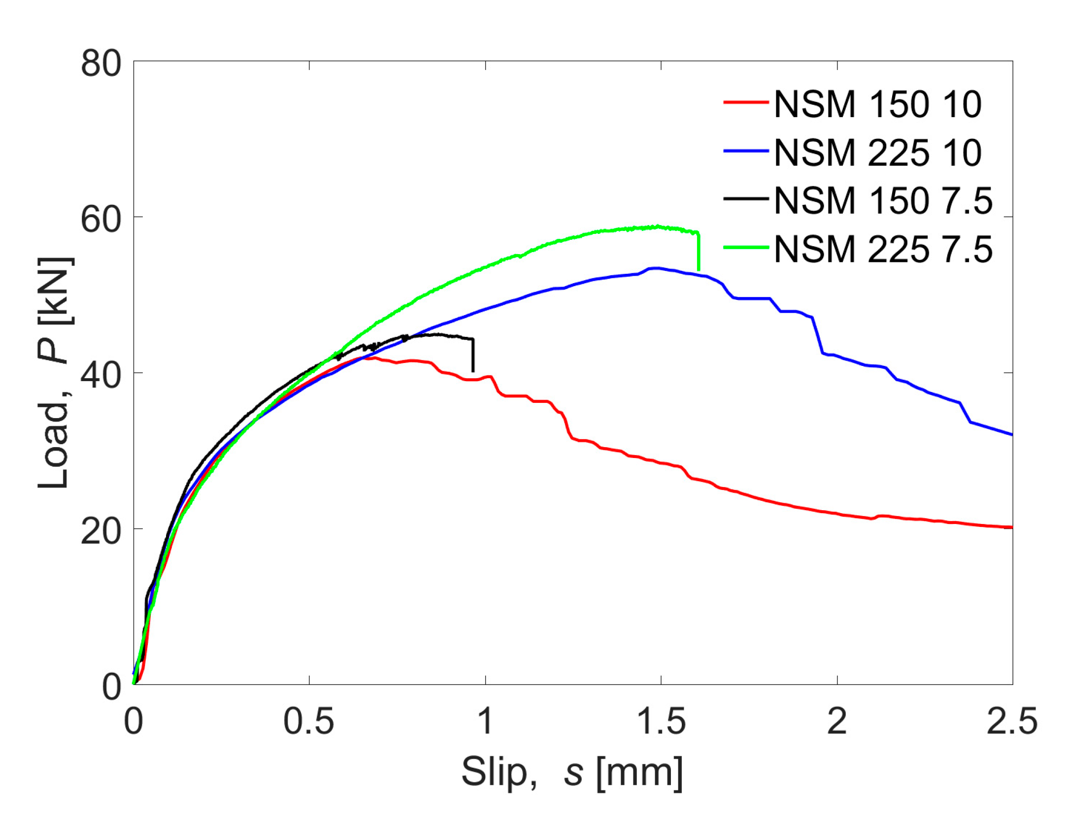
6.3. Experimental Results

The results obtained from the experimental tests are shown in Figure 10, where the average load–slip curves for the four tested configurations are presented.
Failure loads for the narrowest groove specimens were slightly higher than for those with the widest grooves: the failure load of NSM-150-7.5 was 7.1% higher than NSM-150-10, and NSM-225-7.5 failure load was 10.0% higher than in the NSM-225-10 case. Besides, differences in the failure load can be observed: 10 mm grove thickness specimens failed in the FRP-adhesive interface while 7.5 mm grove thickness specimens failed in the resin–concrete interface.
As can be observed, in specimens with 10 mm groove thickness, after reaching the maximum load, the slip continued increasing although the load decreased, which could be interpreted as all the bonded length being activated and damaged, as well as friction effect taking place. On the other hand, failure of the specimens with 7.5 mm groove was sudden and instantaneous: after reaching the maximum load, the load capacity dropped abruptly with no friction effects. For this reason, in this study, two different bond–slip laws have been defined: a bilineal law for the case of 7.5 mm groove specimens and a bilineal plus friction law for the case of 10 mm groove specimens. Finally, it should be noticed that the slip at the end of the elastic stage and at the maximum load was similar both for specimens with 10 mm and 7.5 mm groove thickness.
Regarding the effect of the bonded length, it can be seen that the initial tendency of the load–slip curves was the same for both bonded lengths. On the other hand, as the bonded length increased, the maximum load carrying capacity increased as well. Increasing the bonded length 50% caused a load increase of 24.8% and a 22.4% for specimens with 10 mm and 7.5 mm groove thickness, respectively.

6.4. Bond–Slip Law Adjusted to the Experimental Results

From the experimental tests results, a bilinear bond–slip law could be obtained from the load–slip curves [36] for specimens with 7.5 mm groove and 10 mm groove. For the case of specimens with 7.5 mm groove thickness, the slip at the bond strength (s1) was obtained at the end of the linear branch of the load–slip, whilst the maximum slip (sf) could be estimated from the slip where the maximum load was achieved (Figure 11). Once s1 and sf were estimated, the value of the bond–shear strength (τmax) was obtained from a least-squares approach that estimated the optimum value of τmax to obtain the experimental load until Pmax.
For specimens with 10 mm groove thickness, which present a frictional stage after the maximum load is achieved, a trilinear bond–slip model with a friction branch has been adopted. In this model, s1 and sf are assumed equal to the values obtained for the 7.5 mm grooved specimens. Once the values of s1 and sf are defined, the methodology to calculate τmax is the same as that defined for 7.5 mm grooved specimens. The friction bond–shear strength (τf) was defined as 35% of τmax, following the reccomendations in [14].
Figure 12 shows the two adjusted bond–slip laws, for 7.5 mm and for 10 mm groove specimens, with their corresponding parameters.
It can be observed that for the specimens with 7.5 mm groove thickness, τmax is higher than for specimens with 10 mm groove thickness, implying higher fracture energy and justifies the higher maximum load experimentally obtained.

6.5. Comparison between Experimental and Numerical Results

By introducing the previously obtained bond–slip laws and the materials’ mechanical properties in the finite differences model, the theoretical load–slip curves of the bonded joints are obtained. The comparison between the theoretical and experimental behavior is shown in Figure 13.
As expected, a close agreement between the predicted response and the experimental values is observed. Focusing on Figure 13a (10 mm groove thickness), it can be seen that the ascending stages of the load–slip curves and the maximum loads are correctly predicted, although the experimental results show a smoother decrease of the load once the maximum load is attained than the evolution predicted by the theoretical model. In the case of Figure 13b (7.5 mm groove thickness), the ascending branch and the maximum load are also correctly predicted.

7. Parametric Study

In the previous section, the bilinear and bilinear + friction bond–slip laws were implemented in the finite differences model. In this section, a parametric study is performed using the six different bond–slip models defined in Section 2 (Table 1) to better investigate the influence of other modifications of the bond–slip law.
The effect of four bond–slip law parameters on the maximum load (Pmax) and on the effective bonded length (Leff) are studied. The studied parameters are: i) the bond–shear strength (τmax), ii) the slip at the bond–shear strength (s1), iii) the maximum slip (sf) and iv) the friction bond–shear strength (τf). Leff is defined here as the bonded length needed to withstand the maximum stabilized load, therefore, it is only applicable to bond–slip models without friction branch. Computationally, the calculation of Leff is measured from the first point that achieves sf until the point that has less than 3% of the maximum FRP strain [5].

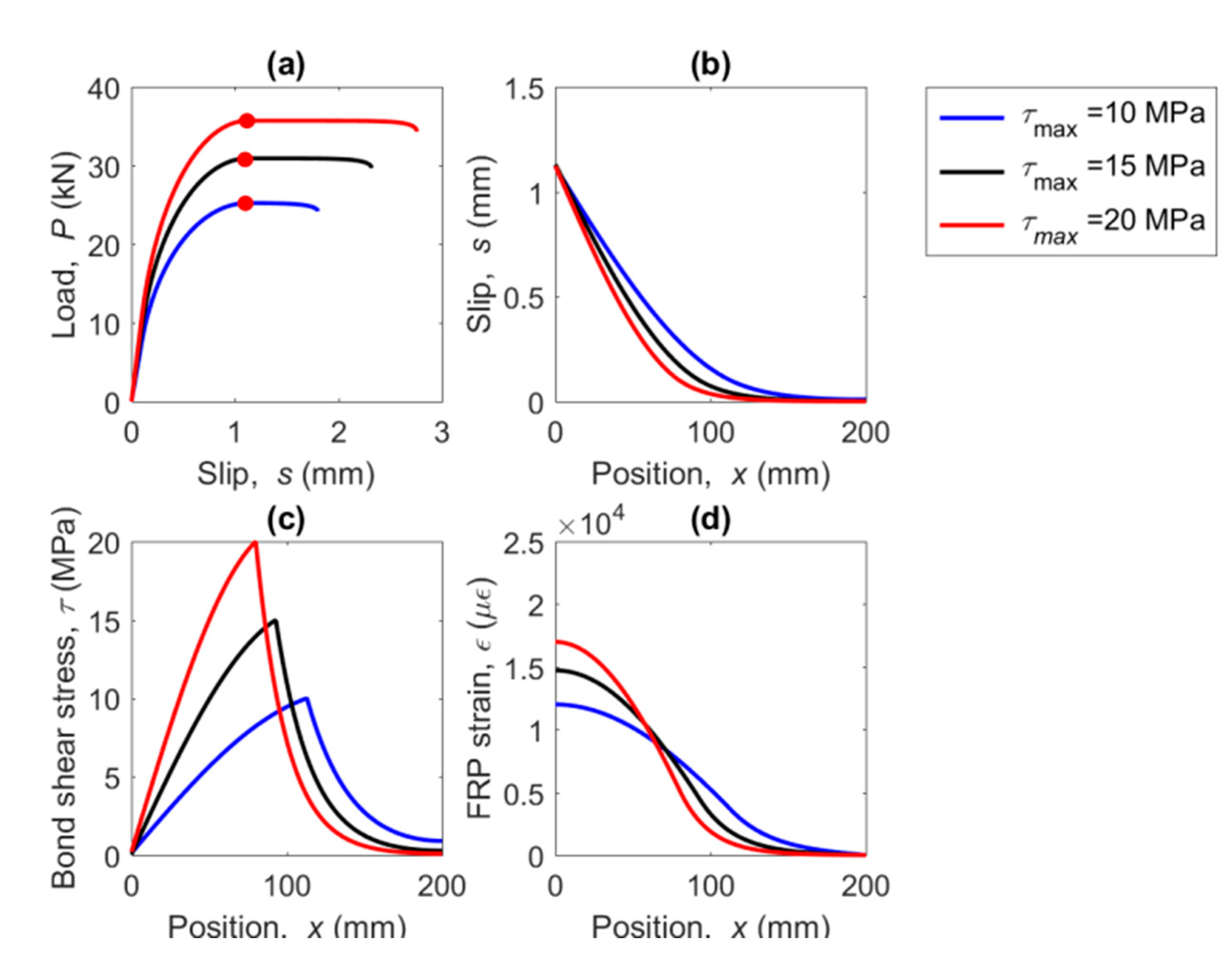
7.1. Effect of the Bond–Shear Strength (τmax)

Using the numerical model, the load–slip curve, and the slip, bond–shear stress and FRP strain profile along the bonded length are obtained. For the sake of brevity, only the response of the BL model is shown in Figure 14, however, the trends observed for the BL model can be extrapolated to the other bond–slip models. A range of τmax between 10 MPa and 20 MPa has been considered taking τmax,0 = 10 MPa as a reference for normalization of results and, being sf = 1.13 mm, s1 = 0.1 mm, s2 = 0.12 mm, and τf = 5.25 MPa.
In Figure 14, the curves are represented for the situation where the slip at the loaded end arrives at sf. It is clearly seen that Pmax increases with τmax (Figure 14a). This is because an increase of τmax implies an increase of Gf, thus, a higher load is needed to damage the bonded joint. In Figure 14b, where the slip profile is shown, it can be observed that as the τmax increases, the activated bonded length decreases. At x = 200 mm the slip in the free end when τmax is 10 MPa, is equal to 0.0091 mm, but when τmax is 20 MPa, the slip in the free end is negligible, meaning that the activated length decreases with the increase of τmax.
In Figure 14c the bond stress profile is represented. In that case, it can be seen that as τmax increases, the bond–shear profile becomes narrower because every segment along the bonded length is able to transfer a larger bond–shear force. Finally, as the bond–shear strength (τmax) increases, the strain in the loaded end increases as well (Figure 14d). It is worth noticing that as the bond–shear strength capacity increases, the activated bonded length decreases.
In Figure 15, the increase of the maximum load is depicted in function of the increase of the τmax, previously normalized with respect to τmax,0 = 10 MPa. In general terms, a practically linear increase of the maximum load with the bond–shear strength can be observed for all the models. This is due to the fact that increasing τmax without changing the value of sf causes a linear increase of the fracture energy (Gf), leading to a situation where a higher load is needed to damage the bonded joint.
Moreover, it can be seen that LD, BL, and TSANL models show very similar results, meaning that these models are analogously affected by the increase of the bond–shear strength. These models show an increase of Pmax of 41% when τmax is 20 MPa. Finally, BLF, BO, and BONP, show lesser effect on the maximum load than the other models, because of the friction branch, which remains constant for all the cases. Although these models increase their Gf, the increase of the area under the bond–slip curve is smaller than in the non-friction cases. The increase of Pmax in these models arrives to 30% when τmax is 20 MPa. Finally, the BLF model is slightly less affected than BO and BONP models, because of the non-linear ascending branch of Borchert models, which experiment a higher increase of Gf when τmax increases.
The influence of τmax on the effective length, Leff, is shown in Figure 16 for models without friction. In general, a decrease of its value is observed as τmax increases, as expected: if the bond–shear strength increases, every finite element of the bonded length can transfer a larger shear force, hence, less bonded length is needed to transfer the total load. It is worth noticing that the three models behave in a very similar way, indicating that assuming either the one stage model, the bilinear model or the model with a non-linear ascending stage, does not provide a difference on the effective bonded length for different bond strengths.

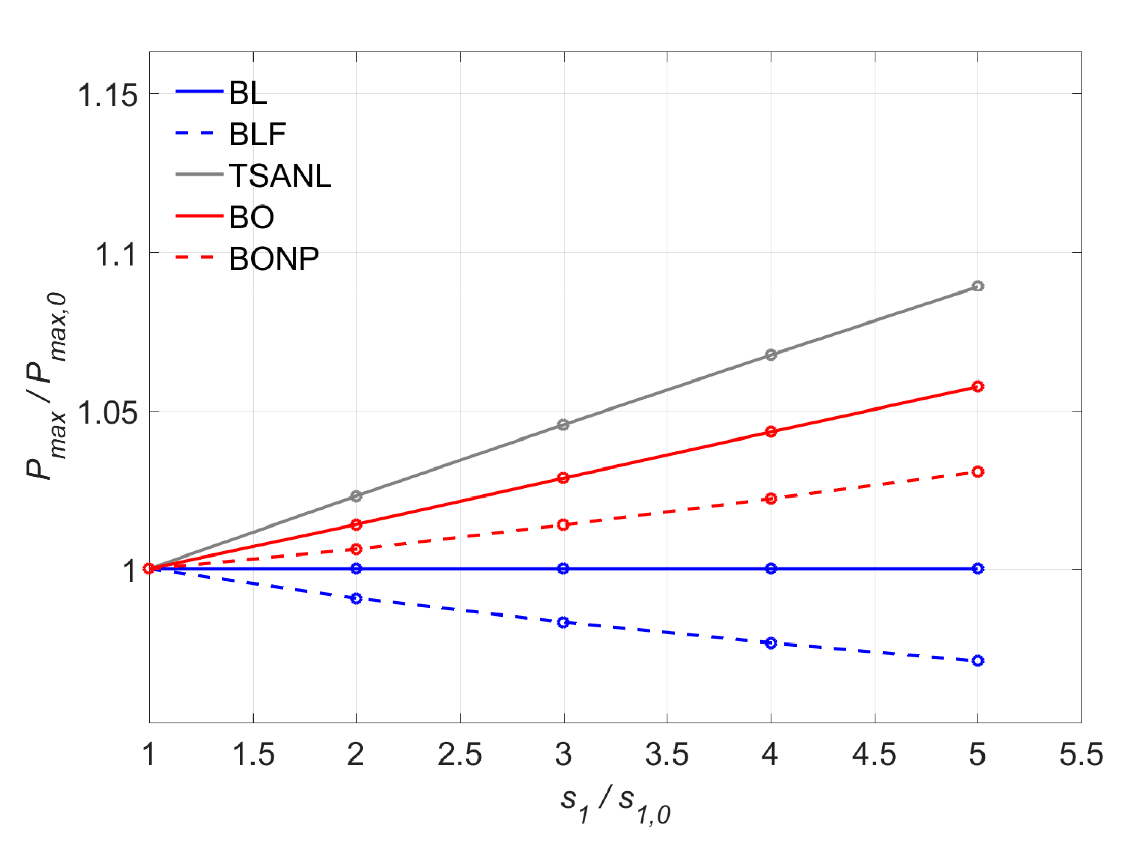
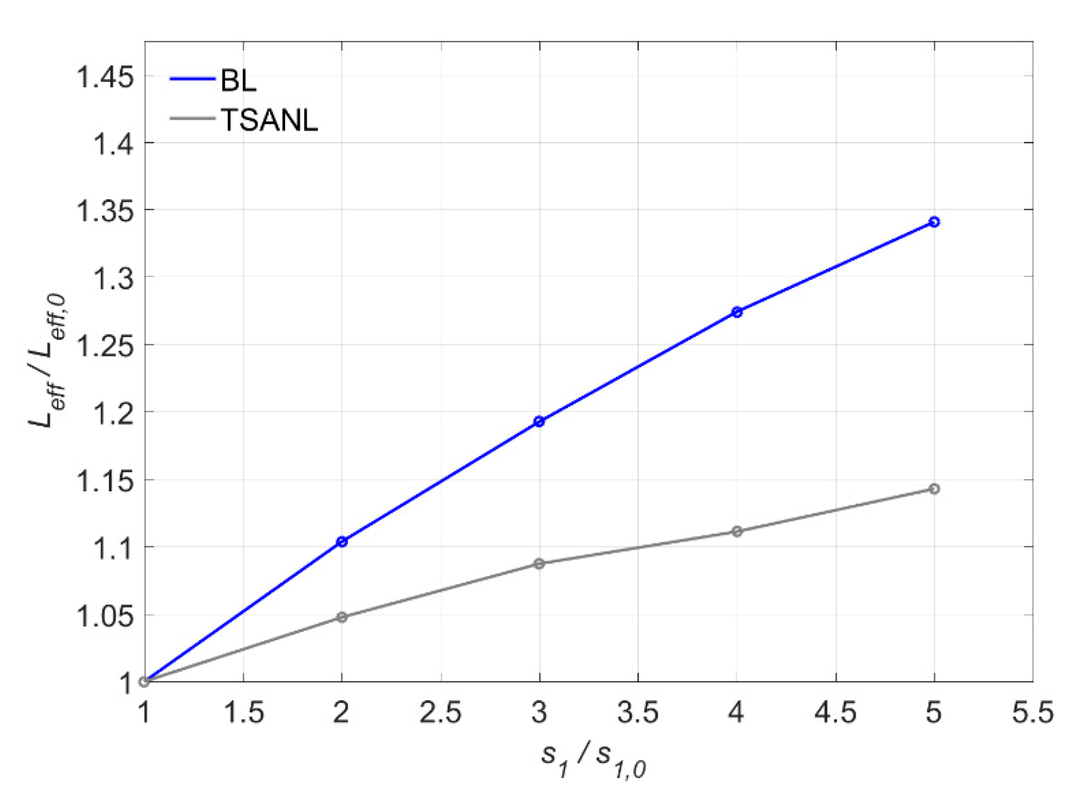
7.2. Effect of the Slip at the Bond–Shear Strength (s1)

A range for s1 between 0.1 mm and 0.5 mm has been considered, taking s1,0 = 0.1 mm for normalization of results, and keeping τmax = 15 MPa. The value of the Gf when s1,0 = 0.1 mm is equal to 8.5 N/mm. In order to meet the new value of s1, Gf varies between 8.5 N/mm and 10.9 N/mm, depending on the model considered. In BO model, the difference between s1 and s2 has been kept constant for all cases. The linear descending (LD) model is not included because the slip at the bond–shear strength is 0, and if this point is shifted horizontally, it would become a bilinear (BL) model.
The results are plotted in Figure 17 in terms of increment of the maximum load with respect to the increment of s1. As observed, in all models the load increment is considerably small (with a maximum variation of 8.9%). For the BL model, no effect on the maximum load is obtained for a substantial increment of s1, because τmax and sf are constant, and therefore, the fracture energy (Gf) remains the same.
In the case of the BLF model, the maximum load decreases as the s1 increases. Even though the fracture energy (Gf) remains constant for all the s1 values, as can be seen in Table 3, the area under the total bond shear–slip curve, considering the three stages (elastic, softening and friction) sligthly decreases with the increment of s1. It should be noticed, however, that the maximum load decrease only arrives up to 3% of the initial load.
It is also seen that bond–slip models that have a non-linear ascending branch (TSANL, BO, and BONP models) exhibit an some increase on the maximum load (Pmax), caused by the increase of area under the elastic stage curve from the shifting of s1. This effect can be observed in Table 3 through an increment of the fracture energy (Gf) with the increase of s1. It should be noticed that the variation of the fracture energy for TSANL and BONP models is the same, therefore, in Table 3, only BONP model is showed. In BO and BONP cases, the increase of the fracture energy is mitigated by the decreasing of friction area between s3 and sf (Table 1): since the value of sf is kept constant and s1 increases, the value of s3 shifts horizontally, causing a reduction of area between s3 and sf.
The TSANL model is more affected by the modification of s1 than the other models, since it does not have a friction branch and the total area under the bond–slip law will not decrease with the shifting of s1, and the increase of the fracture energy will not be mitigated. The increase of Gf in the TSANL model is the same as in the BONP model, since the definition of Gf has been considered as in Figure 5.
Figure 18 shows the variation of the effective bonded length with s1 for TSANL and BL models. The effective bonded length (Leff) increases as s1 increases. Since higher slips are obtained in the elastic stage, a longer bonded length will be activated and Leff will increase.
Moreover, the BL model is more sensitive to the variation of s1 than the TSANL model, because the change in the non-linear ascending branch of the TSANL model slightly increases the area under the elastic branch, improving the resistance of the joint under in this stage. This way, the increase of slip caused by the s1 shifting is mitigated by this increase of resistance.

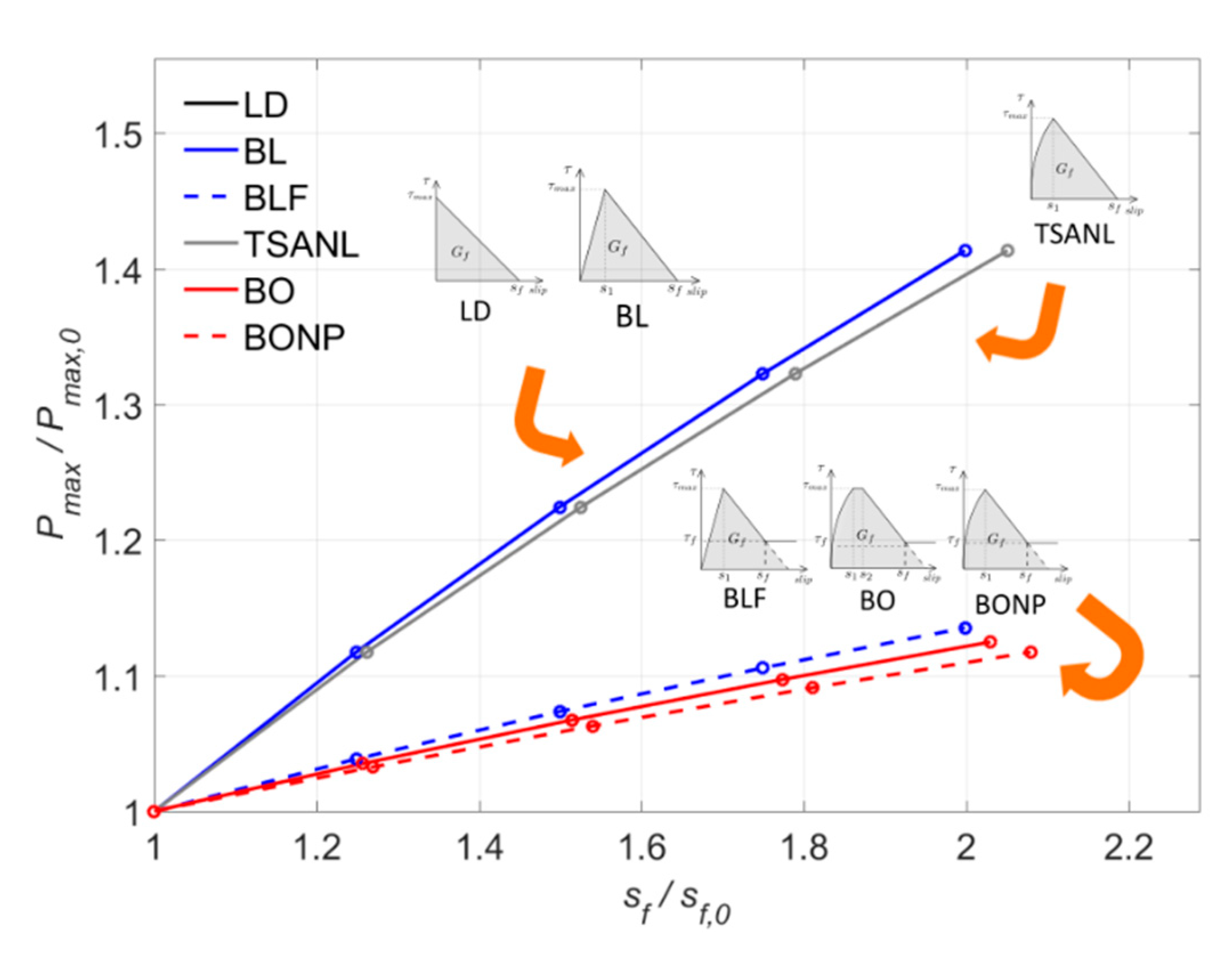
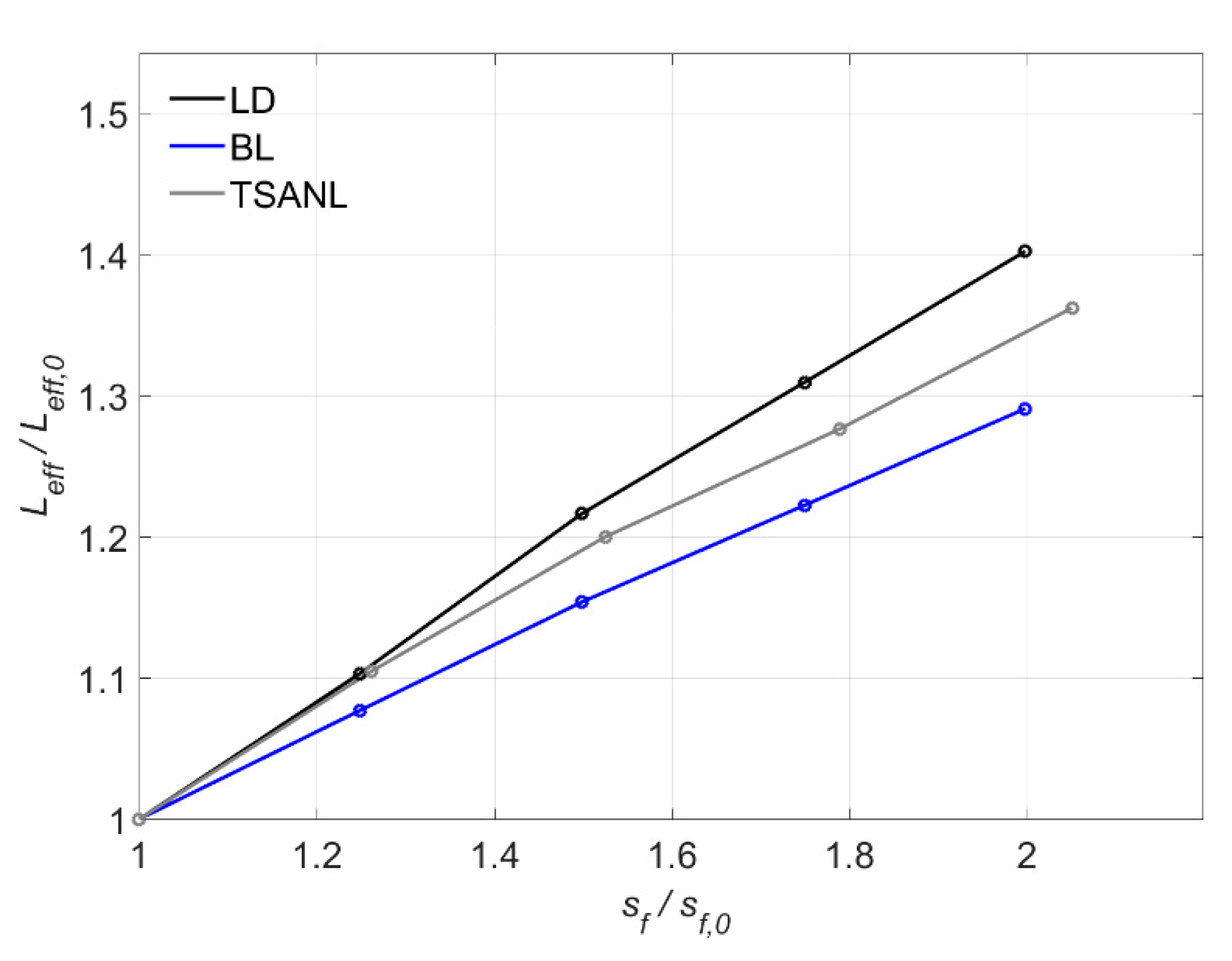
7.3. Effect of the Maximum Slip (sf)

Fixing the values of the bond–shear strength (τmax) and the slip at the b ond shear strength (s1) to 15 MPa and 0.1 mm, respectively, and setting the fracture energy (Gf) to the values obtained in Section 7.1 (ranging between 8.5 N/mm and 11.33 N/mm) for each model, the values of the initial maximum slip (sf,0) are between 0.70 mm and 0.75 mm. Because the bond–slip models have different shapes, and therefore, different values of Gf, the maximum slip, which satisfies the conditions of τmax and s1, will be different for each bond–slip law, as seen in Figure 19.
Overall, in Figure 19 it can be seen that all the models show an increasing tendency of Pmax with sf, because as sf increases, Gf increases as well. The LD model presents exactly the same curve as the BL, since in both cases Gf is the same. Moreover, as indicated in previous subsections, models without friction branch—such as LD, BL, and TSANL—are more sensitive to the increase of sf because the shifting of the slip affects directly to Gf, Pmax increases up to 41% when sf is the highest value. It is worth noticing that the TSANL is slightly less sensitive because the area under the elastic branch is higher than in LD and BL models, causing that the increment of sf affects proportionally less to Gf and Pmax, around 13% when sf is the maximum value. As for the models with friction branch—BLF, BO, and BONP—increase the Pmax caused by the shifting of sf is diminished by the effect of the friction branch in the total area as indicated in previous subsections.
Figure 20 shows that Leff increases with the increase of sf for all models. A higher sf allows the bonded joint to have higher slips while transferring load, and consequently, more bonded length is activated. LD model exhibits the highest influence of sf and BL model is the less affected model.

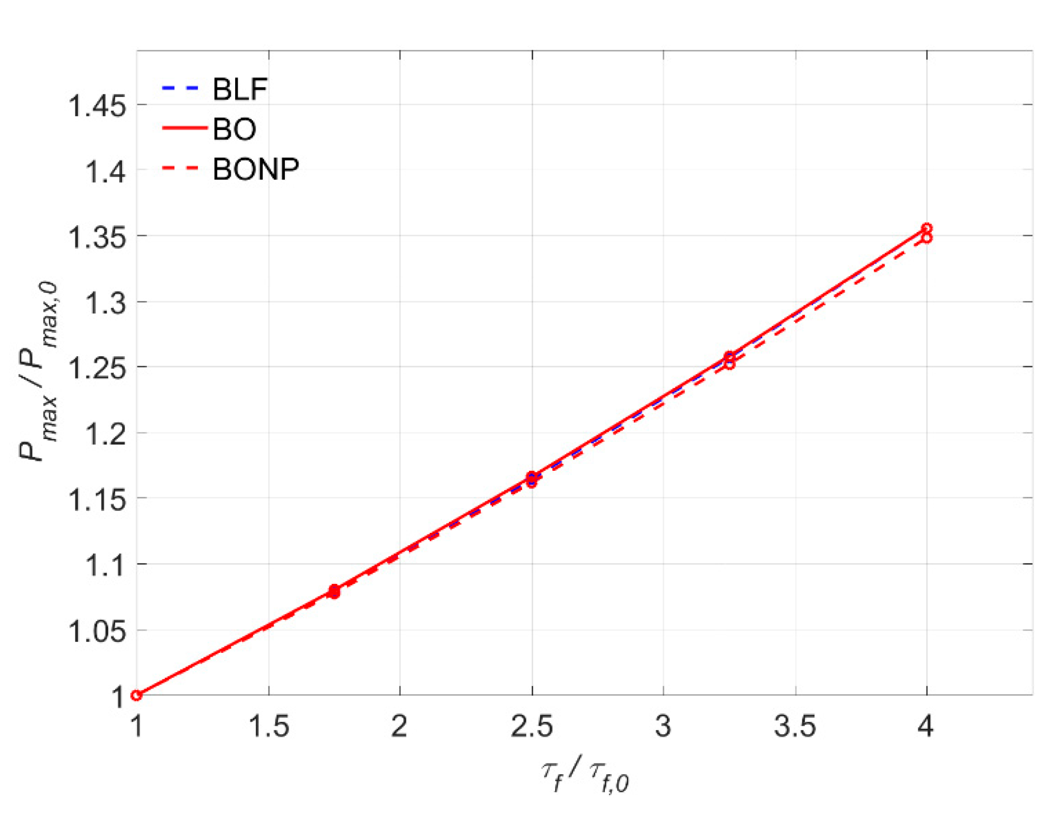
7.4. Effect of the Friction Branch (τf)

Only BLF, BO, and BONP (with friction branch) models are included in this section. The bond–slip law parameters are set to τmax = 15 MPa, s1 = 0.1 mm, and Gf = 8.5 N/mm. The bond–shear stress of the friction branch ranges between 10% and 40% of τmax, therefore τf will vary between 1.5 MPa (τf,0) and 6 MPa.
Figure 21 shows the variation of Pmax with the increase of τf. It can be seen that all models present the same almost linear rising tendency, as expected. For example, for an increase of 2.5 times τf,0 (i.e., τf = 3 MPa), the increase of Pmax is around 17%, while for 4 times τf,0 (τf = 6 MPa), Pmax increases around 35%.

8. Conclusions

A study on the effect of the local bond–slip law characterizing the material bond behavior and its parameters on the global structural bond response of NSM FRP strengthened RC elements has been presented. A numerical method has been developed in order to being able to solve the governing equations of the bonded joint for any type of bond–slip law.
From the comparison between the results of the different bond–slip laws, the following conclusions are obtained:
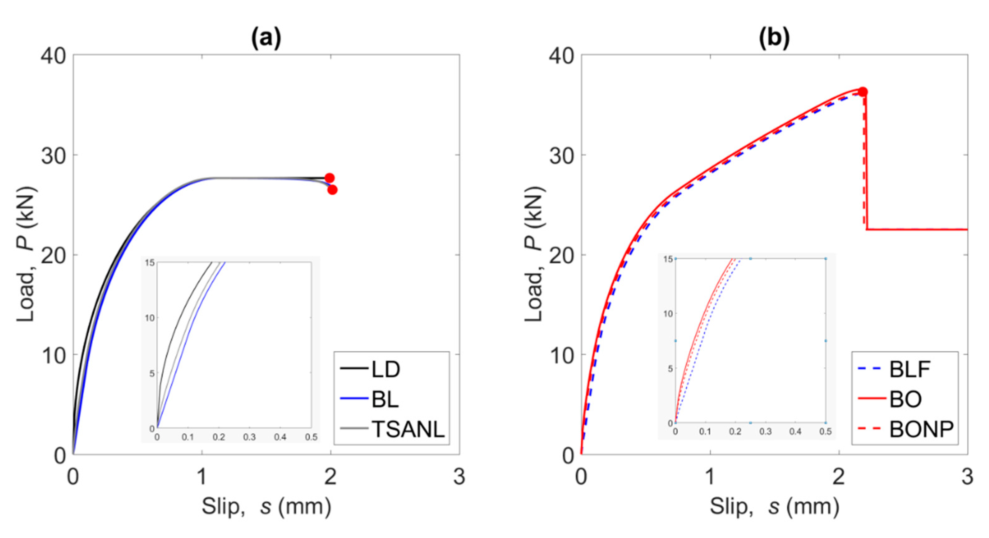
  • In models not including a friction branch after softening, a maximum value of load is attained, which stabilizes for a certain value of the bonded length. In contrast, in models with friction component, the load continuously increases up to a certain slip beyond which only the friction component remains. Furthermore, models with non-linear ascending branch show a stiffener initial load–slip response.
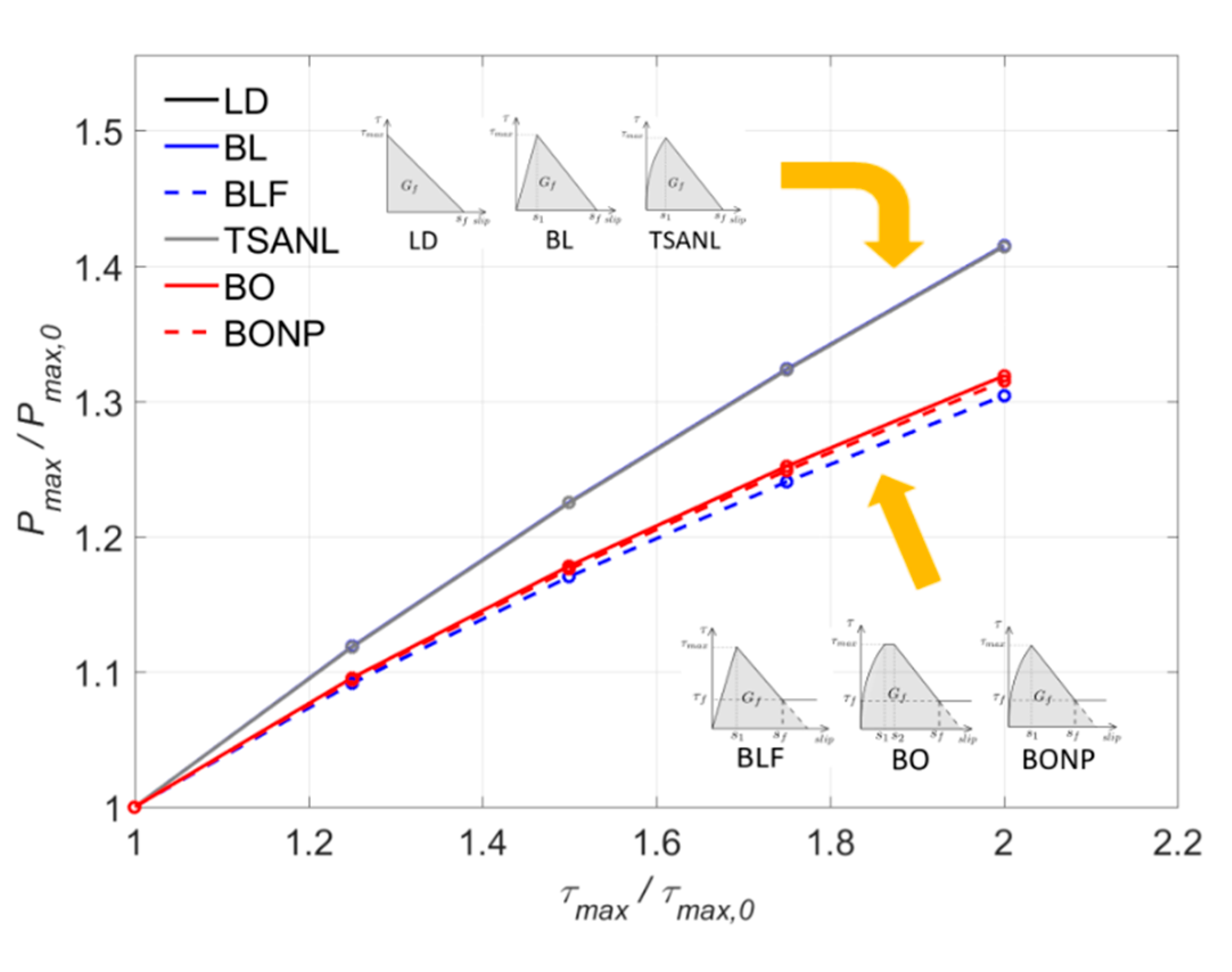
  • The non-linear ascending branch effect on the maximum load is practically negligible. Small differences of Pmax are observed between BL and TSANL models, and BLF and BONP models, respectively.
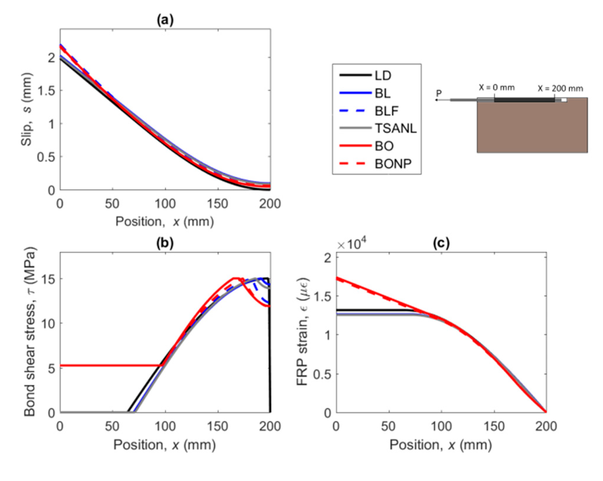
  • The shape of the bond–slip law has a small effect on the slip profile along the FRP. However, the bond stress and slip distribution at maximum state along the bonded length is strongly affected by the friction branch.
  • From the comparison between numerical and experimental results, it can be concluded that:
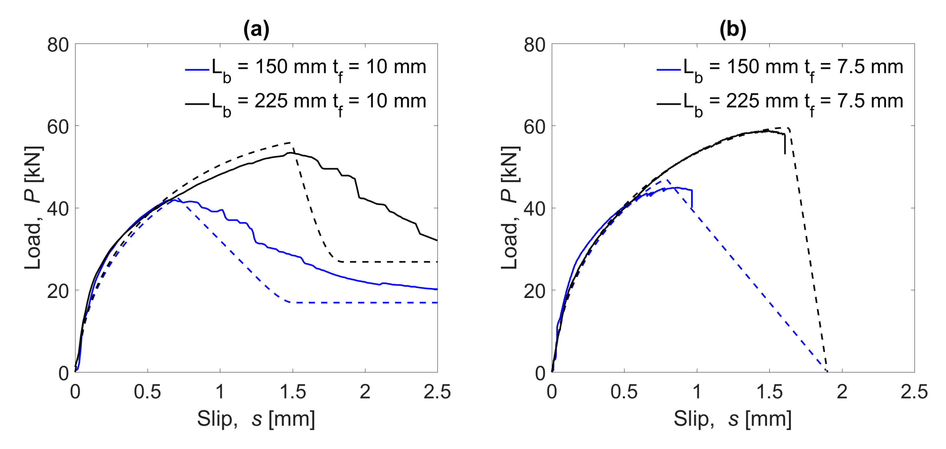
  • A close agreement between the finite differences model and the experimental results is obtained. The comparison between the load–slip curves obtained experimentally and numerically showed that the ascending part is correctly predicted until failure.
  • A somewhat larger maximum load of around 7–10% was obtained for specimens with 7.5 mm groove thickness compared to those with 10 mm. As the groove thickness decreased, the maximum load of the bonded joint increased.
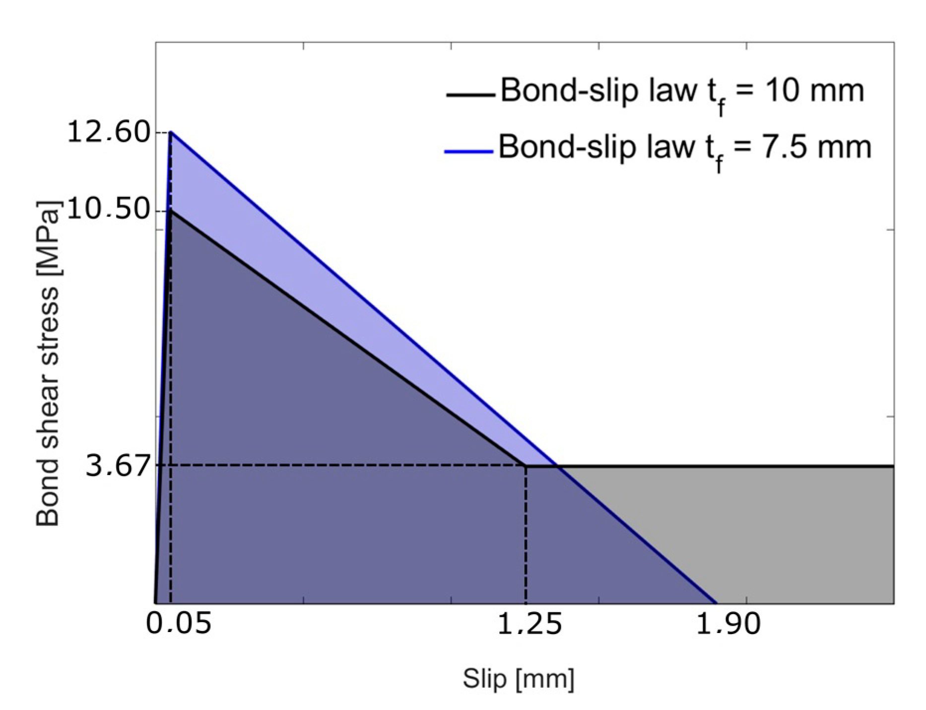
  • Specimens with 10 mm groove thickness showed a behavior indicating the existence of a friction branch in their local bond law and the failure was in the FRP-adhesive interface. Conversely, the behavior of 7.5 mm groove thickness specimens was properly described using a bilinear function, while the failure was in the resin–concrete interface.
  • From the parametric study carried out, the following conclusions can be drawn:
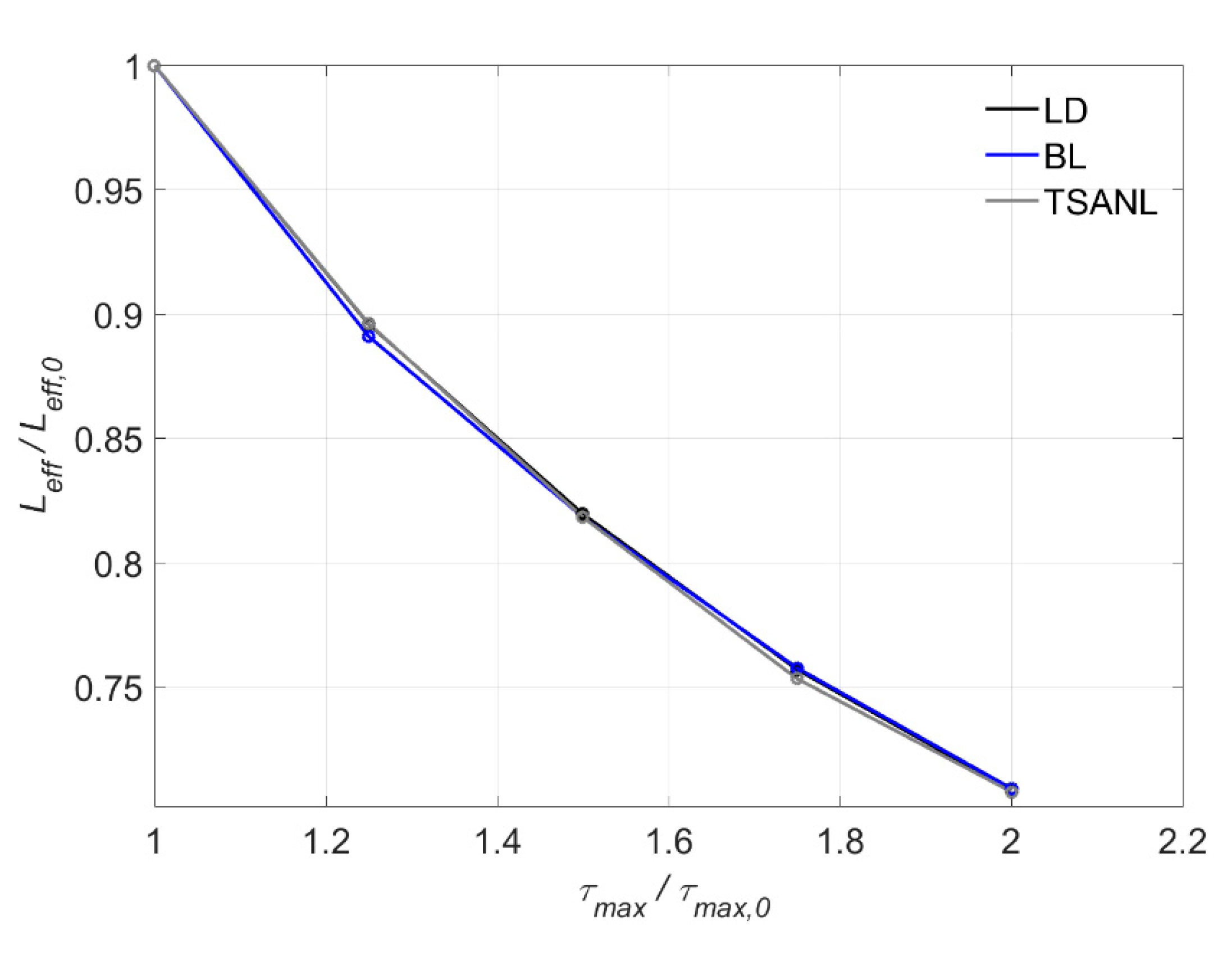
  • As the bond–shear strength increases, the maximum load grows, and conversely, the effective bonded length decreases.
  • The slip at the bond shear strength, s1, has a small effect on the maximum load and an increasing effect on the effective bonded length.
  • The maximum load and the effective bonded length increase with the maximum slip. Moreover, bond–slip laws without friction branch are much more sensitive to the shifting of the maximum slip.
  • The presence of a friction stage in the local bond behavior causes an increase on the maximum load. As the bond–shear strength on the friction branch increases, the maximum load increases as well.

Author Contributions

Conceptualization, validation and formal analysis, J.G., C.B. and L.T.; methodology and investigation, J.G., C.B. and L.T.; writing—original draft preparation, J.G.; writing—review and editing, J.G., C.B. and L.T.; supervision, C.B. and L.T.; funding acquisition, C.B. and L.T. All authors have read and agreed to the published version of the manuscript.

Funding

This research was funded by the Spanish Government (MINECO), Project Ref. BIA2017-84975-C2-2-P.

Acknowledgments

The first author acknowledges the University of Girona for the IFUdG grant IFUDG2018/28. The authors also thank the support of SIKA Services AG for the supply of materials used in this study.

Conflicts of Interest

The authors declare no conflict of interest.

References

  1. fib Bulletin 90. Externally Applied FRP Reinforcement for Concrete Structures. International Federation for Structural Concrete; fib Bulletin: Lausanne, Switzerland, 2019. [Google Scholar]
  2. De Lorenzis, L.; Teng, J.G. Near-surface mounted FRP reinforcement: An emerging technique for strengthening structures. Compos. Part B Eng. 2007, 38, 119–143. [Google Scholar] [CrossRef]
  3. Yuan, H.; Teng, J.G.; Seracino, R.; Wu, Z.S.; Yao, J. Full-range behavior of FRP-to-concrete bonded joints. Eng. Struct. 2004, 26, 553–565. [Google Scholar] [CrossRef]
  4. Yuan, H.; Lu, X.; Hui, D.; Feo, L. Studies on FRP-concrete interface with hardening and softening bond–slip law. Compos. Struct. 2012, 94, 3781–3792. [Google Scholar] [CrossRef]
  5. Ali, M.S.M.; Oehlers, D.J.; Griffith, M.C.; Seracino, R. Interfacial stress transfer of near surface-mounted FRP-to-concrete joints. Eng. Struct. 2008, 30, 1861–1868. [Google Scholar]
  6. Chen, J.F.; Teng, J.G. Anchorage strength models for FRP and steel plates. J. Struct. Eng. 2001, 127, 784–791. [Google Scholar] [CrossRef]
  7. D’Antino, T.; Pellegrino, C. Bond between FRP composites and concrete: Assessment of design procedures and analytical models. Compos. Part B Eng. 2014, 60, 440–456. [Google Scholar] [CrossRef]
  8. Ferracuti, B.; Savoia, M.; Mazzotti, C. A numerical model for FRP-concrete delamination. Compos. Part B Eng. 2006, 37, 356–364. [Google Scholar] [CrossRef]
  9. Lu, X.Z.; Teng, J.G.; Ye, L.P.; Jiang, J.J. Bond–slip models for FRP sheets/plates bonded to concrete. Eng. Struct. 2005, 27, 920–937. [Google Scholar] [CrossRef]
  10. Biscaia, H.C.; Chastre, C.; Silva, M.A.G. Linear and nonlinear analysis of bond–slip models for interfaces between FRP composites and concrete. Compos. Part B Eng. 2013, 45, 1554–1568. [Google Scholar] [CrossRef]
  11. Soares, S.; Sena-Cruz, J.; Cruz, J.R.; Fernandes, P. Influence of surface preparation method on the bond behavior of externally bonded CFRP reinforcements in concrete. Materials (Basel) 2019, 12, 414. [Google Scholar] [CrossRef] [Green Version]
  12. Yin, Y.; Fan, Y. Influence of roughness on shear bonding performance of CFRP-concrete interface. Materials (Basel). 2018, 11, 1875. [Google Scholar] [CrossRef] [Green Version]
  13. Sena-Cruz, J.; Barros, J.A.O. Bond between Near-surface mounted carbon-fiber-reinforced polymer laminate strips and concrete. J. Compos. Constr. 2004, 8, 519–527. [Google Scholar] [CrossRef] [Green Version]
  14. Borchert, K.; Zilch, K. Bond behavior of NSM FRP strips in service. Struct. Concr. 2008, 9, 127–142. [Google Scholar] [CrossRef]
  15. Zhang, S.S.; Teng, J.G.; Yu, T. Bond–slip model for interfaces between near-surface mounted CFRP strips and concrete. In Proceedings of the 11th International Symposium on Fiber Reinforced Polymers for Reinforced Concrete Structures (FRPRCS-11), Guimarães, Portugal, 26–28 June 2013; pp. 1–7. [Google Scholar]
  16. Seracino, R.; Raizal Saifulnaz, M.R.; Oehlers, D.J. Generic debonding resistance of EB and NSM plate-to-concrete joints. J. Compos. Constr. 2007, 11, 62–70. [Google Scholar] [CrossRef]
  17. Zilch, K.; Borchert, K. A general bond stress slip relationship for NSM FRP strips. In Proceedings of the 8th International Symposium on FRP Reinforcement for Concrete Structures, Patras, Greece, 16–18 July 2007. [Google Scholar]
  18. Finckh, W.; Zilch, K. Strengthening and rehabilitation of reinforced concrete slabs with carbon-fiber reinforced polymers using a refined bond model. Comput. Civ. Infrastruct. Eng. 2012, 27, 333–346. [Google Scholar] [CrossRef]
  19. Zilch, K.; Niedermeier, R.; Finckh, W. Strengthening of Concrete Structures with Adhesively Bonded Reinforcement; Ernst & Shon: Berlin, Germany, 2014. [Google Scholar]
  20. D’Antino, T.; Colombi, P.; Carloni, C.; Sneed, L.H. Estimation of a matrix-fiber interface cohesive material law in FRCM-concrete joints. Compos. Struct. 2018, 193, 103–112. [Google Scholar] [CrossRef]
  21. Zou, X.; Sneed, L.H.; D’Antino, T. Full-range behavior of fiber reinforced cementitious matrix (FRCM)-concrete joints using a trilinear bond–slip relationship. Compos. Struct. 2020, 239, 112024. [Google Scholar] [CrossRef]
  22. Torres, L.; Sharaky, I.A.; Barris, C.; Baena, M. Experimental study of the influence of adhesive properties and bond length on the bond behavior of NSM FRP bars in concrete. J. Civ. Eng. Manag. 2016, 22, 808–817. [Google Scholar] [CrossRef] [Green Version]
  23. Sharaky, I.A.; Torres, L.; Baena, M.; Miàs, C. An experimental study of different factors affecting the bond of NSM FRP bars in concrete. Compos. Struct. 2013, 99, 350–365. [Google Scholar] [CrossRef]
  24. Ko, H.; Matthys, S.; Palmieri, A.; Sato, Y. Development of a simplified bond stress-slip model for bonded FRP-concrete interfaces. Constr. Build. Mater. 2014, 68, 142–157. [Google Scholar] [CrossRef]
  25. Bilotta, A.; Ceroni, F.; Barros, J.A.O.; Costa, I.; Palmieri, A.; Szabó, Z.K.; Nigro, E.; Matthys, S.; Balazs, G.L.; Pecce, M. Bond of NSM FRP-strengthened concrete: Round robin test initiative. J. Compos. Constr. 2015, 20, 04015026. [Google Scholar] [CrossRef] [Green Version]
  26. Ceroni, F.; Pecce, M.; Bilotta, A.; Nigro, E. Bond behavior of FRP NSM systems in concrete elements. Compos. Part B Eng. 2012, 43, 99–109. [Google Scholar] [CrossRef]
  27. Haskett, M.; Oehlers, D.J.; Ali, M.S.M. Local and global bond characteristics of steel reinforcing bars. Eng. Struct. 2008, 30, 376–383. [Google Scholar] [CrossRef]
  28. UNE 12390-3. Testing Hardened Concrete. Part 3: Compressive Strength of Test Specimens; AENOR: Madrid, Spain, 2003. [Google Scholar]
  29. ASTM C469/C469M-10. Standard Test Method for Static Modulus of Elasticity and Poisson’s Ratio of Concrete in Compression; ASTM International: West Conshohocken, PA, USA, 2010. [Google Scholar]
  30. ISO 527-5:2009. Determination of Tensile Properties—Part 5: Test Conditions for Unidirectional Fiber-Reinforced Plastic Composites; ISO: Geneva, Switzerland, 2009. [Google Scholar]
  31. ISO 527-2:2012. Determination of Tensile Properties-Part 2: Test Conditions for Moulding and Extrusion Plastics. International Organisation for Standardization (ISO); ISO: Geneva, Switzerland, 2012. [Google Scholar]
  32. ACI 440.2R-17. Guide for the Design and Construction of Externally Bonded FRP Systems for Strengthening Existing Structures; American Concrete Institute: Farmington Hills, MI, USA, 2017. [Google Scholar]
  33. Seracino, R.; Jones, N.M.; Ali, M.S.; Page, M.W.; Oehlers, D.J. Bond strength of near-surface mounted FRP strip-to-concrete joints. J. Compos. Constr. 2007, 11, 401–409. [Google Scholar] [CrossRef]
  34. Zhang, S.S.; Teng, J.G.; Yu, T. Bond strength model for CFRP strips near-surface mounted to concrete. J. Compos. Constr. 2014, 18, A4014003. [Google Scholar] [CrossRef]
  35. Savoia, M.; Mazzotti, C.; Ferracuti, B. A new single-shear set-up for stable debonding of FRP-concrete joints. Constr. Build. Mater. 2009, 23, 1529–1537. [Google Scholar]
  36. Emara, M.; Torres, L.; Baena, M.; Barris, C.; Cahís, X. Bond response of NSM CFRP strips in concrete under sustained loading and different temperature and humidity conditions. Compos. Struct. 2018, 192, 1–7. [Google Scholar] [CrossRef]
Figure 1. Stress equilibrium (a) in the FRP-concrete joint, and (b) in the FRP-adhesive interface.
Materials 13 01770 g001
Figure 2. Scheme of the discretization along the FRP.
Materials 13 01770 g002
Figure 3. Flowchart of the numerical procedure.
Materials 13 01770 g003
Figure 4. Comparison between the analytical and the numerical models.
Materials 13 01770 g004
Figure 5. Fracture energy obtained from the bond–slip law.
Materials 13 01770 g005
Figure 6. Comparison of the bond–slip models.
Materials 13 01770 g006
Figure 7. Comparison of the load–slip curves, (a) shows LD, BL and TSANL models, and (b) shows BLF, BO, and BONP models.
Materials 13 01770 g007
Figure 8. (a) FRP slip, (b) bond–shear stress, and (c) FRP strains along the bonded length for the different bond–slip models.
Materials 13 01770 g008
Figure 9. (a) scheme of the set-up for the pull-out single shear test, and (b) picture of the tests.
Materials 13 01770 g009
Figure 10. Experimental results from the single shear tests.
Materials 13 01770 g010
Figure 11. Bond–slip law parameters obtained from the load–slip curve for 7.5 mm grooved specimens.
Materials 13 01770 g011
Figure 12. Experimental bond–slip laws for the NSM with 7.5 mm and 10 mm thickness grooves.
Materials 13 01770 g012
Figure 13. Comparison between the experimental (continuous lines) and the theoretical (dashed lines) values for the NSM with (a) 10 mm and (b) 7.5 mm groove thickness.
Materials 13 01770 g013
Figure 14. (a) Load–slip curve, (b) slip along the FRP, (c) bond–shear stress along the FRP, and (d) strains along the FRP for three values of bond–shear strength and a bilinear bond–slip law.
Materials 13 01770 g014
Figure 15. Variation of Pmax versus τmax.
Materials 13 01770 g015
Figure 16. Variation of Leff versus τmax.
Materials 13 01770 g016
Figure 17. Variation of Pmax versus s1.
Materials 13 01770 g017
Figure 18. Variation of Leff versus s1.
Materials 13 01770 g018
Figure 19. Variation of Pmax versus sf.
Materials 13 01770 g019
Figure 20. Variation of Leff versus sf.
Materials 13 01770 g020
Figure 21. Variation of Pmax versus τf.
Materials 13 01770 g021
Table 1. Equations of the bond–slip models used in the parametric study.
Bond–Slip ModelEquation
Linear Descending (LD)
Materials 13 01770 i001
τ ( s ) = {   τ m a x * ( s f s ) s f , s > 0   a n d   s   s f   0 , s     s f
Bilinear (BL)
Materials 13 01770 i002
τ ( s ) = { τ m a x * s s 1 , s < s 1   τ m a x * ( s f s ) ( s f s 1 ) , s > s 1   a n d   s   s f     0 , s     s f
Bilinear-friction (BLF)
Materials 13 01770 i003
τ ( s ) = { τ m a x * s s 1 , s < s 1   τ m a x * ( s f s ) ( s f s 1 ) , s > s 1   a n d   s   s 3     τ f , s     s 3
Two-stage ascending non-linear (TSANL)
Materials 13 01770 i004
τ ( s ) = { τ m a x * ( s s 1 ) , s < s 1   τ m a x * ( s f s ) ( s f s 1 ) , s > s 1   a n d   s   s f     0 , s     s f
Borchert (BO)
Materials 13 01770 i005
τ ( s ) = { τ m a x * ( s s 1 ) , s < s 1 τ m a x , s s 1   a n d   s s 2   τ m a x ( τ m a x τ f ) ( s f s 1 ) * ( s s 1 ) , s > s 2   a n d   s   s 3     τ f , s     s 3
Borchert no plateau (s1 = s2) (BONP)
Materials 13 01770 i006
τ ( s ) = { τ m a x * ( s s 1 ) , s < s 1   τ m a x ( τ m a x τ f ) ( s f s 1 ) * ( s s 1 ) , s > s 1   a n d   s   s 3     τ f , s     s 3
Note: τ = bond–shear stress; s = slip; τmax = bond–shear strength; s1 = slip when the bond–shear strength is achieved; s2 = final slip of the plateau; s3 = initial slip of the friction plateau; sf = maximum slip of the bonded joint; τf = friction bond–shear stress; α = experimental parameter that control the shape of the bond–slip law.
Table 2. Characteristics of the specimens
Specimen IDBonded Length (mm)Groove Thickness (mm)Maximum Load (kN)Failure Mode
NSM – 150 – 101501043.85F-A
NSM – 225 – 102251054.74F-A
NSM – 150 – 7.51507.547.14C-A
NSM – 225 – 7.52257.557.71C-A
Note: F-A = FRP-adhesive interface, C-A = concrete-adhesive interface.
Table 3. Variation of fracture energy for the BONP, BO and BLF models.
BONPBOBLF
s1[mm] s 1 s 1 , 0 ( G f G f , 0 G f , 0 ) * 100 ( G f G f , 0 G f , 0 ) * 100 ( G f G f , 0 G f , 0 ) * 100
0.1010 %0 %0 %
0.2024.64 %6.85 %0 %
0.3039.29 %13.71 %0 %
0.40413.94 %20.56 %0 %
0.50518.59 %27.42 %0 %

