Prediction of Static Modulus and Compressive Strength of Concrete from Dynamic Modulus Associated with Wave Velocity and Resonance Frequency Using Machine Learning Techniques


Abstract
1. Introduction
2. Materials and Methods
2.1. Materials and Preparation of Specimens
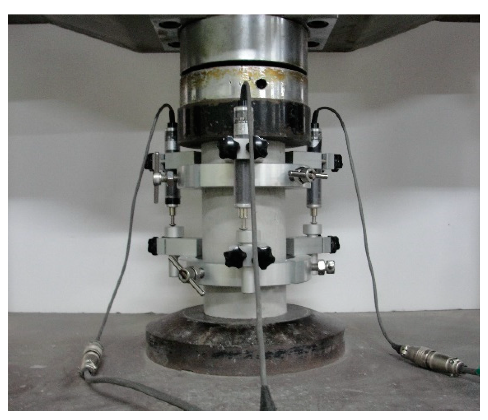
2.2. Static Tests for Elastic Modulus and Compressive Strength
2.3. P- and S-Wave Measurements for Calculating Dynamic Elastic Modulus
2.4. Resonance Frequency Tests for Calculating Dynamic Elastic Modulus
3. ML Techniques
3.1. SVM
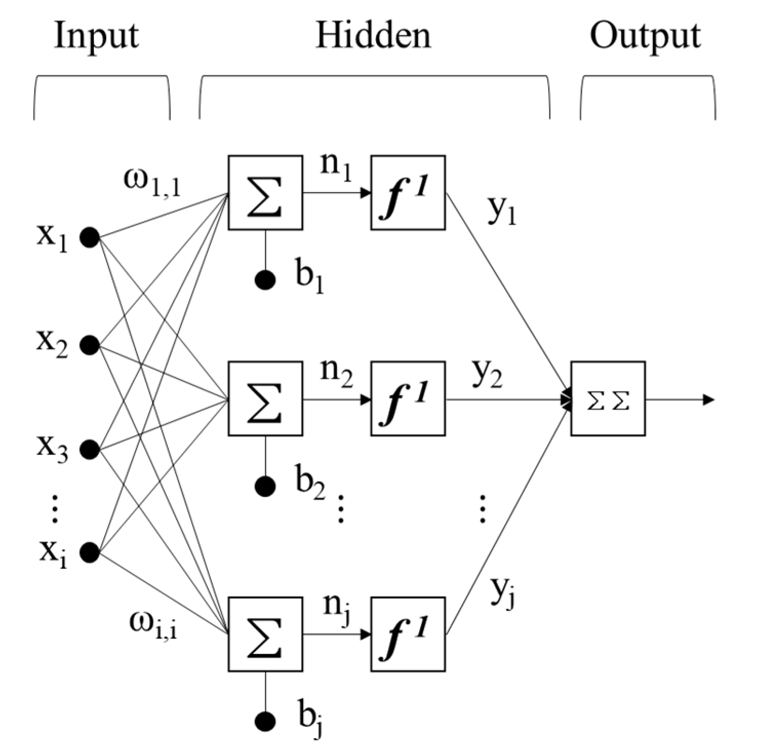
3.2. ANN
3.3. Ensemble
3.4. LR
4. Results and Discussion
4.1. Experimental Variability of Static and Dynamic Tests
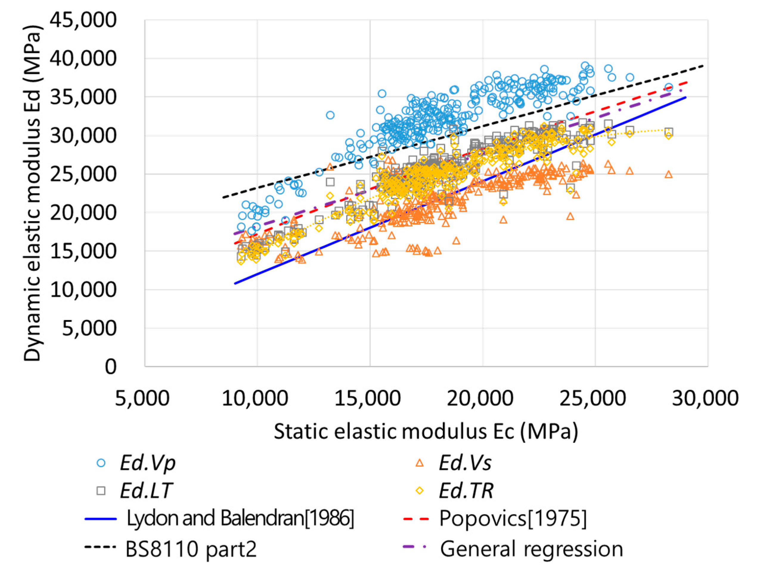
4.2. Relationship between Static and Dynamic Elastic Moduli
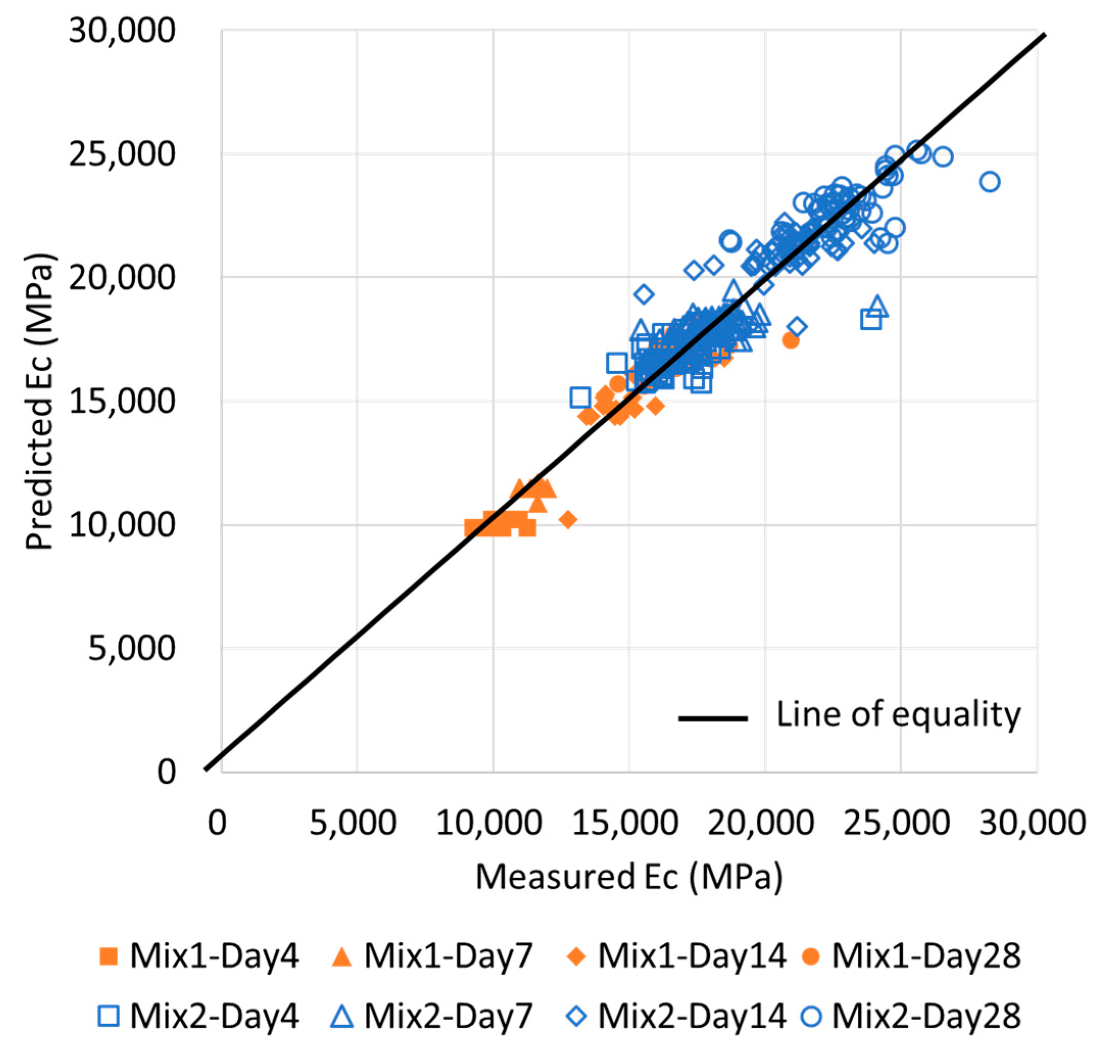
4.3. Comparison between Static and Prediction Elastic Moduli
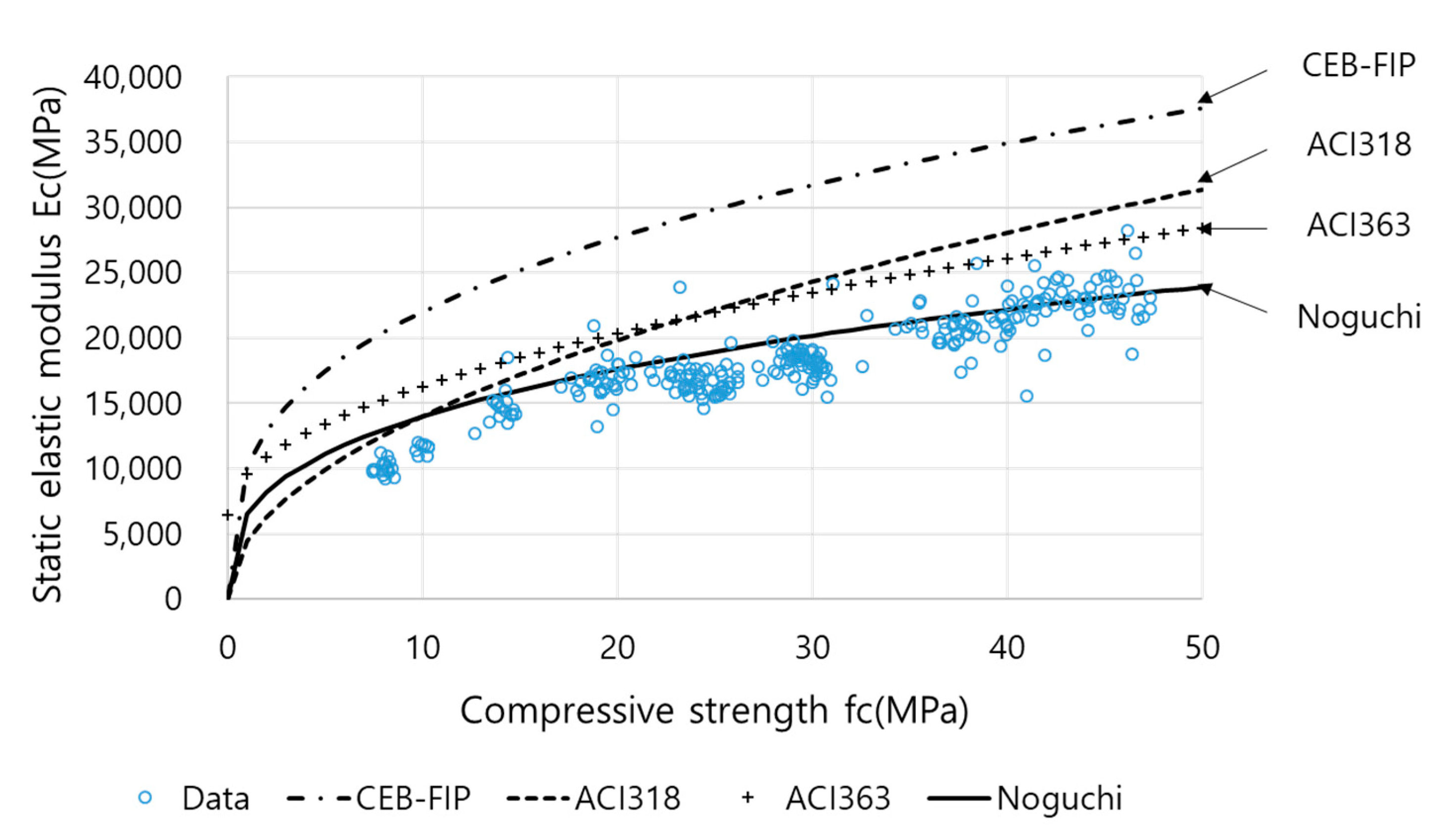
4.4. Relationship between Static Elastic Modulus and Compressive Strength
4.5. Relationship between Dynamic Elastic Modulus and Compressive Strength
4.6. Comparison between Predicted and Measured Values of Compressive Strength
5. Conclusions
- Among the four Eds, A is the largest, C and D are located in the middle, and B has the smallest value. The correlation with Ec and fc was identified as C > D > A > B.
- The Lydon and Balendran equation yields similar values to the B, and the Popovics equation provides results that are similar to the C and D. In addition, BS 8110 Part 2 yields similar values to the A.
- For the Ec and fc prediction results, the application of ML improved the accuracy by 2.5–5% and 7–9%, respectively, as compared with general regression.
- When Ec was predicted using the four Ed values, the order of accuracy of a single variable was C > D > A > B. The combination sets (B, C), (A, B, C), and (A, B, C, D) yielded the highest accuracy. Moreover, only the combination of B and C attained an accuracy level of up to 4.18%. Although B contained large-variance data for the early-age concrete, it complemented the most widely used and reliable C method.
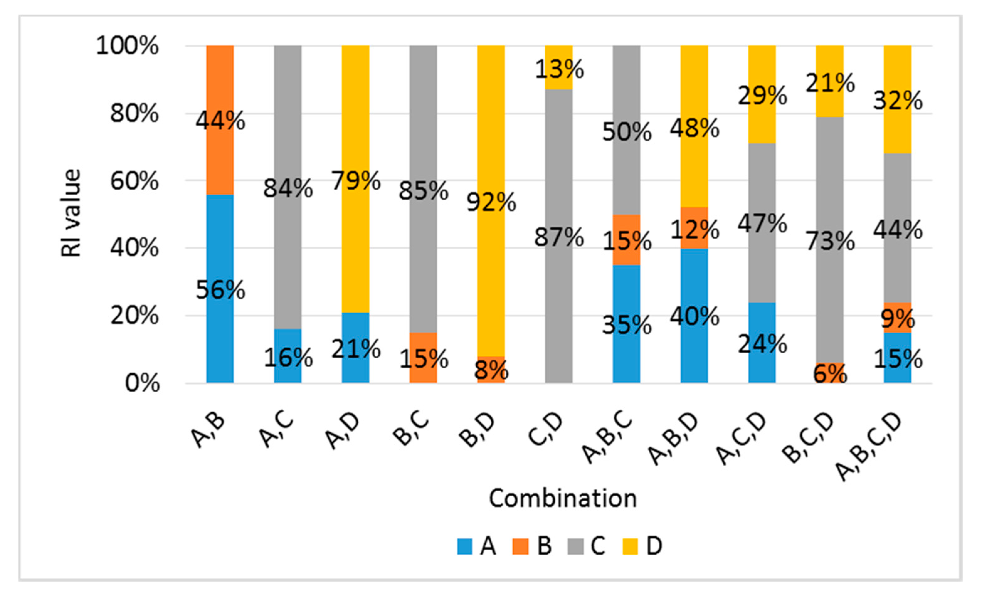
- When fc was predicted using the four Ed values, the order of accuracy of a single variable was C > D > A > B, which is similar to the order for the Ec values. The combinations of (B, C) and (B, D) were optimal, yielding accuracies of up to 5.90%. Although the variance in the B data was large for the prediction of fc, B was considered to be useful in supplementing the C and D prediction methods and predicting the resonance frequency test results.
- For predicting the Ec and fc values, the RI values of B/C were 26%/74% and 15%/85%, respectively. Although B did not contribute significantly, it influenced the improvement in accuracy by 0.6%. When compared with respect to the sections, it was useful for 0.4% when it was 15,000 MPa or more, except for early-age strength.
- With the existing linear prediction, it is difficult to overcome the differences in the characteristics of the eigen data of A, B, C, and D and use them as representative values. However, if ML is used, the representative value of Ed can be calculated through the experimental values of the ultrasonic pulse velocity and resonant frequency test, and it can be very advantageous for predicting Ec and fc. Throughout this study, C was the best of the four dynamic elastic moduli commonly used, and gave the highest contribution in various combinations. B contributed to predictive accuracy through a combination. The possibility of the use of two or more variables has been verified by ML; if various data on age, temperature, etc. are secured, it will be possible to use a correction for these and to generate more accurate mechanisms and predictive values.
- As shown in Figure 11 and Figure 17, since this study is based on the test methods for the dynamic elastic modulus for hardened concrete, the estimation accuracy tends to be slightly lower for concrete with 4- or 7-day ages. Thus, for a further study, more consideration of other factors such as the type of binder, binder/cement ratio, age, curing temperature, etc. will be beneficial, as including more variables in the ML will help to improve the estimation of Ec and fc.
Author Contributions
Funding
Conflicts of Interest
References
- Mehta, P.K.; Monteiro, P.J.M. Concrete-Microstructure, Properties, and Materials, 4th ed.; McGraw-Hill Education: New York, NY, USA, 2013. [Google Scholar]
- ASTMC666/C666M-15. Standard Test Method for Resistance of Concrete to Rapid Freezing and Thawing; ASTM International: West Conshohoken, PA, USA, 2015. [Google Scholar]
- Popovics, J.S. A study of static and dynamic modulus of elasticity of concrete. In ACI-CRC Final Report; American Concrete Institute: Farmington Hills, MI, USA, 2008. [Google Scholar]
- ASTM C597M-16. Standard Test Method for Pulse Velocity through Concrete; ASTM International: West Conshohoken, PA, USA, 2016. [Google Scholar]
- ASTM C215-14. Standard Test Method for Fundamental Transverse, Longitudinal, and Torsional Resonant Frequencies of Concrete Specimens; ASTM International: West Conshohoken, PA, USA, 2016. [Google Scholar]
- Subramaniam, K.V.; Popovics, J.S.; Shah, S.P. Determining elastic properties of concrete using vibrational resonance frequencies of standard test cylinders. Cem. Concr. Aggreg. (ASTM) 2000, 22, 81–89. [Google Scholar]
- ASTM C469/C469M-14. Standard Test Method for Static Modulus of Elasticity and Poisson’s Ratio of Concrete in Compression; ASTM International: West Conshohoken, PA, USA, 2014. [Google Scholar]
- Lee, B.J.; Kee, S.H.; Oh, T.; Kim, Y.Y. Effect of Cylinder Size on the Modulus of Elasticity and Compressive Strength of Concrete from Static and Dynamic Tests. Adv. Mater. Sci. Eng. 2015, 2015, 580638. [Google Scholar] [CrossRef]
- Jurowski, K.; Grzeszczyk, S. Influence of Selected Factors on the Relationship between the Dynamic Elastic Modulus and Compressive Strength of Concrete. Materials 2018, 11, 477. [Google Scholar] [CrossRef]
- Lee, B.J.; Kee, S.H.; Oh, T.K.; Kim, Y.Y. Evaluating the Dynamic Elastic Modulus of Concrete Using Shear-Wave Velocity Measurements. Adv. Mater. Sci. Eng. 2017, 2017, 1651753. [Google Scholar] [CrossRef]
- Lydon, F.D.; Balendran, R.V. Some observations on elastic properties of plain concrete. Cem. Concr. Res. 1986, 16, 314–324. [Google Scholar] [CrossRef]
- British Standard Institute. Structural Use of Concrete—Part 2: Code of Practice for Special Circumstance; BS 8110-2:1995; BSI: London, UK, 1985. [Google Scholar]
- Popovics, S. Verification of relationships between mechanical properties of concrete-like materials. Mater. Struct. 1975, 8, 183–191. [Google Scholar] [CrossRef]
- EN 1992-1-2. Eurocode 2: Design of Concrete Structures—Part 1-2: General Rules-Structure Fire Design; European Committee for Standardization: Brussels, Belgium, 2004. [Google Scholar]
- ACI Committee 318. Building Code Requirements for Structural Concrete (ACI 318-11) and Commentary; American Concrete Institute: Farmington Hills, MI, USA, 2014; p. 503. [Google Scholar]
- ACI committee 363. State-of-the-art report on high-strength concrete. ACI J. Proc. 1984, 81, 364–411. [Google Scholar]
- Chavhan, P.P.; Vyawahare, M.R. Correlation of Compressive strength and Dynamic modulus of Elasticity for high strength SCC Mixes. IJETR 2015, 3, 42–46. [Google Scholar]
- Malhotra, V.M.; Berwanger, C. Correlations of Age and Strength with Values Obtained by Dynamic Tests on Concrete, Mines Branch Investigation Rep. IR 70-40; Department of Energy, Mines and Resources: Ottawa, ON, Canada, 1970. [Google Scholar]
- Shkolnik, I.E. Effect of nonlinear response of concrete on its elastic modulus and strength. Cem. Concr. Compos. 2005, 27, 747–757. [Google Scholar] [CrossRef]
- Chopra, P.; Sharma, R.K.; Kumar, M. Prediction of compressive strength of concrete using artificial neural network and genetic programming. Adv. Mater. Sci. 2016, 2016, 7648467. [Google Scholar] [CrossRef]
- Han, I.J.; Yuan, T.F.; Lee, J.Y.; Yoon, Y.S.; Kim, J.H. Learned Prediction of Compressive Strength of GGBFS Concrete Using Hybrid Artificial Neural Network Models. Materials 2019, 12, 3708. [Google Scholar] [CrossRef] [PubMed]
- Shih, Y.F.; Wang, Y.R.; Lin, K.L.; Chen, C.W. Improving non-destructive concrete strength tests using support vector machines. Materials 2015, 8, 7169–7178. [Google Scholar] [CrossRef] [PubMed]
- Park, J.Y.; Yoon, Y.G.; Oh, T.K. Prediction of Concrete Strength with P-, S-, R-Wave Velocities by Support Vector Machine (SVM) and Artificial Neural Network (ANN). Appl. Sci. 2020, 10, 84. [Google Scholar] [CrossRef]
- Chithra, S.; Kumar, S.R.R.S.; Chinnaraju, K.; Ashmita, F.A. A comparative study on the compressive strength prediction models for high performance concrete containing nano silica and copper slag using regression analysis and artificial neural networks. Constr. Build. Mater. 2016, 114, 528–535. [Google Scholar] [CrossRef]
- Erdal, H.I.; Karakurt, O.; Namli, E. High performance concrete compressive strength forecasting using ensemble models based on discrete wavelet transform. Eng. Appl. Artif. Intell. 2013, 26, 1246–1254. [Google Scholar] [CrossRef]
- Yuvaraj, P.; Ramachandra Murthy, A.; Iyer, N.R.; Sekar, S.K.; Samui, P. Support vector regression based models to predict fracture characteristics of high strength and ultra-high strength concrete beams. Eng. Fract. Mech. 2013, 98, 29–43. [Google Scholar] [CrossRef]
- Yan, K.; Shi, C. Prediction of elastic modulus of normal and high strength concrete by support vector machine. Constr. Build. Mater. 2010, 24, 1479–1485. [Google Scholar] [CrossRef]
- Cihan, M.T. Prediction of Concrete Compressive Strength and Slump by Machine Learning Methods. Adv. Civil Eng. 2019, 2019, 1–11. [Google Scholar] [CrossRef]
- Young, B.A.; Hall, A.; Pilon, L.; Gupta, P.; Sant, G. Can the compressive strength of concrete be estimated from knowledge of the mixture proportions?: New insights from statistical analysis and machine learning methods. Cem. Concr. Res. 2019, 115, 379–388. [Google Scholar] [CrossRef]
- ASTM C31/C31M-12. Standard Practice for Making and Curing Concrete Test Specimen in the Field; ASTM International: West Conshohoken, PA, USA, 2012. [Google Scholar]
- ASTM C39/C39M-14a. Standard Test Method for Compressive Strength of Cylindrical Concrete Specimens; ASTM International: West Conshohoken, PA, USA, 2014. [Google Scholar]
- Popovics, J.S.; Song, W.; Achenbach, J.D.; Lee, J.H.; Andre, R.F. One-sided stress wave velocity measurement in concrete. J. Eng. Mech. 1998, 124, 1346–1353. [Google Scholar] [CrossRef]
- Sansalone, M.; Lin, J.M.; Streett, W.B. A procedure for determining P-wave speed in concrete for use in impact-echo testing using a P-wave speed measurement technique. Mater. J. 1997, 94, 531–539. [Google Scholar]
- Vapnik, V.; Cortes, C. Support-Vector Networks; Kluwer Academic Publisher: Boston, MA, USA, 1995; Volume 20, pp. 273–297. [Google Scholar]
- Rosenblatt, F. Principles of Neuro Dynamics: Perceptrons and the Theory of Brain Mechanisms; Spartan Books: Washington, DC, USA, 1962; pp. 29–51. [Google Scholar]
- Rumerlhar, D.E. Learning representation by back-propagating errors. Nature 1986, 323, 533–536. [Google Scholar]
- Daliakopoulos, I.N.; Coulibaly, P.; Tsanis, I.K. Groundwater level forecasting using artificial neural networks. J. Hydrol. 2005, 309, 229–240. [Google Scholar] [CrossRef]
- Benkaddour, M.K.; Bounoua, A. Feature extraction and classification using deep convolutional neural networks, PCA and SVC for face recognition. Traitement du Signal 2017, 34, 77–91. [Google Scholar] [CrossRef]
- Hansen, L.K.; Salamon, P. Neural network ensembles. IEEE TPAMI 1990, 12, 993–1001. [Google Scholar] [CrossRef]
- Yan, X. Linear Regression Analysis: Theory and Computing. Int. Stat. Rev. 2010, 78, 134–159. [Google Scholar]
- Barnett, V.; Lewis, T. Outliers in Statistical Data, 3rd ed.; JohnWiley & Sons: New York, NY, USA, 1994. [Google Scholar]
- Ibrahim, O.M. A comparison of methods for assessing the relative importance of input variables in artificial neural networks. Res. J. Appl. Sci. 2013, 9, 5692–5700. [Google Scholar]
- Noguchi, T.; Tomosawa, F.; Nemati, K.M.; Chiaia, B.M.; Fantilli, A.P. A practical equation for elastic modulus of concrete. ACI Mater. J. 2009, 106, 690–696. [Google Scholar]


| ID | Cement Type | W/B | S/A | W | C | S | G | Unit Quantity (kg/m3) Mineral Admixture | Chemical Admixture | ||
|---|---|---|---|---|---|---|---|---|---|---|---|
| FA | GBFS | AE (Binder%) | SP (Binder%) | ||||||||
| Mix 1 (20 MPa) | Type I | 0.45 | 0.46 | 259 | 121 | 777 | 934 | 58 | 69 | 0.9 | - |
| Mix 2 (40 MPa) | 0.35 | 0.47 | 308 | 166 | 761 | 886 | 81 | 85 | - | 1 | |
| Curing Age / Variable | fc (MPa) | Ec (MPa) | Ed.Vp (MPa) | Ed.Vs (MPa) | Ed.LT (MPa) | Ed.TR (MPa) | |||||||
|---|---|---|---|---|---|---|---|---|---|---|---|---|---|
| Mix 1 | Mix 2 | Mix 1 | Mix 2 | Mix 1 | Mix 2 | Mix 1 | Mix 2 | Mix 1 | Mix 2 | Mix 1 | Mix 2 | ||
| Day 4 | N | 16 | 54 | 16 | 54 | 16 | 54 | 16 | 54 | 16 | 54 | 16 | 54 |
| μ | 8.05 | 24.17 | 10,030 | 16,791 | 19,766 | 30,953 | 16,273 | 19,184 | 15,455 | 24,310 | 14,939 | 23,878 | |
| COV | 3.86 | 5.04 | 5.2 | 7.63 | 5.99 | 4.1 | 3.96 | 13.59 | 4.37 | 3.69 | 4.69 | 3.89 | |
| Day 7 | N | 9 | 55 | 9 | 55 | 9 | 55 | 9 | 55 | 9 | 55 | 9 | 55 |
| μ | 10.05 | 29.49 | 11,526 | 18,190 | 23,367 | 32,912 | 15,664 | 22,036 | 17,262 | 26,129 | 16,876 | 25,252 | |
| COV | 2.41 | 3.63 | 2.99 | 6.57 | 2.17 | 3.73 | 13.17 | 8.33 | 2.56 | 2.31 | 2.51 | 2.62 | |
| Day 14 | N | 16 | 50 | 16 | 50 | 16 | 50 | 16 | 50 | 16 | 50 | 16 | 50 |
| μ | 14.08 | 38.09 | 14,666 | 20,874 | 27,706 | 35,191 | 17,710 | 23,913 | 20,259 | 28,542 | 19,636 | 27,516 | |
| COV | 3.69 | 5.34 | 8.50 | 7.02 | 4.71 | 3.35 | 12.38 | 2.77 | 3.49 | 2.47 | 3.38 | 2.97 | |
| Day 28 | N | 32 | 50 | 32 | 50 | 32 | 50 | 32 | 50 | 32 | 50 | 32 | 50 |
| μ | 19.19 | 43.94 | 16,699 | 23,085 | 30,830 | 36,870 | 21,019 | 25,329 | 23,705 | 30,375 | 22,769 | 29,670 | |
| COV | 4.35 | 4.78 | 7.54 | 7.12 | 3.73 | 2.52 | 12.58 | 1.87 | 3.65 | 2.13 | 3.89 | 2.68 | |
| Type | Static Elastic Modulus | Compressive Strength | ||||||
|---|---|---|---|---|---|---|---|---|
| Day 4 | Day 7 | Day 14 | Day 28 | Day 4 | Day 7 | Day 14 | Day 28 | |
| Mix 1 (Theoretical) | 15,182 | 15,913 | 16,429 | 16,699 | 10.27 | 13.37 | 16.73 | 19.14 |
| Mix 1 (Experimental) | 10,030 | 11,526 | 14,666 | 16,699 | 8.05 | 10.05 | 14.08 | 19.19 |
| Mix 2 (Theoretical) | 20,987 | 21,998 | 22,711 | 23,085 | 23.75 | 30.91 | 38.69 | 44.25 |
| Mix 2 (Experimental) | 16,791 | 18,190 | 20,874 | 23,085 | 24.17 | 29.49 | 38.09 | 43.94 |
| Equation Converting Ed into Ec | MSE | MAPE | R |
|---|---|---|---|
| General regression | 2.09 × 10⁷ | 20.38% | 0.6306 |
| Popovics [9] | 2.20 × 10⁷ | 19.22% | 0.6019 |
| Lydon and Balendran [7] | 2.43 × 10⁷ | 22.94% | 0.6306 |
| BS 8110 Part 2 [8] | 5.22 × 10⁷ | 37.46% | 0.6306 |
| Variable | MSE | MAPE | R |
|---|---|---|---|
| Ed.Vp | 3.37 × 10⁶ | 8.59% | 0.8965 |
| Ed.Vs | 1.02 × 10⁷ | 12.95% | 0.7585 |
| Ed.LT | 2.51 × 10⁶ | 7.06% | 0.9198 |
| Ed.TR | 2.58 × 10⁶ | 7.07% | 0.9178 |
| No. | Combination | SVM | ANN | Ensemble | Linear regression | ||||
|---|---|---|---|---|---|---|---|---|---|
| MSE | MAPE | MSE | MAPE | MSE | MAPE | MSE | MAPE | ||
| 1 | A | 2.75 × 10⁶ | 7.16% | 2.28 × 10⁶ | 5.65% | 1.90 × 10⁶ | 5.47% | 2.74 × 10⁶ | 7.11% |
| 2 | B | 6.25 × 10⁶ | 10.76% | 4.46 × 10⁶ | 8.71% | 3.46 × 10⁶ | 8.06% | 5.94 × 10⁶ | 10.74% |
| 3 | C | 2.14 × 10⁶ | 5.55% | 2.10 × 10⁶ | 5.17% | 1.42 × 10⁶ | 4.50% | 2.16 × 10⁶ | 5.66% |
| 4 | D | 2.20 × 10⁶ | 5.63% | 2.20 × 10⁶ | 5.26% | 1.50 × 10⁶ | 4.52% | 2.20 × 10⁶ | 5.70% |
| 5 | A,B | 2.68 × 10⁶ | 6.83% | 2.27 × 10⁶ | 5.16% | 1.70 × 10⁶ | 5.32% | 2.65 × 10⁶ | 6.84% |
| 6 | A,C | 2.19 × 10⁶ | 5.52% | 2.00 × 10⁶ | 4.76% | 1.31 × 10⁶ | 4.26% | 2.20 × 10⁶ | 5.73% |
| 7 | A,D | 2.22 × 10⁶ | 5.67% | 2.12 × 10⁶ | 5.51% | 1.41 × 10⁶ | 4.35% | 2.21 × 10⁶ | 5.81% |
| 8 | B,C | 2.10 × 10⁶ | 5.46% | 1.78 × 10⁶ | 4.64% | 1.26 × 10⁶ | 4.18% | 2.11 × 10⁶ | 5.52% |
| 9 | B,D | 2.13 × 10⁶ | 5.50% | 1.95 × 10⁶ | 4.98% | 1.30 × 10⁶ | 4.26% | 2.12 × 10⁶ | 5.56% |
| 10 | C,D | 2.14 × 10⁶ | 5.54% | 1.84 × 10⁶ | 4.92% | 1.32 × 10⁶ | 4.31% | 2.12 × 10⁶ | 5.56% |
| 11 | A,B,C | 2.14 × 10⁶ | 5.46% | 1.64 × 10⁶ | 4.48% | 1.22 × 10⁶ | 4.12% | 2.15 × 10⁶ | 5.55% |
| 12 | A,B,D | 2.15 × 10⁶ | 5.53% | 1.64 × 10⁶ | 4.61% | 1.26 × 10⁶ | 4.11% | 2.15 × 10⁶ | 5.62% |
| 13 | A,C,D | 2.19 × 10⁶ | 5.50% | 1.75 × 10⁶ | 4.89% | 1.27 × 10⁶ | 4.25% | 2.19 × 10⁶ | 5.68% |
| 14 | B,C,D | 2.08 × 10⁶ | 5.45% | 1.69 × 10⁶ | 4.37% | 1.24 × 10⁶ | 4.20% | 2.09 × 10⁶ | 5.50% |
| 15 | A,B,C,D | 2.13 × 10⁶ | 5.45% | 1.45 × 10⁶ | 4.33% | 1.19 × 10⁶ | 4.03% | 2.14 × 10⁶ | 5.52% |
| A/B | A/C | A/D | B/C | B/D | C/D |
| 68%/32% | 27%/73% | 47%/53% | 26%/74% | 29%/71% | 75%/25% |
| A/B/C | A/B/D | A/C/D | B/C/D | A/B/C/D | |
| 17%/12%/71% | 35%/9%/56% | 29%/38%/33% | 21%/41%/38% | 11%/4/%/47%/38% | |
| Combination | 0–15,000 (MAPE) | 15,000–20,000 (MAPE) | 20,000–30,000 (MAPE) | 0–30,000 (MAPE) |
|---|---|---|---|---|
| A | 5.43% | 5.56% | 5.33% | 5.47% |
| B | 17.20% | 7.06% | 5.81% | 8.06% |
| C | 4.78% | 4.43% | 4.51% | 4.50% |
| D | 4.73% | 4.39% | 4.64% | 4.52% |
| B,C | 5.25% | 4.02% | 4.00% | 4.18% |
| A,B,C | 5.31% | 4.00% | 3.79% | 4.12% |
| A,B,C,D | 4.67% | 3.95% | 3.89% | 4.03% |
| Variable | MSE | MAPE | R |
|---|---|---|---|
| All data | 167.65 | 43.26% | 0.6469 |
| Ed.Vp | 29.86 | 23.54% | 0.8953 |
| Ed.Vs | 69.94 | 23.64% | 0.7956 |
| Ed.LT | 12.98 | 15.24% | 0.9501 |
| Ed.TR | 13.83 | 15.34% | 0.9471 |
| No. | Combination | SVM | ANN | Ensemble | Linear Regression | ||||
|---|---|---|---|---|---|---|---|---|---|
| MSE | MAPE | MSE | MAPE | MSE | MAPE | MSE | MAPE | ||
| 1 | A | 24.57 | 19.29% | 17.92 | 12.22% | 11.54 | 9.95% | 24.23 | 18.48% |
| 2 | B | 49.87 | 21.32% | 29.50 | 15.47% | 21.78 | 14.31% | 44.77 | 22.59% |
| 3 | C | 11.94 | 13.71% | 10.75 | 7.65% | 5.06 | 6.28% | 11.84 | 13.12% |
| 4 | D | 12.75 | 13.67% | 10.99 | 8.23% | 5.75 | 6.80% | 12.48 | 13.18% |
| 5 | A,B | 22.21 | 16.93% | 13.50 | 8.86% | 9.34 | 9.05% | 21.86 | 16.76% |
| 6 | A,C | 10.34 | 11.57% | 6.26 | 6.88% | 4.57 | 6.19% | 10.26 | 11.57% |
| 7 | A,D | 12.32 | 12.67% | 7.61 | 7.32% | 5.14 | 6.41% | 11.94 | 12.32% |
| 8 | B,C | 11.16 | 12.75% | 5.23 | 5.57% | 4.50 | 5.90% | 11.13 | 12.52% |
| 9 | B,D | 11.38 | 12.37% | 5.18 | 6.61% | 4.48 | 6.03% | 11.34 | 12.53% |
| 10 | C,D | 11.93 | 13.61% | 5.47 | 5.94% | 4.51 | 5.95% | 11.81 | 13.10% |
| 11 | A,B,C | 9.00 | 10.10% | 4.94 | 6.20% | 4.04 | 5.66% | 8.92 | 10.48% |
| 12 | A,B,D | 10.41 | 10.85% | 5.10 | 6.23% | 4.15 | 5.71% | 10.07 | 10.88% |
| 13 | A,C,D | 10.28 | 11.36% | 5.06 | 5.91% | 4.06 | 5.71% | 10.26 | 11.54% |
| 14 | B,C,D | 11.14 | 12.79% | 4.77 | 5.84% | 4.00 | 5.59% | 11.02 | 12.47% |
| 15 | A,B,C,D | 9.05 | 10.01% | 4.07 | 5.19% | 3.56 | 5.19% | 8.80 | 10.36% |
| A/B | A/C | A/D | B/C | B/D | C/D |
| 56%/44% | 16%/84% | 21%/79% | 15%/85% | 8%/92% | 87%/13% |
| A/B/C | A/B/D | A/C/D | B/C/D | A/B/C/D | |
| 34%/15%/50% | 40%/12%/48% | 24%/47%/29% | 6%/73%/20% | 15%/9/%/44%/32% | |
| Combination | MAPE (0–15 MPa) | MAPE (15–35 MPa) | MAPE (35–50 MPa) | MAPE (0–50 MPa) |
|---|---|---|---|---|
| A | 9.80% | 11.95% | 7.04% | 9.95% |
| B | 36.62% | 12.95% | 6.89% | 14.31% |
| C | 3.44% | 8.59% | 4.06% | 6.28% |
| D | 4.98% | 8.78% | 4.64% | 6.80% |
| B,C | 4.24% | 7.66% | 3.99% | 5.90% |
| A,B,C | 3.98% | 7.50% | 3.65% | 5.66% |
| A,B,C,D | 3.96% | 6.62% | 3.57% | 5.19% |
© 2020 by the authors. Licensee MDPI, Basel, Switzerland. This article is an open access article distributed under the terms and conditions of the Creative Commons Attribution (CC BY) license (http://creativecommons.org/licenses/by/4.0/).
Share and Cite
Park, J.Y.; Sim, S.-H.; Yoon, Y.G.; Oh, T.K. Prediction of Static Modulus and Compressive Strength of Concrete from Dynamic Modulus Associated with Wave Velocity and Resonance Frequency Using Machine Learning Techniques. Materials 2020, 13, 2886. https://doi.org/10.3390/ma13132886
Park JY, Sim S-H, Yoon YG, Oh TK. Prediction of Static Modulus and Compressive Strength of Concrete from Dynamic Modulus Associated with Wave Velocity and Resonance Frequency Using Machine Learning Techniques. Materials. 2020; 13(13):2886. https://doi.org/10.3390/ma13132886
Chicago/Turabian StylePark, Jong Yil, Sung-Han Sim, Young Geun Yoon, and Tae Keun Oh. 2020. "Prediction of Static Modulus and Compressive Strength of Concrete from Dynamic Modulus Associated with Wave Velocity and Resonance Frequency Using Machine Learning Techniques" Materials 13, no. 13: 2886. https://doi.org/10.3390/ma13132886
APA StylePark, J. Y., Sim, S.-H., Yoon, Y. G., & Oh, T. K. (2020). Prediction of Static Modulus and Compressive Strength of Concrete from Dynamic Modulus Associated with Wave Velocity and Resonance Frequency Using Machine Learning Techniques. Materials, 13(13), 2886. https://doi.org/10.3390/ma13132886