Analysis of the Elastoplastic Response in the Torsion Test Applied to a Cylindrical Sample

 , and
, and 
Abstract
1. Introduction
2. Material and Methods
2.1. Experimental Procedure
2.1.1. Material
2.1.2. Tensile Test
2.1.3. Torsion Test
2.2. Constitutive Modelling
2.3. Numerical Modeling of the Tensile and Torsion Tests
2.3.1. Tensile Test
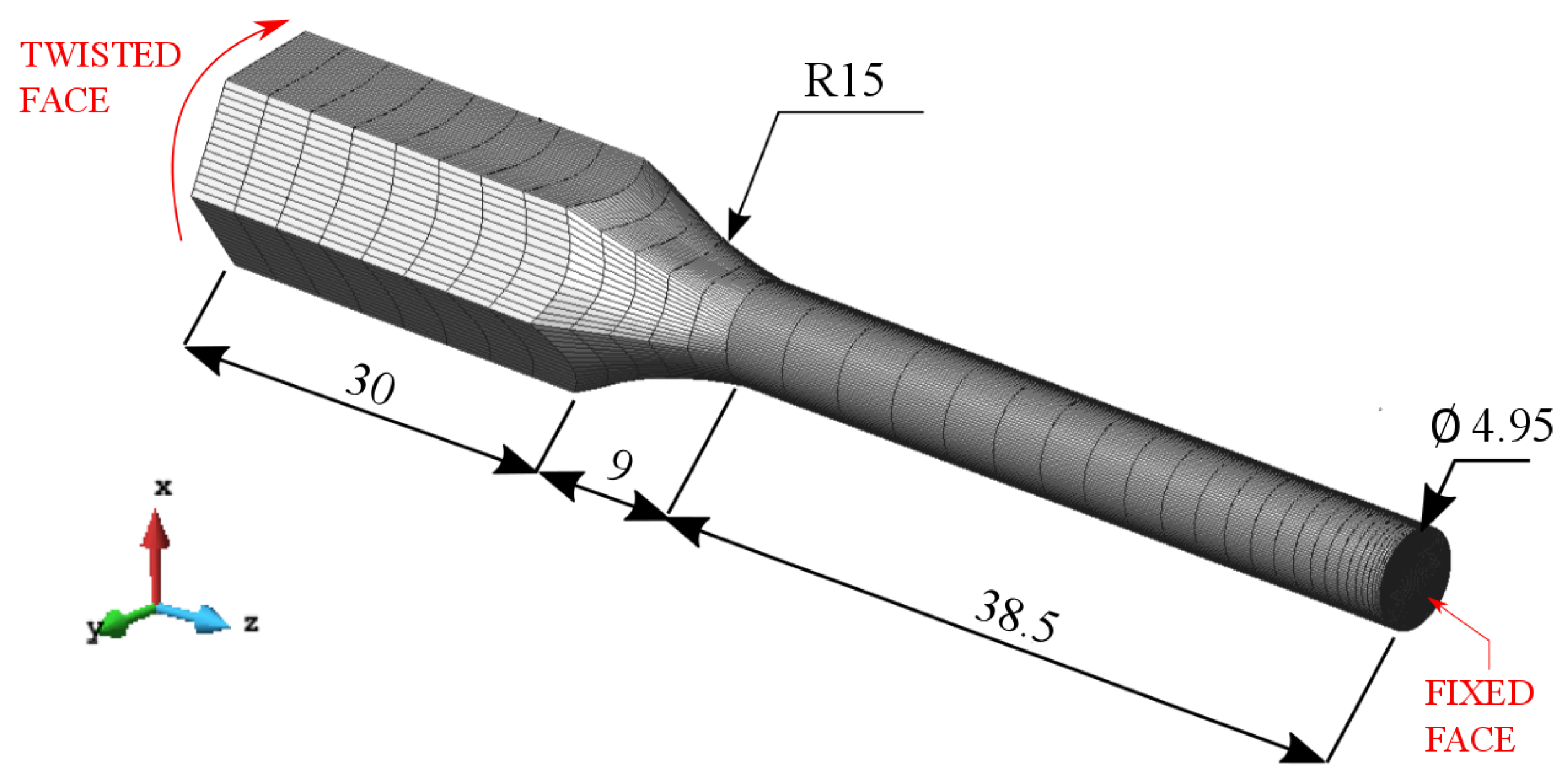
2.3.2. Torsion Test
2.4. Fitting Procedure for the Tensile Test
3. Results and Discussion
3.1. Tensile Test
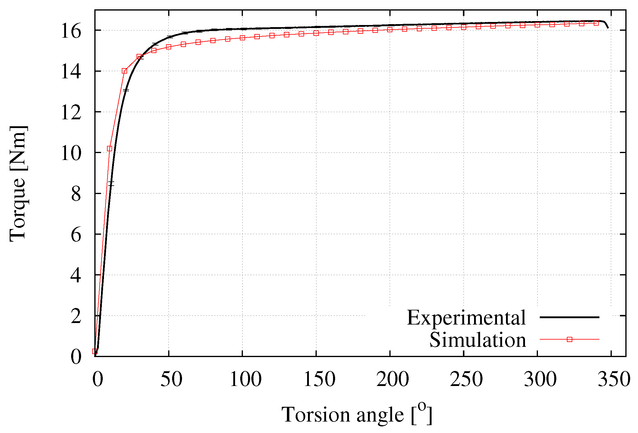
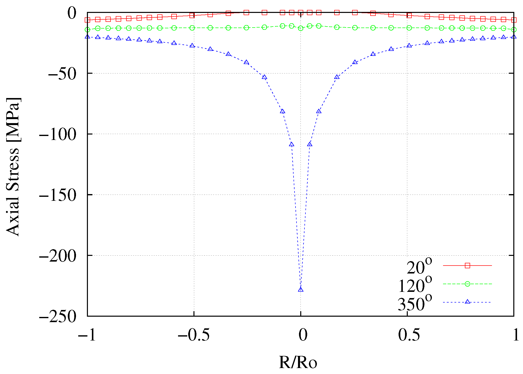
3.2. Torsion Test
4. Conclusions
Author Contributions
Funding
Acknowledgments
Conflicts of Interest
References
- Swift, W. Length changes in metals under torsional overstrain. Engineering 1947, 163, 253. [Google Scholar]
- Khoddam, S.; Beladi, H.; Hodgson, P.; Zarei-Hanzaki, A. Surface wrinkling of the twinning induced plasticity steel during the tensile and torsion tests. Mater. Des. 2014, 60, 146–152. [Google Scholar] [CrossRef]
- Khoddam, S.; Hodgson, P. Conversion of the hot torsion test results into flow curve with multiple regimes of hardening. J. Mater. Process. Technol. 2004, 153–154, 839–845. [Google Scholar] [CrossRef]
- Shrivastava, S.; Jonas, J.; Canova, G. Equivalent strain in large deformation torsion testing: Theoretical and practical considerations. J. Mech. Phys. Solids 1982, 30, 75–90. [Google Scholar] [CrossRef]
- Neale, K.W.; Shrivastava, S.C. Analytical Solutions for Circular Bars Subjected to Large Strain Plastic Torsion. J. Appl. Mech. 1990, 57, 298. [Google Scholar] [CrossRef]
- Wu, P.D.; Van der Giessen, E. Analysis of elastic-plastic torsion of circular bars at large strains. Arch. Appl. Mech. 1991, 61, 89–103. [Google Scholar] [CrossRef]
- Van der Giessen, E.; Wu, P.; Neale, K. On the effect of plastic spin on large strain elastic-plastic torsion of solid bars. Int. J. Plast. 1992, 8, 773–801. [Google Scholar] [CrossRef][Green Version]
- Zhao, H.; Zhuang, Z.; Zheng, Q. Study of Plastic Hardening-Large Deformed Torsion Test and Simulation. Key Eng. Mater. 2003, 243–244, 207–212. [Google Scholar] [CrossRef]
- Sun, L.; Zhang, M.; Hu, W.; Meng, Q. Tension-Torsion High-Cycle Fatigue Life Prediction of 2A12-T4 Aluminium Alloy by Considering the Anisotropic Damage: Model, Parameter Identification, and Numerical Implementation. Acta Mech. Solida Sin. 2016, 29, 391–406. [Google Scholar] [CrossRef]
- Yeganeh, M.; Naghdabadi, R. Axial effects investigation in fixed-end circular bars under torsion with a finite deformation model based on logarithmic strain. Int. J. Mech. Sci. 2006, 48, 75–84. [Google Scholar] [CrossRef]
- Duchêne, L.; El Houdaigui, F.; Habraken, A.M. Length changes and texture prediction during free end torsion test of copper bars with FEM and remeshing techniques. Int. J. Plast. 2007, 23, 1417–1438. [Google Scholar] [CrossRef]
- E28 Committee. Test Methods for Tension Testing of Metallic Materials; Technical Report; ASTM International: West Conshohocken, PA, USA, 2016. [Google Scholar] [CrossRef]
- Standard, A. Standard Test Method for Poisson’s Ratio at Room Temperature; E132-97; Annual Book of ASTM Standards: Philadelphia, PA, USA, 2002; Volume 3, pp. 275–277. [Google Scholar]
- Standard Test Method for Young’s Modulus, Tangent Modulus, and Chord Modulus; Reapproved in 2010; ASTM: West Conshohocken, PA, USA, 2004.
- Cabezas, E.E.; Celentano, D.J. Experimental and numerical analysis of the tensile test using sheet specimens. Finite Elem. Anal. Des. 2004, 40, 555–575. [Google Scholar] [CrossRef]
- Tao, H.; Zhang, N.; Tong, W. An iterative procedure for determining effective stress–strain curves of sheet metals. Int. J. Mech. Mater. Des. 2009, 5, 13–27. [Google Scholar] [CrossRef]
- Abeyaratne, R. Lecture Notes on The Mechanics of Elastic Solids Volume II: Continuum Mechanics; Electronic Publication: Galway, Ireland, 1952. [Google Scholar]
- Faleskog, J.; Barsoum, I. Tension-torsion fracture experiments—Part I: Experiments and a procedure to evaluate the equivalent plastic strain. Int. J. Solids Struct. 2013, 50, 4241–4257. [Google Scholar] [CrossRef]


| C [%] 0.433 | Si [%] 0.218 | Mn [%] 0.73 | P [%] 0.01 | S [%] 0.013 |
| Cr [%] 0.019 | Mo [%] 0.014 | Ni [%] 0.044 | Al [%] 0.0023 | Cu [%] 0.042 |
| Nb [%] <0.001 | Ti [%] 0.0009 | V [%] 0.0022 | W [%] <0.007 | Pb [%] <0.001 |
| Sn [%] 0.0059 | B [%] 0.0027 | Co [%] 0.0088 | Fe [%] 98.3 |
| Parameter | Value |
|---|---|
| E | 208 GPa |
| 0.271 | |
| Tensile strength | 840 MPa |
| 560 MPa | |
| 0.033 | |
| 950 MPa |
© 2019 by the authors. Licensee MDPI, Basel, Switzerland. This article is an open access article distributed under the terms and conditions of the Creative Commons Attribution (CC BY) license (http://creativecommons.org/licenses/by/4.0/).
Share and Cite
Toro, S.A.; Aranda, P.M.; García-Herrera, C.M.; Celentano, D.J. Analysis of the Elastoplastic Response in the Torsion Test Applied to a Cylindrical Sample. Materials 2019, 12, 3200. https://doi.org/10.3390/ma12193200
Toro SA, Aranda PM, García-Herrera CM, Celentano DJ. Analysis of the Elastoplastic Response in the Torsion Test Applied to a Cylindrical Sample. Materials. 2019; 12(19):3200. https://doi.org/10.3390/ma12193200
Chicago/Turabian StyleToro, Sebastián Andrés, Pedro Miguel Aranda, Claudio Moisés García-Herrera, and Diego Javier Celentano. 2019. "Analysis of the Elastoplastic Response in the Torsion Test Applied to a Cylindrical Sample" Materials 12, no. 19: 3200. https://doi.org/10.3390/ma12193200
APA StyleToro, S. A., Aranda, P. M., García-Herrera, C. M., & Celentano, D. J. (2019). Analysis of the Elastoplastic Response in the Torsion Test Applied to a Cylindrical Sample. Materials, 12(19), 3200. https://doi.org/10.3390/ma12193200