A Review of Statistical Failure Time Models with Application of a Discrete Hazard Based Model to 1Cr1Mo-0.25V Steel for Turbine Rotors and Shafts


Abstract
:1. Introduction
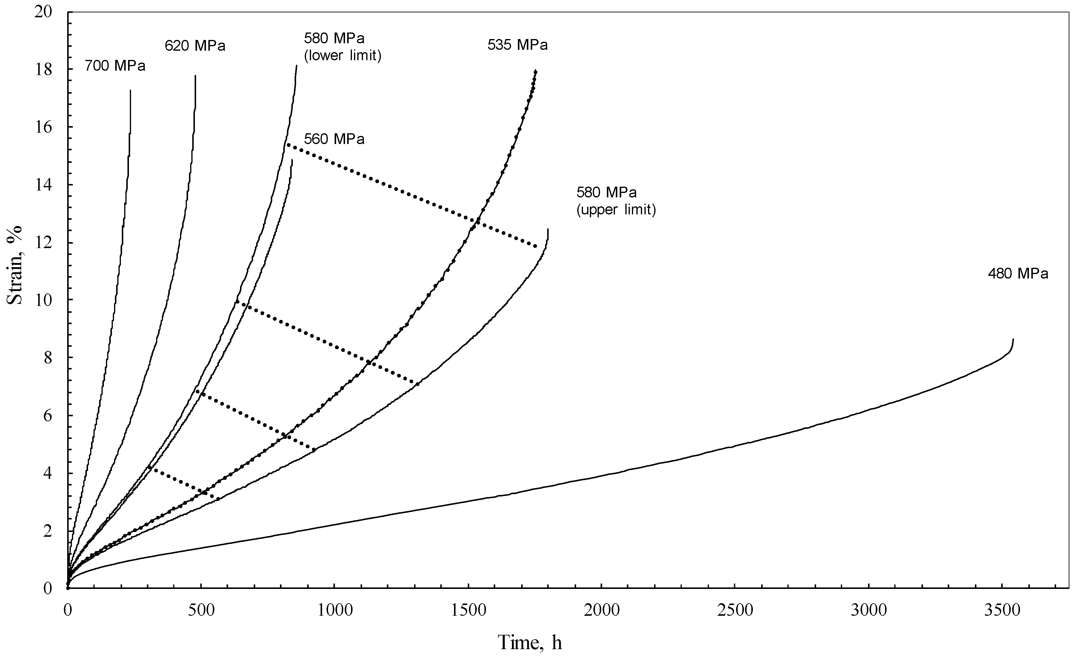
2. The Data
3. Illustrated Review of Approaches to Modelling the Stochastic Nature of Creep Failure
3.1. A Statistical Description of Continuous Failure at Fixed Test Conditions
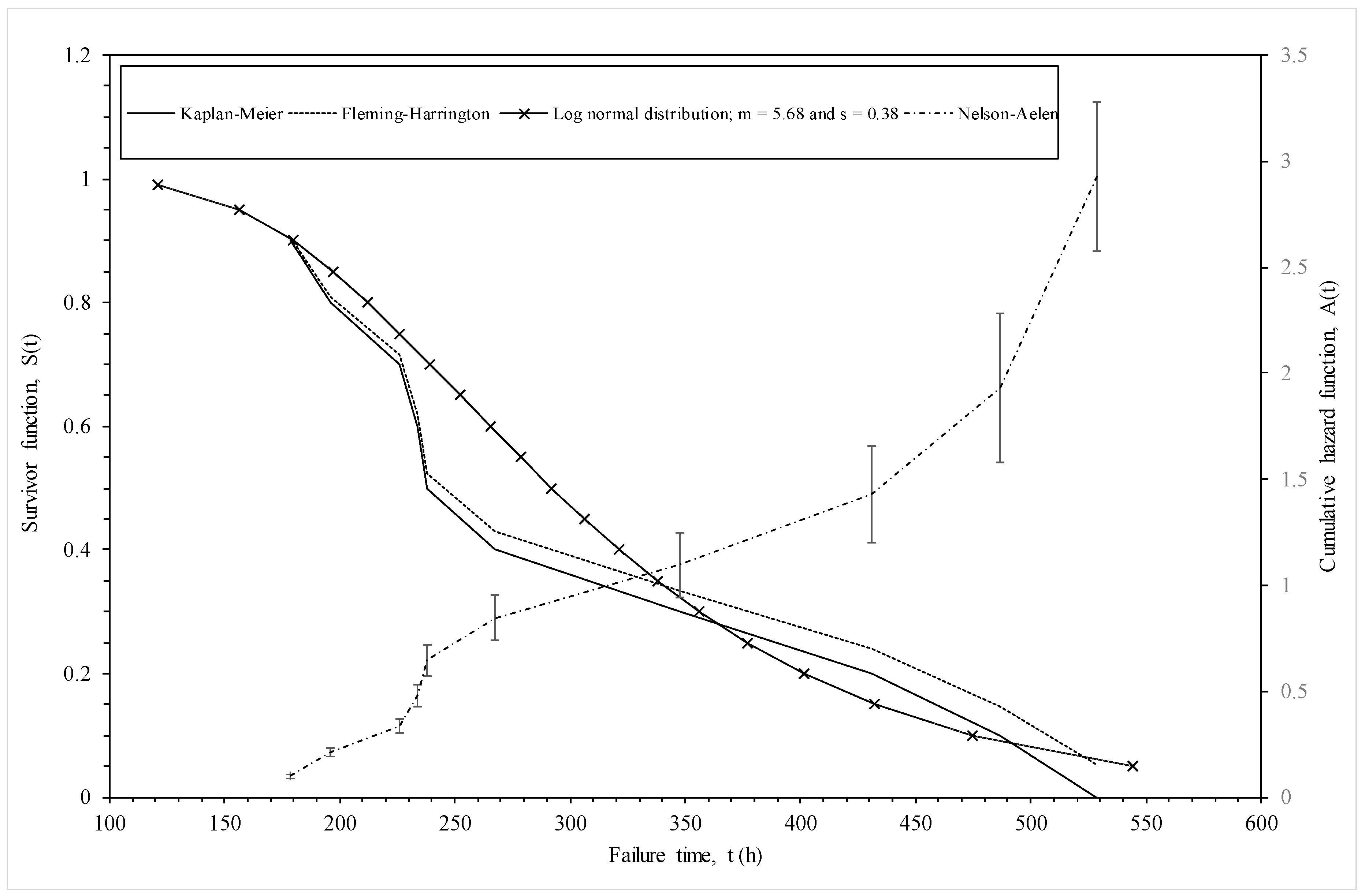
3.1.1. Non-Parametric Estimation
3.1.2. Parametric Estimation
3.2. A Statistical Description of Continuous Failure Times at Varying Test Conditions
3.2.1. Accelerated Failure Time Models (AFT)
3.2.2. Proportional Odds Models
3.2.3. Proportional Hazard Models (PH)
3.3. Modelling Discrete Failure Times at Varying Test Conditions
3.3.1. Creating Discrete Data from Continuous Data
3.3.2. Re-Specification of the Continuous Hazard Based Models
3.3.3. Estimation
3.3.4. Assessing Model Adequacy
4. Application of Discrete Hazard Function to Batch VaA of 1Cr-1Mo-0.25V
4.1. Incorporating Wilshire Variables into a Discrete Hazard Model
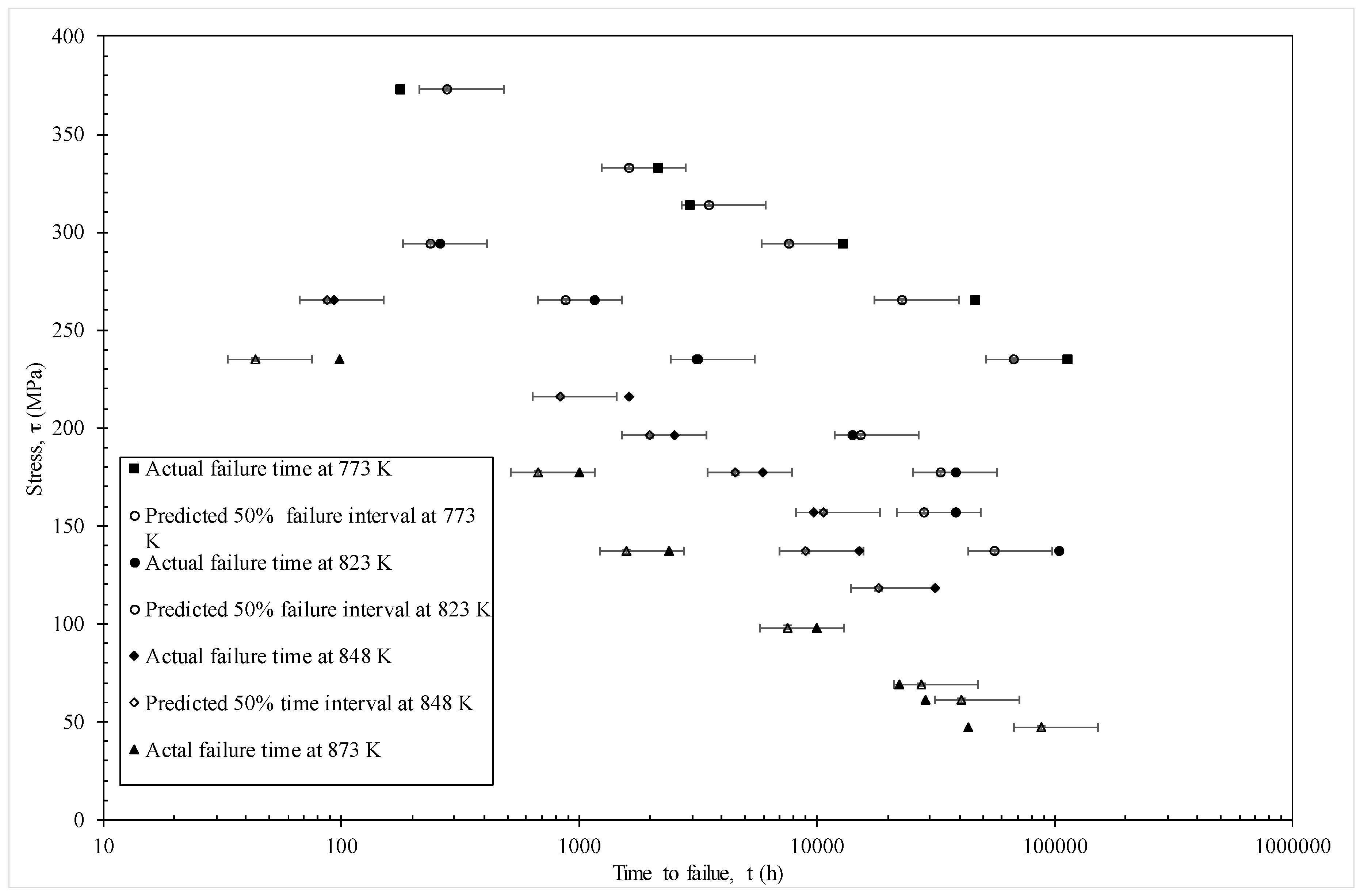
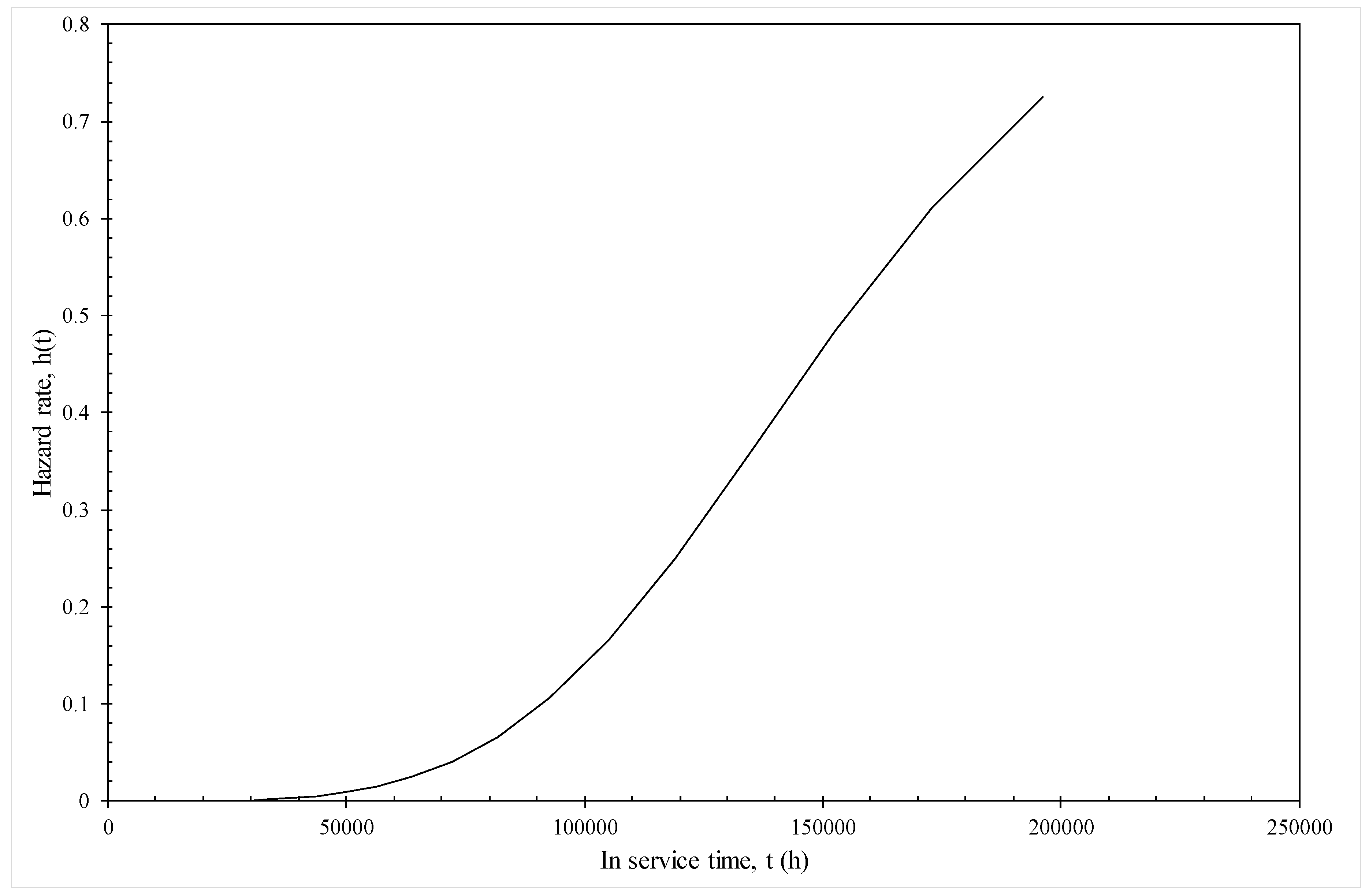
4.2. Results
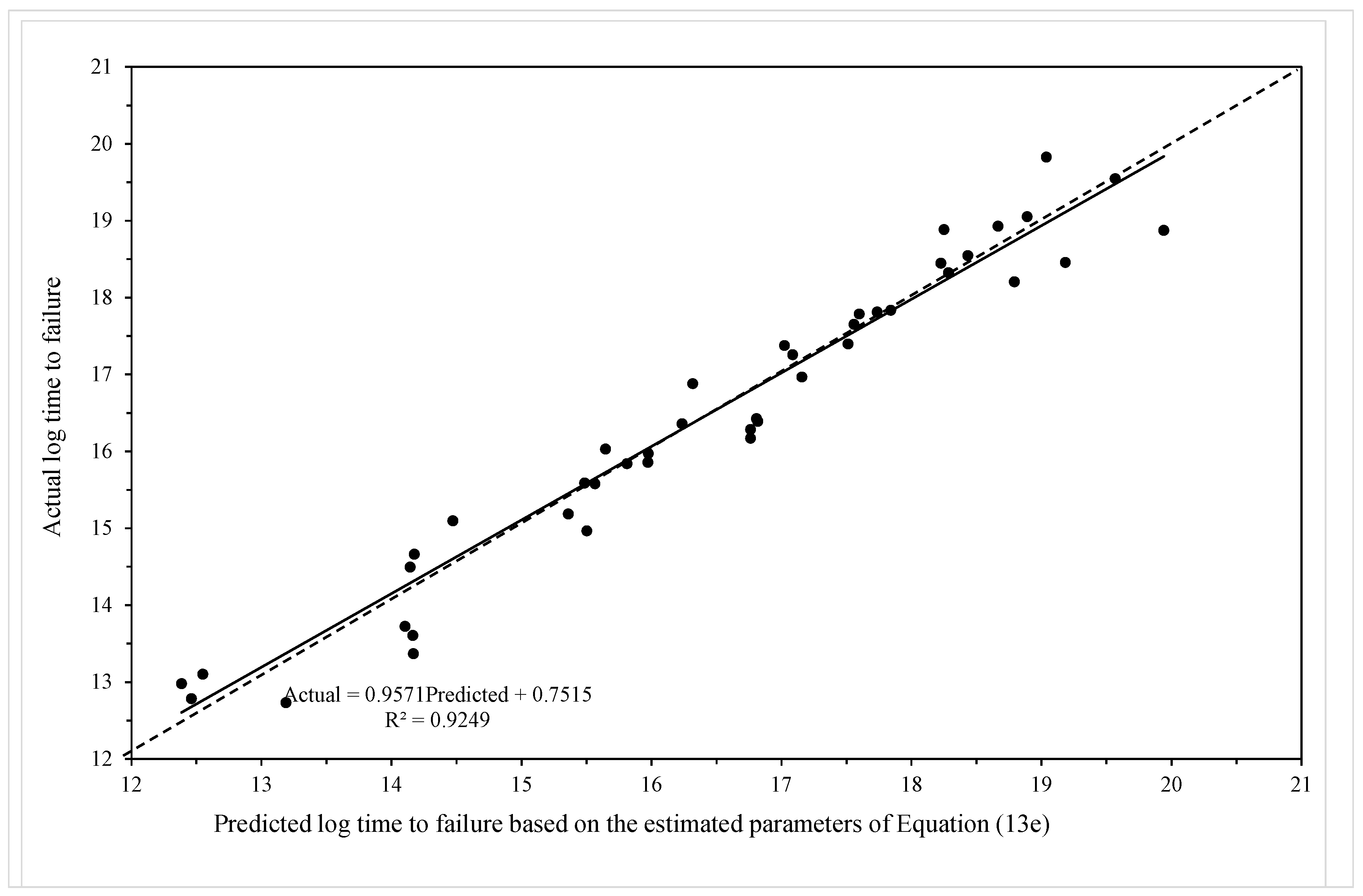
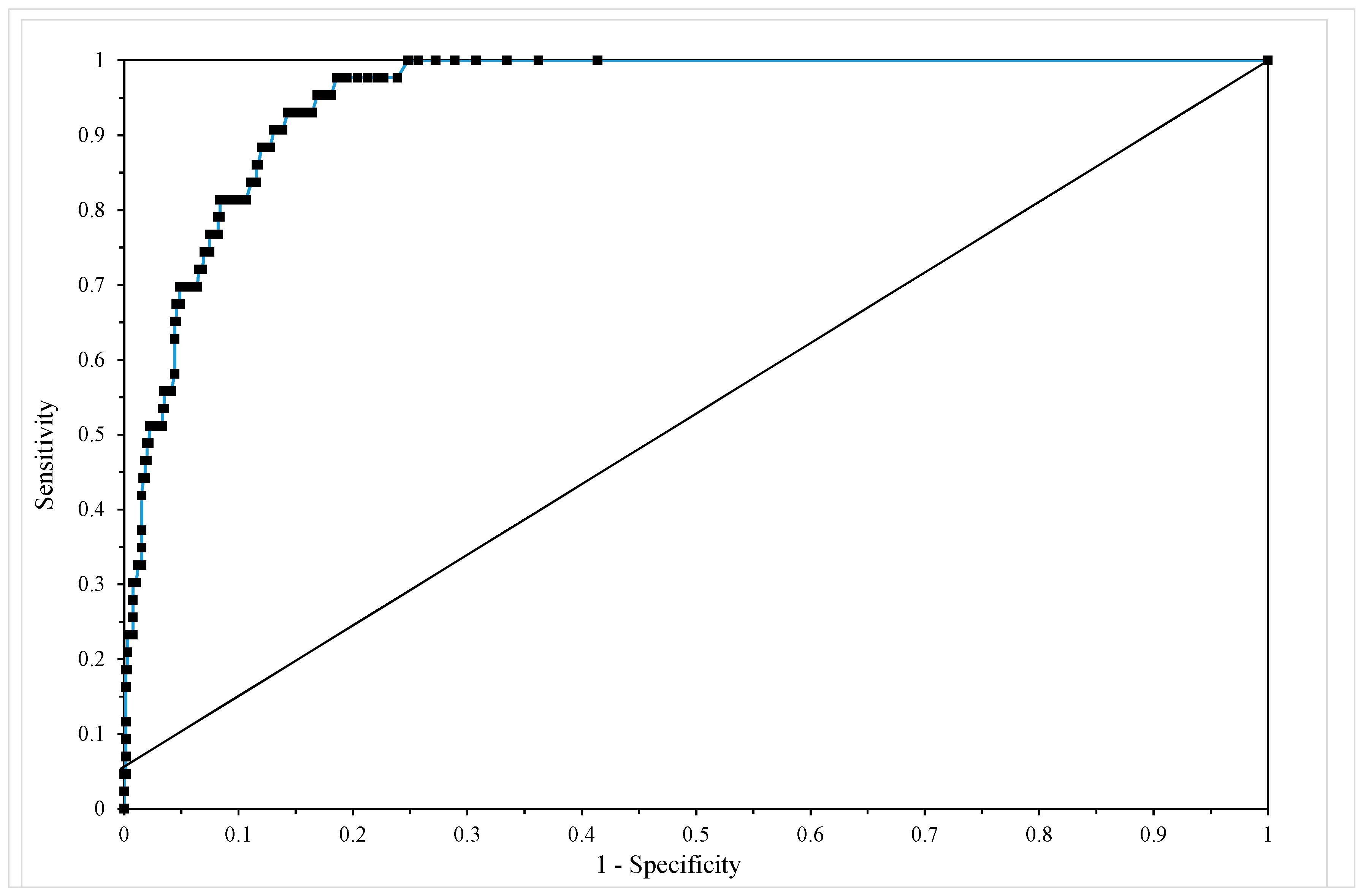
4.2.1. Model Given by Equation (19e)
4.2.2. Model Given by Equation (19f)
5. Conclusions
Conflicts of Interest
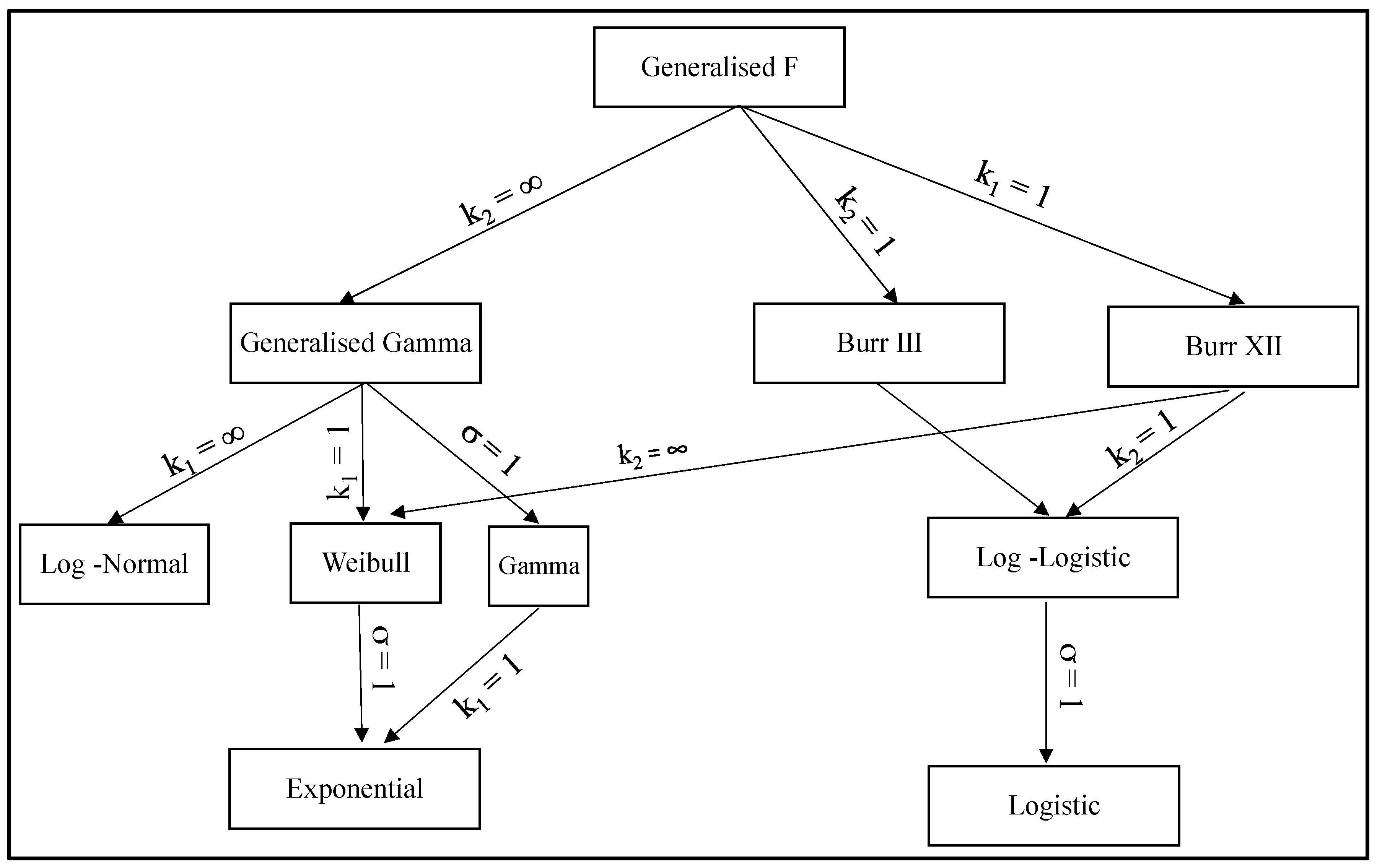
Appendix A. The Generalised F Family of Failure Time Distributions
Appendix A.1. The Generalized Logistic Family
Appendix A.1.1. The Burr XII [46] Distribution (k1 = 1)
Appendix A.1.2. The Burr III Distribution (k2 = 1)
Appendix A.1.3. The Log-Logistic [47] Distribution (k1 = k2 = 1)
Appendix A.1.4. The Logistic Distribution (k1 = k2 = σ = 1)
Appendix A.2. The Generalised Gamma Family
Appendix A.2.1. The Generalised Gamma Distribution (k2 = ∞)
Appendix A.2.2. The Weibull (k1 = 1) [49] and Exponential Distributions (k1 = 1 = σ)
Appendix A.2.3. The Gamma [50] Distribution (σ = 1).
Appendix A.2.4. The Log Normal Distribution (k1 = k2 = ∞)
References
- Allen, D.; Garwood, S. Energy Materials-Strategic Research Agenda. Q2. Materials Energy Review; IoMMh: London, UK, 2007. [Google Scholar]
- Evans, R.W.; Wilshire, B. Creep of Metals and Alloys; The Institute of Metals: London, UK, 1985. [Google Scholar]
- Evans, R.W. A Constitutive Model for the High Temperature Creep of Particle-hardened Alloys on the Θ Projection Method. Proc. R. Soc. 1996, A456, 835–868. [Google Scholar] [CrossRef]
- McVetty, P.G. Creep of Metals at Elevated Temperatures—The Hyperbolic Sine Relation between Stress and Creep Rate. Trans. ASME 1943, 65, 761–769. [Google Scholar]
- Garofalo, F. Fundamentals of Creep Rupture in Metals; Macmillan: New York, NY, USA, 1965. [Google Scholar]
- Ion, J.C.; Barbosa, A.; Ashby, M.F.; Dyson, B.F.; McLean, M. The Modelling of Creep for Engineering Design. I; NPL Report DMA A115; National Physical Laboratory: London, UK, April 1986. [Google Scholar]
- Prager, M. The Omega Method- An Engineering Approach to Life Assessment. J. Press. Vessel. Technol. 2000, 22, 273–280. [Google Scholar] [CrossRef]
- Othman, A.M.; Hayhurst, D.R. Multi-Axial Creep Rupture of a Model Structure using a Two Parameter Material Model. Int. J. Mech. Sci. 1990, 32, 35–48. [Google Scholar] [CrossRef]
- Kachanov, L.M. The Theory of Creep; Kennedy, A.J., Ed.; National Lending Library: Boston, UK, 1967. [Google Scholar]
- Rabotnov, Y.N. Creep Problems in Structural Members; North-Holland: Amsterdam, The Netherlands, 1969. [Google Scholar]
- Monkman, F.C.; Grant, N.J. An Empirical Relationship between Rupture Life and Minimum Creep Rate. In Deformation and Fracture at Elevated Temperature; Grant, N.J., Mullendore, A.W., Eds.; MIT Press: Boston, MA, USA, 1963. [Google Scholar]
- Dorn, J.E.; Shepherd, L.A. What We Need to Know About Creep. In Proceedings of the STP 165 Symposium on The Effect of Cyclical Heating and Stressing on Metals at Elevated Temperatures, Chicago, IL, USA, 17 June 1954. [Google Scholar]
- Larson, F.R.; Miller, J. A Time Temperature Relationship for Rupture and Creep Stresses. Trans. ASME 1952, 174, 5. [Google Scholar]
- Manson, S.S.; Haferd, A.M. A Linear Time-Temperature Relation for Extrapolation of Creep and Stress-Rupture Data; NACA Technical Note 2890; National Advisory Committee for Aeronautics: Cleveland, OH, USA, 1953.
- Manson, S.S.; Muraldihan, U. Analysis of Creep Rupture Data in Five Multi Heat Alloys by Minimum Commitment Method Using Double Heat Term Centring Techniques; Progress in Analysis of Fatigue and Stress Rupture MPC-23; ASME: New York, NY, USA, 1983; pp. 1–46. [Google Scholar]
- Manson, S.S.; Brown, W.F.J. Time-Temperature-Stress Relations for the Correlation and Extrapolation of Stress Rupture Data. Proc. ASTM 1953, 53, 693–719. [Google Scholar]
- Trunin, I.I.; Golobova, N.G.; Loginov, E.A. New Methods of Extrapolation of Creep Test and Long Time Strength Results. In Proceedings of the 4th International Symposium on Heat Resistant Metallic Materials, Mala Fatra, Czechoslovakia, 1971. [Google Scholar]
- Abdallah, Z.; Perkins, K.; Whittaker, M. A Critical Analysis of the Conventionally Employed Creep Lifing Methods. Materials 2014, 7, 3371–3398. [Google Scholar] [CrossRef] [PubMed]
- Williams, S.J. An Automatic Technique for the Analysis of Stress Rupture Data; Report MFR30017; Rolls-Royce Plc: Derby, UK, 1993. [Google Scholar]
- Wilshire, B.; Battenbough, A.J. Creep and Creep Fracture of Polycrystalline Copper. Mater. Sci. Eng. A 2007, 443, 156–166. [Google Scholar] [CrossRef]
- Wilshire, B.; Scharning, P.J. Prediction of Long Term Creep Data for Forged 1Cr-1Mo-0.25V Steel. Mater. Sci. Technol. 2008, 24, 1–9. [Google Scholar] [CrossRef]
- Wilshire, B.; Whittaker, M. Long Term Creep Life Prediction for Grade 22 (2·25Cr-1Mo) Steels. Mater. Sci. Technol. 2011, 27, 642–647. [Google Scholar]
- Wilshire, B.; Scharning, P.J. A New Methodology for Analysis of Creep and Creep Fracture Data for 9–12% Chromium Steels. Int. Mater. Rev. 2008, 53, 91–104. [Google Scholar] [CrossRef]
- Abdallah, A.; Perkins, K.; Williams, S. Advances in the Wilshire Extrapolation Technique—Full Creep Curve Representation for the Aerospace Alloy Titanium 834. Mater. Sci. Eng. A 2012, 550, 176–182. [Google Scholar] [CrossRef]
- Whittaker, M.T.; Evans, M.; Wilshire, B. Long-Term Creep Data Prediction for Type 316H Stainless Steel. Mater. Sci. Eng. A 2012, 552, 145–150. [Google Scholar] [CrossRef]
- Evans, M. Incorporating specific batch characteristics such as chemistry, heat treatment, hardness and grain size into the Wilshire equations for safe life prediction in high temperature applications: An application to 12Cr stainless steel bars for turbine blades. Appl. Math. Model. 2016, 40, 10342–10359. [Google Scholar] [CrossRef]
- Zieliński, A.; Golański, G.; Sroka, M. Comparing the Methods in Determining Residual Life on the Basis of Creep Tests of Low-Alloy Cr-Mo-V Cast Steels Operated Beyond the Design Service Life. Int. J. Press. Vess. Pip. 2017, 152, 1–6. [Google Scholar]
- Sroka, M.; Zieliński, A.; Dziuba-Kałuża, M.; Kremzer, M.; Macek, M.; Jasiński, A. Assessment of the Residual Life of Steam Pipeline Material beyond the Computational Working Time. Metals 2017, 7, 82. [Google Scholar] [CrossRef]
- Evans, R.W.; Evans, M. Numerical Modelling the Small Disc Creep Test. J. Mater. Sci. Technol. 2006, 22, 1155–1162. [Google Scholar] [CrossRef]
- NIMS Creep Data Sheet No. 9b, 1990. Available online: http://smds.nims.go.jp/MSDS/en/sheet/Creep.html (accessed on 1 April 2017).
- Evans, M. A stochastic Lifing Method for Materials Operating under Long Service Conditions: With Application to the Creep Life of a Commercial Titanium Alloy. J. Mater. Sci. 2001, 36, 4927–4941. [Google Scholar] [CrossRef]
- Evans, M. A Re-evaluation of the Causes of Deformation in 1Cr1Mo-0.25V Steel for Turbine Rotors and Shafts based on iso-Thermal Plots of the Wilshire Equation and the Modelling of Batch to Batch Variation. Materials 2017, 10, 575. [Google Scholar] [CrossRef] [PubMed]
- Kaplan, E.L.; Meier, P. Nonparametric Estimation from Incomplete Observations. J. Am. Stat. Assoc. 1958, 53, 457–481. [Google Scholar] [CrossRef]
- Nelson, W. Theory and Applications of Hazard Plotting for Censored Failure Data. Technometrics 1972, 14, 945–965. [Google Scholar] [CrossRef]
- Aalen, O.O. Nonparametric Inference for a Family of Counting Processes. Ann. Stat. 1978, 6, 701–726. [Google Scholar] [CrossRef]
- Fleming, T.R.; Harrington, D.P. Counting Processes and Survival Analysis; Wiley: New York, NY, USA, 1991. [Google Scholar]
- Prentice, R.L. Discrimination amongst Some Parametric Models. Biometrika 1975, 62, 607–614. [Google Scholar] [CrossRef]
- Kalbfleisch, J.D.; Prentice, R.L. The Statistical Analysis of Failure Time Data, 2nd ed.; Wiley: New York, NJ, USA, 2002; Chapter 3. [Google Scholar]
- Cox, D.R. Regression Models and Life-Tables. J. R. Stat. Soc. Ser. B 1972, 34, 187–220. [Google Scholar]
- Singer, J.D.; Willett, J.B. Applied Longitudinal Data Analysis: Modelling Change and Event Occurrence; Oxford University Press: New York, NY, USA, 2003. [Google Scholar]
- Berndt, B.; Hall, B.; Hall, R.; Hausman, J. Estimation and Inference in Nonlinear Structural Models. Ann. Econ. Soc. Meas. 1974, 3, 653–665. [Google Scholar]
- McCullagh, P.; Nelder, J. Generalized Linear Models, 2nd ed.; Chapman and Hall/CRC: Boca Raton, FL, USA, 1989; Chapter 2. [Google Scholar]
- Hosmer, D.W.; Lemeshow, S. Applied Logistic Regression; Wiley: New York, NY, USA, 2013. [Google Scholar]
- Abramowitz, M.; Stegun, I.A. Handbook of Mathematical Functions with Formulas, Graphs, and Mathematical Tables; Dover Publications: New York, NY, USA, 1964. [Google Scholar]
- William, W.Q.; Escobar, L.A. Statistical Methods for Reliability Data; John Wiley & Sons: New York, NY, USA, 1998; Chapters 4 and 5. [Google Scholar]
- Burr, I.W. Cumulative Frequency Functions. Ann. Math. Stat. 1942, 13, 215–232. [Google Scholar] [CrossRef]
- Bennett, S. Log-Logistic Regression Models for Survival Data. J. R. Stat. Soc. Ser. C 1983, 32, 165–171. [Google Scholar] [CrossRef]
- Gumbel, E.J. The Return Period of Flood Flows. Ann. Math. Stat. 1941, 12, 163–190. [Google Scholar] [CrossRef]
- Weibull, W. A Statistical Distribution Function of wide Applicability. J. Appl. Mech. Trans. ASME 1951, 18, 293–297. [Google Scholar]
- Choi, S.C.; Wette, R. Maximum Likelihood Estimation of the Parameters of the Gamma Distribution and Their Bias. Technometrics 1969, 11, 683–690. [Google Scholar] [CrossRef]
- Lawless, J.F. Statistical Models and Methods for Lifetime Data, 2nd ed.; Wiley: Hoboken, NJ, USA, 2003; Chapter 1. [Google Scholar]


| Time Interval Ij = aj−1 − aj (Log Seconds) | Specimen Number, i | Stress, x1 (MPa) | Temperature, x2 (K) | vij |
|---|---|---|---|---|
| 12.5–13.0 | 1 | 412 | 723 | 0 |
| 13.0–13.5 | 1 | 412 | 723 | 0 |
| 13.5–14.0 | 1 | 412 | 723 | 0 |
| 14.0–14.5 | 1 | 412 | 723 | 0 |
| 14.5–15.0 | 1 | 412 | 723 | 0 |
| 15.0–15.5 | 1 | 412 | 723 | 0 |
| 15.5–16.0 | 1 | 412 | 723 | 0 |
| 16.0–16.5 | 1 | 412 | 723 | 1 |
| 12.5–13.0 | 2 | 373 | 723 | 0 |
| 13.0–13.5 | 2 | 373 | 723 | 0 |
| 13.5–14.0 | 2 | 373 | 723 | 0 |
| 14.0–14.5 | 2 | 373 | 723 | 0 |
| 14.5–15.0 | 2 | 373 | 723 | 0 |
| 15.0– 15.5 | 2 | 373 | 723 | 0 |
| 15.5–16.0 | 2 | 373 | 723 | 0 |
| 16.0–16.5 | 2 | 373 | 723 | 0 |
| 16.5–17.0 | 2 | 373 | 723 | 0 |
| 17.0–17.5 | 2 | 373 | 723 | 0 |
| 17.5–18.0 | 2 | 373 | 723 | 1 |
| Predicted vij | Observed vij | Total | |
|---|---|---|---|
| Survived: vij = 0 | Failed: vij = 1 | ||
| Survived: vij = 0 | m1 | m3 | M3 |
| Failed: vij = 1 | m2 | m4 | M4 |
| Total | M1 | M2 | M |
| Parameter | Variable | Estimate | Student t-value |
|---|---|---|---|
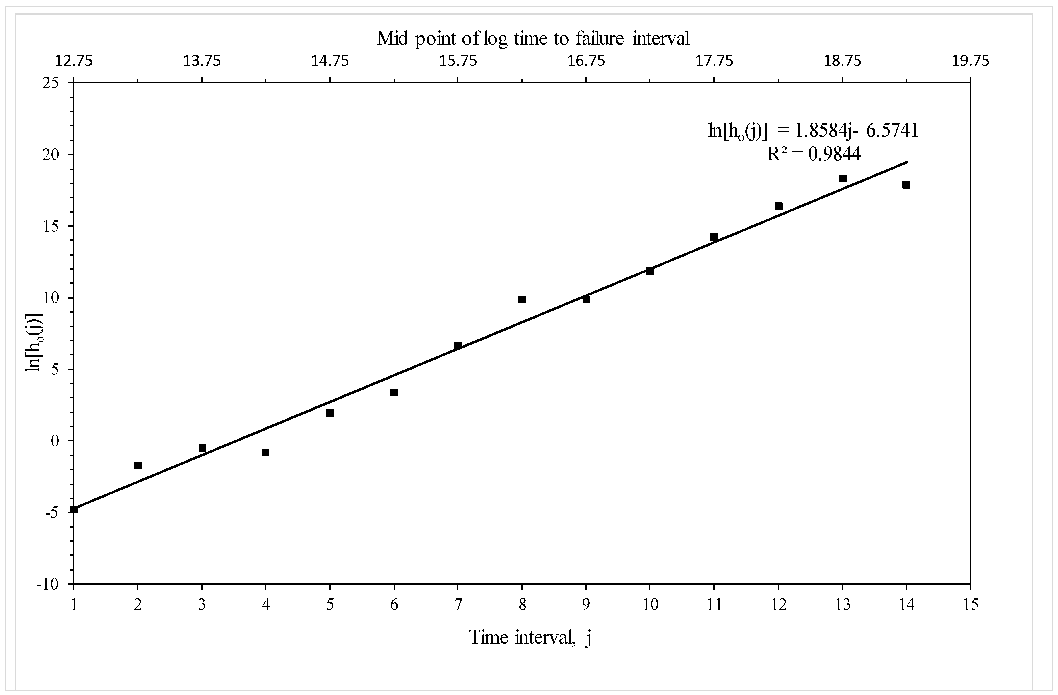
| b0,1 | ln[ho(j = 1)] for 12.5–13.0 | −4.7526 | −2.81 ** |
| b0,2 | ln[ho(j = 2)] for 13.0–13.5 | −1.7111 | −1.43 |
| b0,3 | ln[ho(j = 3)] for 13.5–14.0 | −0.5019 | −0.48 |
| b0,4 | ln[ho(j = 4)] for 14.0–14.5 | −0.7838 | −0.53 |
| b0,5 | ln[ho(j = 5)] for 14.5–15.0 | 1.9713 | 1.26 |
| b0,6 | ln[ho(j = 6)] for 15.0–15.5 | 3.4266 | 2.16 ** |
| b0,7 | ln[ho(j = 7)] for 15.5–16.0 | 6.7247 | 4.24 *** |
| b0,8 | ln[ho(j = 8)] for 16.0–16.5 | 9.8840 | 4.81 *** |
| b0,9 | ln[ho(j = 9)] for 16.5–17.0 | 9.9378 | 4.31 *** |
| b0,10 | ln[ho(j = 10)] for 17.0–17.5 | 11.9647 | 4.85 *** |
| b0,11 | ln[ho(j = 11)] for 17.5–18.0 | 14.2367 | 5.11 *** |
| b0,12 | ln[ho(j = 12)] for 18.0–18.5 | 16.4289 | 5.27 *** |
| b0,13 | ln[ho(j = 13)] for 18.5–19.0 | 18.3696 | 5.39 *** |
| b0,14 | ln[ho(j = 14)] for 19.0–19.5 | 17.9018 | 5.04 *** |
| b0,15 | ln[ho(j = 15)] for 19.5–20.0 | 19.2411 | 0.38 |
| b1 | x1 | −28.554 | −5.13 *** |
| b2 | x2 | −1363.8818 | −5.62 *** |
| b3 | x3 | 5.4672 | 2.37 ** |
| b4 | x4 | 642.0808 | −4.43 *** |
| Predicted vij | Observed vij | Total | |
|---|---|---|---|
| Survived: vij = 0 | Failed: vij = 1 | ||
| Survived: vij = 0 | 306 | 14 | 320 |
| Failed: vij = 1 | 9 | 29 | 38 |
| Total | 315 | 43 | 358 |
| Parameter | Variable | Estimate | Student t-value |
|---|---|---|---|
| a | Constant | −5.8351 | −4.91 *** |
| b0 | Time trend, j | 2.0736 | 6.02 *** |
| b1 | x1 | −30.8703 | −5.85 *** |
| b2 | x2 | −1451.7496 | −5.93 *** |
| b3 | x3 | 5.1666 | 3.84 *** |
| b4 | x4 | 596.9284 | 4.48 *** |
| Predicted vij | Observed vij | Total | |
|---|---|---|---|
| Survived: vij = 0 | Failed: vij = 1 | ||
| Survived: vij = 0 | 305 | 13 | 318 |
| Failed: vij = 1 | 10 | 30 | 40 |
| Total | 315 | 43 | 358 |
© 2017 by the author. Licensee MDPI, Basel, Switzerland. This article is an open access article distributed under the terms and conditions of the Creative Commons Attribution (CC BY) license (http://creativecommons.org/licenses/by/4.0/).
Share and Cite
Evans, M. A Review of Statistical Failure Time Models with Application of a Discrete Hazard Based Model to 1Cr1Mo-0.25V Steel for Turbine Rotors and Shafts. Materials 2017, 10, 1190. https://doi.org/10.3390/ma10101190
Evans M. A Review of Statistical Failure Time Models with Application of a Discrete Hazard Based Model to 1Cr1Mo-0.25V Steel for Turbine Rotors and Shafts. Materials. 2017; 10(10):1190. https://doi.org/10.3390/ma10101190
Chicago/Turabian StyleEvans, Mark. 2017. "A Review of Statistical Failure Time Models with Application of a Discrete Hazard Based Model to 1Cr1Mo-0.25V Steel for Turbine Rotors and Shafts" Materials 10, no. 10: 1190. https://doi.org/10.3390/ma10101190
APA StyleEvans, M. (2017). A Review of Statistical Failure Time Models with Application of a Discrete Hazard Based Model to 1Cr1Mo-0.25V Steel for Turbine Rotors and Shafts. Materials, 10(10), 1190. https://doi.org/10.3390/ma10101190