Energy and Environmental Efficiency for the N-Ammonia Removal Process in Wastewater Treatment Plants by Means of Reinforcement Learning

Abstract

Currently, energy and environmental efficiency are critical aspects in wastewater treatment plants (WWTPs). In fact, WWTPs are significant energy consumers, especially in the active sludge process (ASP) for the N-ammonia removal. In this paper, we face the challenge of simultaneously improving the economic and environmental performance by using a reinforcement learning approach. This approach improves the costs of the N-ammonia removal process in the extended WWTP Benchmark Simulation Model 1 (BSM1). It also performs better than a manual plant operator when disturbances affect the plant. Satisfactory experimental results show significant savings in a year of a working BSM1 plant.

1. Introduction

The main objective of wastewater treatment is to provide humans and industries mechanisms for disposing effluents to protect the natural environment.

In recent years, many efforts are being globally conducted to assess these environmental problems [1,2,3]. A growing number of organizations research ways of helping the wastewater industry to meet regulatory standards, and they concern environmental sustainability [4]. It is known that governments are now more concerned about wise water use. For this reason, they are promoting specific education programs, legislation and pricing oriented both toward individuals and companies. Additionally, industries are developing new strategies to achieve better water quality while reducing the use of contaminants.

All of this implies continuous changes in regulations and standards, in order to achieve more restrictive requirements and, at the same time, to save energy. There are different reports showing the best practices for the energy-efficient operation of the wastewater industry [5,6,7], and there are also reports showing increased spending by governments in this area [8]. One of the major environmental impact factors related to wastewater treatment plants (WWTPs) has to do with their efficiency. WWTPs are significant energy consumers. From an economic point of view, it is of best interest to find efficiencies in the energy use in order to cut operating costs while rising to the challenges of water quality, sustainable development and even stringent regulations. Thus, if a WWTP is efficient in terms of energy consumption, it will be environmentally efficient. In other words, it will improve the water quality while reducing operational cost and effluent fines. Energy and environmental efficiency in WWTPs in terms of lowing energy consumption have been previously considered in the literature [9,10,11].

In the WWTPs, one of these strict regulations has been imposed on the nitrogen levels at the effluent. In this way, the active sludge process (ASP) with nitrification/denitrification stages is the most widely-used technique for biological treatment in [12]. Several variables are manipulated in WWTPs in order to control ASP [13,14]: dissolved oxygen concentration, ammonia concentration, internal recycle flowrate, sludge recycle flowrate or external carbon dosing.

Nevertheless, the variable most widely used in many plants is the dissolved oxygen (DO) concentration [14]. It is used for controlling the ASP, as the DO level in the aerobic reactors has a direct influence on the microorganisms’ activity, which are part of the active sludge. Aeration mechanisms supply oxygen to the sludge, so that organic matter is degraded and the nitrogen concentration is lowered. Thus, this makes it necessary to keep a proper concentration of DO.

Often, in many plants, the DO concentration is kept high enough to ensure good effluent quality. However, this approach is expensive, and it is therefore desired to operate the aerobic reactors of the plant at lower DO concentrations to reduce energy consumption. Notice that the process for the N-ammonia removal is the most important energy consumer in a WWTP, being responsible for near 50% of the energy consumption of the plant.

In this framework, the objective of the paper is, on the one hand, to satisfy the effluent requirements defined by local regulations to keep the total nitrogen under a limit [15,16] and, on the other hand, to keep maintenance expenses as low as possible. These expenses are due to the disposal of the wasted sludge [17,18] and mainly due to the energy consumed by blowers (for aeration) and pumps.

Optimization efforts in WWTP are focused on: (i) improving the water quality by minimizing the operational costs [19]; and (ii) minimizing the sludge production for disposal [20]. Our approach mainly deals with the first objective.

Several control strategies have been proposed to control DO concentration. Methods based on PID controllers have been widely used [21]. In general, model-based predictive control [14,22,23] and nonlinear predictive strategies [9,24] have been applied to control DO concentration in WWTPs.

Nevertheless, these methods do not always behave as they should when the quality of the influent changes in load or flow. In the control loops, optimal set-points are hard to set due to disturbances acting over the plant. Currently, these settings are manually operated by plant operators. In fact, it is required to have a somewhat intelligent control that changes the set-points of these controllers to adapt the plant to disturbances, such as the external weather conditions.

Approaches that provide more intelligent control in WWTPs have been proposed in the literature. For example, machine learning models [25,26], genetic algorithms [27] or neural networks [28,29].

Reinforcement learning (RL) has been already successfully applied to the control process in WWTPs [30]. In particular, in [30], a model-free learning control has been proposed to regulate the oxidation-reduction potential and pH neutralization in advanced oxidation processes. The point of the approach presented in [30] is to stabilize the process.

In this work, we describe a related approach to control a WWTP with a model-free RL agent focusing on efficiency instead of stability. In this case, the agent learns to change the DO set-points of the plant in an autonomous way (without a direct intervention of the plant operator). The efficiency achieved by this RL agent is measured by an operation cost (OC) that quantifies both the energy and the environmental costs. This OC is measured in euros, and the point in this paper is the optimization of the OC. In order to show the agent’s behavior, we use the Benchmark Simulation Model No. 1 (BSM1) [31]. This benchmark is intended to be a representative model of a generic WWTP.

This paper is organized as follows. Section 2, describes the BSM1 and the performance assessment. Section 3 presents the reinforcement learning approach and the WWTP simulator. Section 4 follows by presenting some experiments comparing the plant operator with the RL agent. Finally, the conclusions are presented in Section 5.

2. Working Scenario

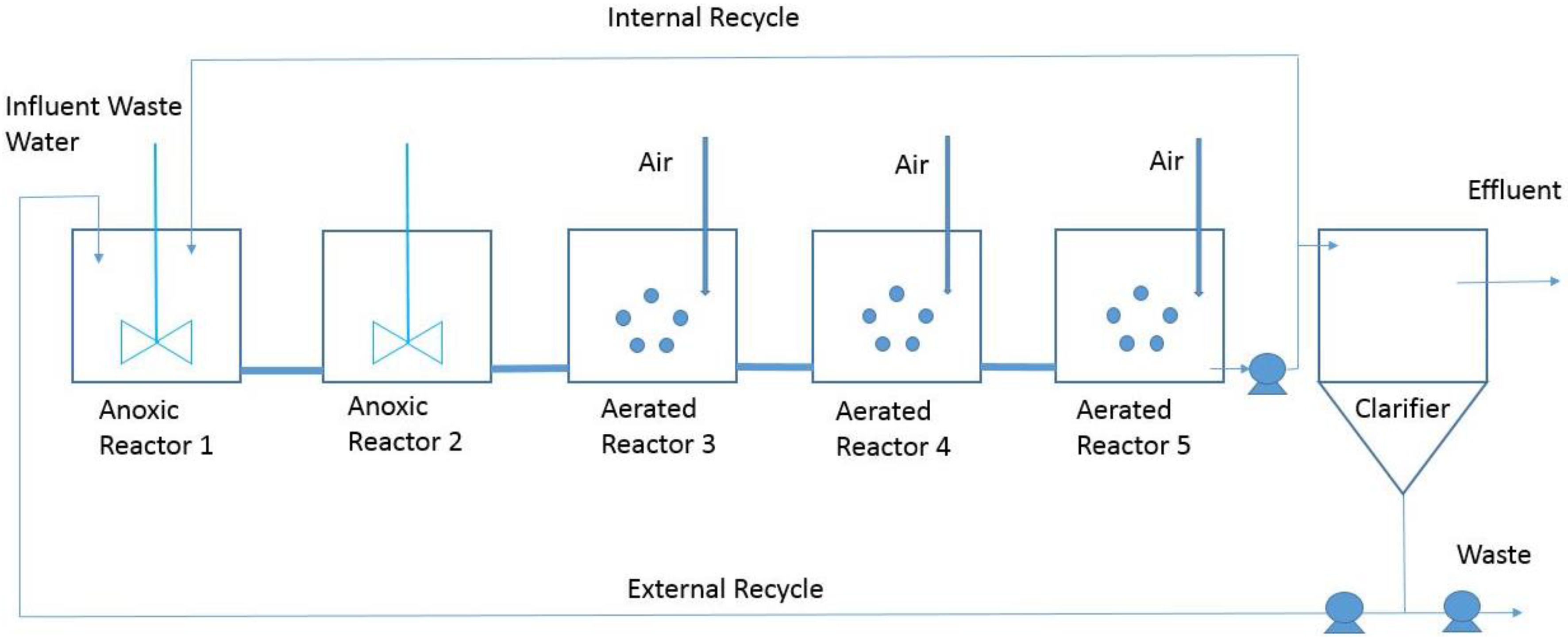
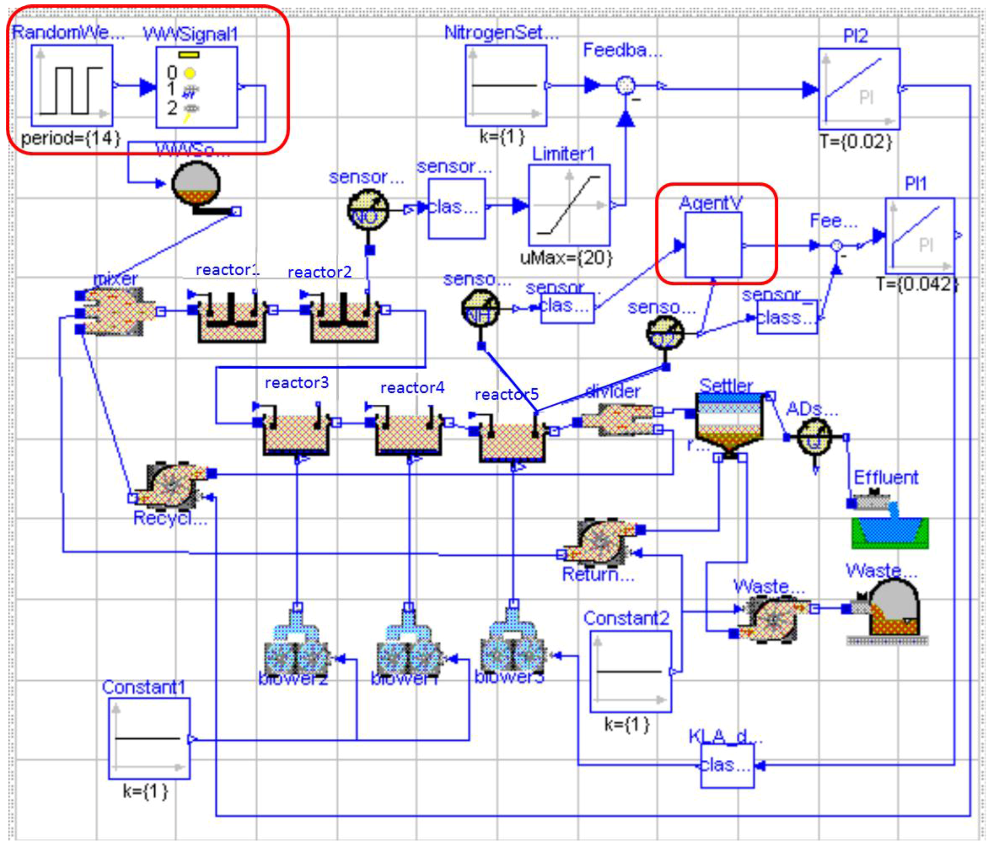
2.1. The BSM1

The Benchmark Simulation Model No. 1 or BSM1 [32] has a common layout for the full-scale current WWTP. This benchmark is an environment for the simulation of a WWTP, which defines a plant layout, a simulation model, influent loads, test procedures and evaluation criteria.

A schematic representation of the benchmark configuration is presented in Figure 1.

The plant layout aims at carbon and nitrogen removal in a series of five activated sludge reactors followed by a secondary settling tank. The first two reactors are anoxic, and the last three are aerated.

The biological phenomena taking place in the reactors (nitrogen and carbon removal processes) are modeled according to the Activated Sludge Model No. 1 (ASM1) [18], the biological parameter values used being those that correspond to a temperature of 15 °C. The ASM1 has thirteen state variables and eight dynamic processes, and it consists of a set of ordinary differential equations, which describe the dynamic changes of the state variables. The chosen secondary settler model is a one-dimensional 10-layer non-reactive unit (i.e., no biological reaction) of constant thickness with the double-exponential settling velocity model proposed by Takács et al. [33].

Each anoxic reactor has a volume of 1000 m³, and each aerated reactor has a volume of 1333 m³; therefore, the total biological volume is 5999 m³. The secondary settler has an area of 1500 m² and a depth of 4 m.

The influent dynamics are defined by means of three input data files, each representing different weather conditions (dry, rain and storm events) with realistic variations of the influent flow rate and composition. They provide input data for a period of 14 days of operation at an interval of 15 min. In this paper, we implement new one-year influent flow input data as a blend of 14-day chunks of the three different weather conditions.

There are also two recycle loops in the plant: internal and external. The internal loop is the nitrate recycle loop from the aerated Reactor 5 to the first anoxic reactor. The external loop goes from the bottom of the clarifier to the first reactor.

Two default controllers are implemented in the BSM1 (see Figure 1). The first is devoted to control the NO₃-N concentration in Reactor 2 at a predetermined set-point value by manipulation of the internal recycle flow rate (Q_a) from Reactor 5 back to Reactor 1. The second aims to control the dissolved oxygen (DO) level in Reactor 5 at a predetermined set-point value by the manipulation of the oxygen transfer coefficient (K_La₅).

Using the BSM1 as a reference model, in this paper, we implement an intelligent agent to control the DO set-point in Reactor 5. To this end, we add this agent as a new block within the BSM1. This new block allows us to reduce the operation costs of the plant in order to improve the energy and the environmental efficiency. As we will see in Section 4, this agent (new block) reports a significant improvement compared to manual set-point changes.

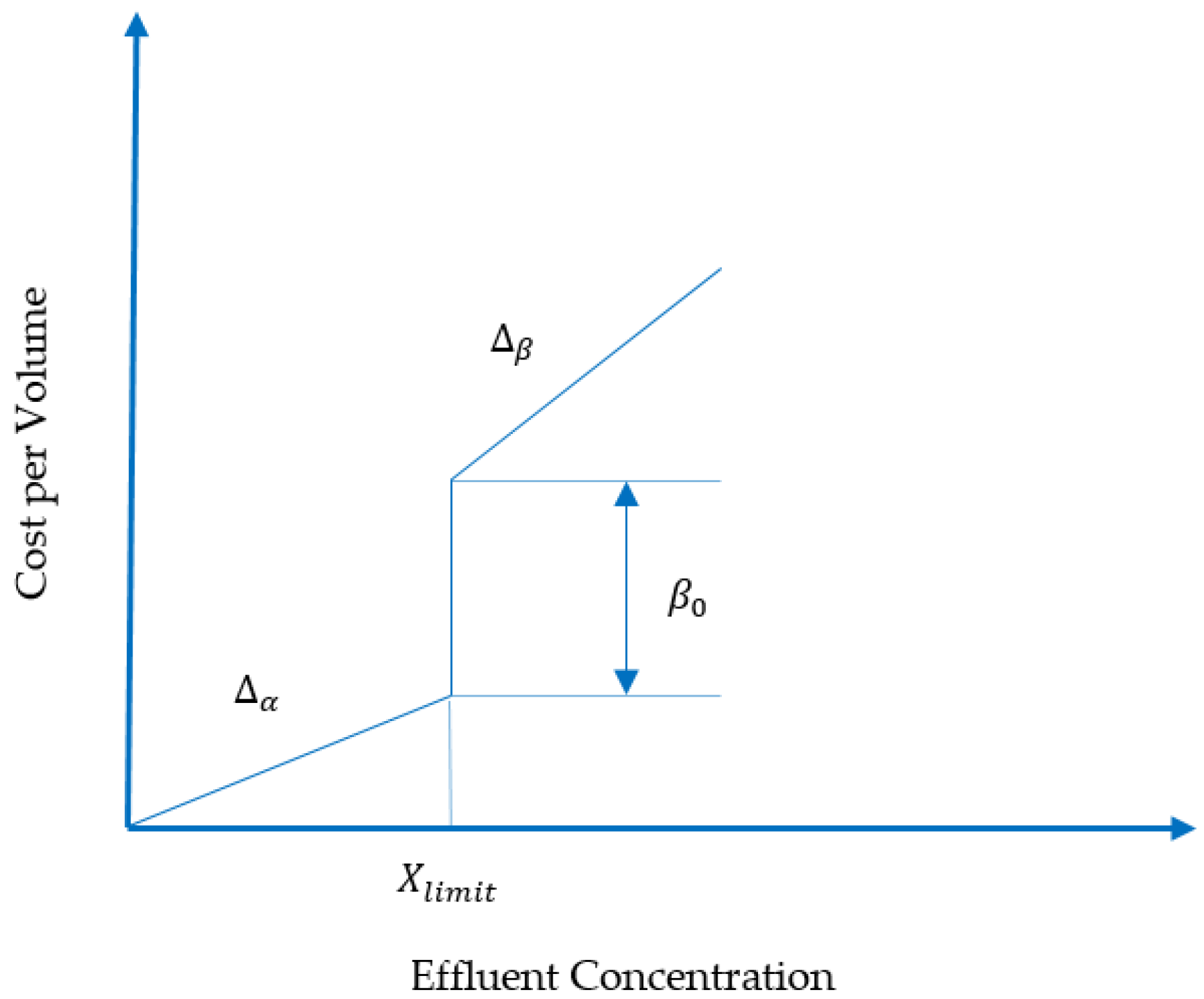
2.2. Performance Assessment

Different criteria have been defined in the benchmark to assess the performance of the plant looking for a more effective, more efficient and more sustainable solution. In our work, the proposed operating strategy to reduce the energy consumption and environmental costs is evaluated with the help of a cost index. We have called this cost index the operation cost (OC) throughout this paper. This OC provides measures of the electricity costs and the effluent quality.

Specifically, the operation cost OC is defined as follows:

$$OC\left(t\right)={\gamma }_1\left(AE\left(t\right)+ME(t\right)+PE\left(t\right))+{\gamma }_{2}SP\left(t\right)+EF\left(t\right)$$

(1)

where AE is the aeration energy (kWh), ME is the mixing energy (kWh), PE is the pumping energy (kWh), SP is the sludge production for disposal (kg) and EF stands for the effluent fines (€). Weights γ₁ and γ₂ are set in proportion to the weights in the operating cost index (OCI) defined in the benchmark (see Section 2.1).

In fact, attending to the recommendation of the BSM1, we have weighted the sludge production and the energy costs in a ratio of 5:1. Another goal of this work is to estimate the external costs of the environmental impact of electricity, so we need an estimation of the average electricity price in the EU. Finally, in the same way as Stare et al. [34], we consider 0.1 €/kWh. Hence, γ₁ = 0.1 €/kWh, and γ₂ = 0.5 €/kg.

AE is calculated by the following equation [32]:

$$AE\left(t\right)=\frac{S_0^{sat}}{1.8\times 1000}{\displaystyle \sum }_{i=3,4,5}{V}_i{K}_{L}a\left(t\right)$$

(2)

where $S_0^{sat}$ is the value of the oxygen saturation concentration, $V_i$ (i ∊ [3,5]) is the volume of the aerated reactors and $K_{L}a\left(t\right)$ the volumetric oxygen transfer coefficient in each reactor.

ME in Equation (1) is the energy used to mix the sludge in the two anoxic reactors in order to prevent from settling. It is calculated taking into account the volume in Reactors 1 and 2. ME calculation is defined in [32] and is given by:

$$ME\left(t\right)=24\times 0.005{\displaystyle \sum }_{i=1,2}{V}_i$$

(3)

PE, the pumping energy [32], is calculated as:

$$PE\left(t\right)=0.004\times Q_{in}\left(t\right)+0.008\times Q_{ext}\left(t\right)+0.05\times Q_w\left(t\right)$$

(4)

where $Q_{in}\left(t\right)$, $Q_{ext}\left(t\right)$ and $Q_w\left(t\right)$ are the internal recycle flow rate, the external recycle flow rate and the wastage flow rate, respectively.

Equation (5) shows the calculation of SP [32]:

$$SP\left(t\right)=TS{S}_w\times Q_w\left(t\right)$$

(5)

where $TS{S}_w$ is the total solid suspended in the flow wastage.

Effluent fines (EF) are calculated taking into account the discharge of pollution into receiving waters. This is calculated by weighting the different compounds of the effluent loads. In our case, in the ammonia removal process, the EF costs are caused by an excess of ammonia in the effluent [16]. Therefore, only effluent ammonia (S_NH,eff) and total nitrogen (S_TN,eff) are considered in the calculation of the EF. If X denotes either ammonia S_NH or total nitrogen S_TN, then a formal description of their effluent fines is given by (6).

$$E{F}_X\left(t\right)=Q_{eff}\left(t\right)\times \{\begin{array}{r}\mathsf{∆}{\alpha }_X{X}_{eff}\left(t\right), X_{eff}\left(t\right)\le X_{limit}\\ \mathsf{∆}{\alpha }_X{X}_{limit}+{\beta }_{0,X}+\mathsf{∆}{\beta }_X\left(X_{eff}\left(t\right)-X_{limit}\right), X_{eff}\left(t\right)>X_{limit}\end{array}$$

(6)

where X_eff (t) and Q_eff (t) are the effluent concentration and flow rate, respectively. ∆α and ∆β are the costs per kilogram of discharge below and above the effluent limit concentration X_limit. β₀ denotes the cost for exceeding the effluent limit. Figure 2 shows graphically the cost function for EF [35].

Discharge limits (X_limit) for ammonia (S_NHlimit) and total nitrogen (S_TNlimit) are set in our case to 4 and 12 mg/L, respectively. When effluent ammonia and total nitrogen are below the discharge limit, the costs of discharge are ∆α_NH = 4 €/kg and ∆α_TN = 2.7 €/kg, respectively. When the discharge limits are exceeded, the costs of discharge increase three-fold, and the costs of exceeding the discharge limits are those in

Table 1. Costs associated when discharge limits are exceeded.

∆βNH	∆βTN	β0,NH	β0,TN
12 €/kg	8.1 €/kg	2.7 €/1000 m3	1.4 €/1000 m3

[34].

Making use of the OC introduced in this section, we are showing how using a reinforcement learning approach (by designing a proper agent) allows us to maintain energy costs as low as possible, reducing the effluent fines.

3. Reinforcement Learning Approach

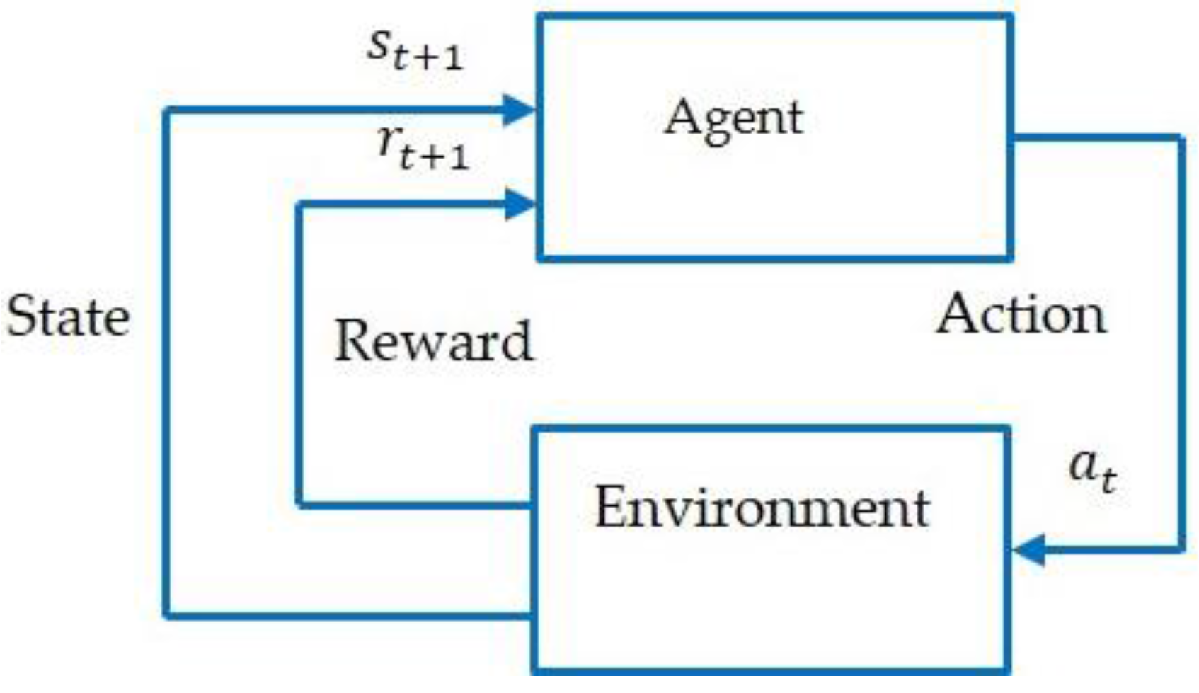
3.1. Background

The RL agents’ actions allow changing the external conditions defining an environment. To this end, there are several RL algorithms in the literature.

In order to model the interaction of the agent with the environment, a Markov decision process (MDP) is usually used. In any MDP, the state of the environment is perceived by the agent at each time step. Then, among the available different actions, the agent selects and executes one of them (see Figure 3). Consequently, the state of the environment is changed.

A more detailed description of the process is as follows. When the agent performs an action, it obtains a reward. At each step, the agent has to choose the actions in order to guarantee, over time, the sum maximization of the expected rewards. This set of actions is usually called the agent’s policy, and the agent’s goal is to find an optimal one.

The different elements that define the MDP model are: (i) a discrete space of environment states S; (ii) a discrete set of agent actions A(s); (iii) a set of transition probabilities from one state s to another state s’ once the agent has executed action a over this environment P(s’|s, a); and (iv) the expected reward to be obtained from this environment E{r|s’, a, s} when changing from state s to state s’ having executed an action a [36]. Different approaches are used to calculate the optimal policy π(s, a).

Anyway, the model of the environment is not a compulsory element in this framework. RL also supports the model-free RL algorithms [37]. In these methods, besides the optimal policy, the agent has to obtain the model of the environment.

Formally, the variables involved in the process are: t, each time step; s_t, the state of the environment observed by the agent; a_t, the action to be executed by the agent; and r_t, the reward obtained by the agent. Each action a_t generates the next state s_t+1 and reward r_t+1. The actions selected by the agent are those that increase its return. A return is defined as the long-term sum of the future reward values r_t (see Figure 3). An infinite-horizon model as follows is used when the environment is continuous:

$$R_t={\displaystyle \sum }_{t^{\prime }=t}^{\infty }{\gamma }^{\left(t^{\prime }-t\right)}{r}_t$$

(7)

where 0 < γ < 1 stands for a kind of optimization horizon (OH). In this model, not all of the rewards are taken into account in the same way. A discount factor γ (up to on) is introduced to penalize the upcoming rewards in the return R_t.

As the performance assessment of the plant in terms of energy efficiency in this research is given by (1), the main role of the agent consists of saving as much operation cost (OC) as possible. In other words, the goal of the agent is to get the energy costs as low as possible, reducing the effluent fines at the same time.

According to (7), this model-free RL agent’s goal is equivalent to lowering its return, which can be translated as the minimization of (8):

$$R_t={\displaystyle \sum }_{t^{\prime }=t}^{\infty }{\gamma }^{\left(t^{\prime }-t\right)}OC\left(t^{\prime }\right)$$

(8)

where γ stands for the time horizon of the agent’s return.

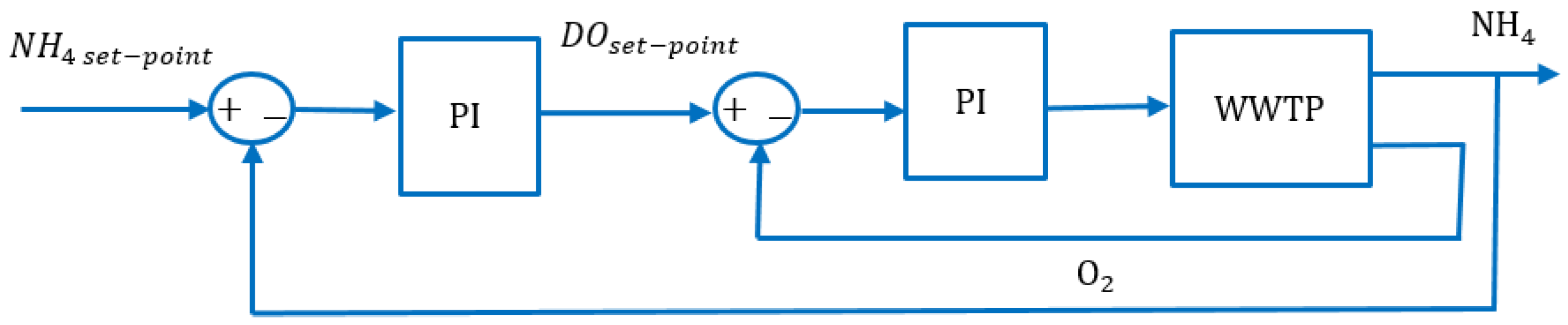
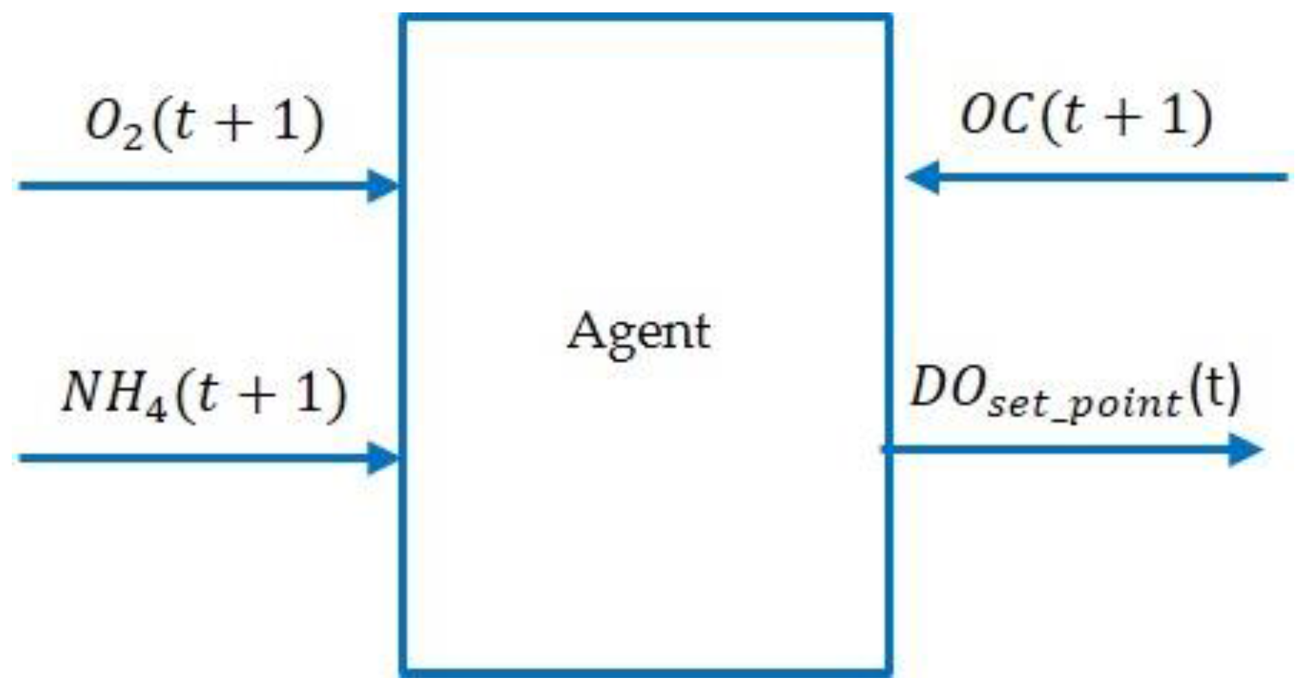
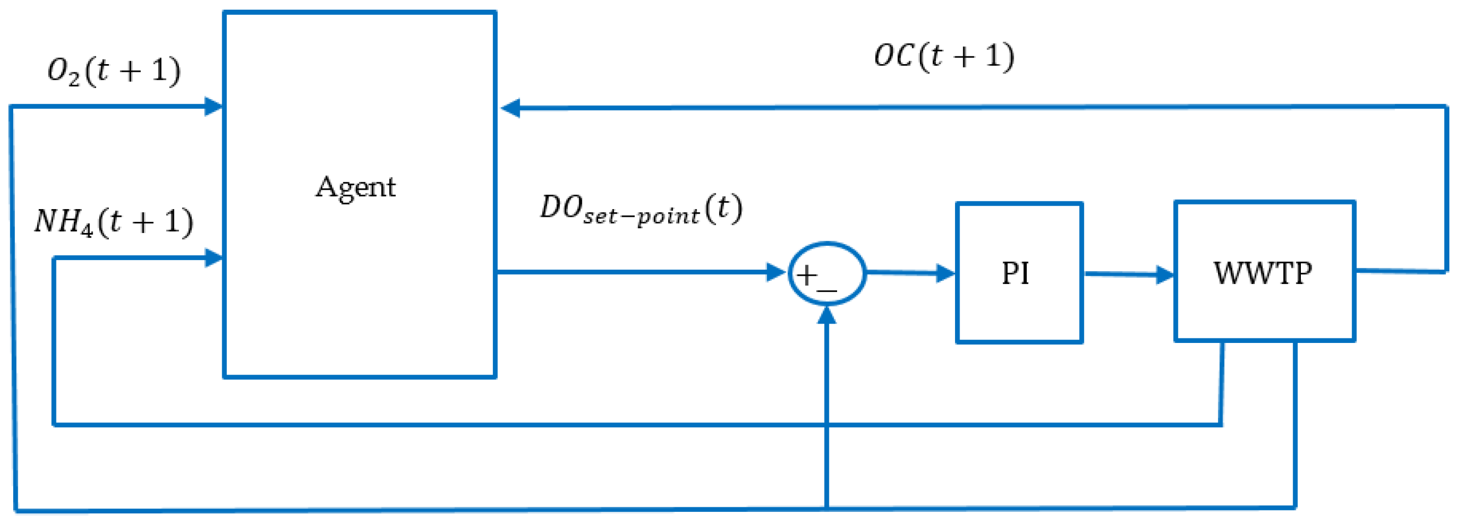
3.2. Description of the Model-Free RL Agent

A major goal in WWTPs is to keep the level of nitrogen in the effluent under a given limit (X_limit; see Section 2.2). It is possible to achieve this while improving the energy efficiency of the plant by using a model-free RL agent to tune up the DO set-point in the aerated Reactor 5. The RL agent acts as a new block in the BSM1 model.

The evolving agent [38] tunes up the dissolved oxygen (DO) set-point of a WWTP to adapt it to any plant [39]. In this paper, we will show: (i) how we can apply this method to a simulated WWTP (the BSM1); (ii) that this approach is valid in a real environment because of its fast convergence; and (iii) that it improves significantly the operation costs of the plant compared to the traditional approach based on a human operator changing the set-point for each environmental condition (365 days/24 h).

The agent is included in a simulator implemented in Modelica [40] whose model was developed in two COST Actions (624 and 682) [32]. Figure 4 shows the experimental framework. In red is highlighted the new blocks introduced in the benchmark: the weather block and the agent block. The first one defines one-year influent flow input data as a blend of 14-day chunks of the three different weather conditions.

Figure 5 shows a schematic representation of the different inputs and outputs of the agent. There are three elements we have to define to implement it: the states, the reward function and the action.

The variable s_t is the current state of the environment. Two measures are necessary to define it: NH₄ and O₂. Two sensors placed at Reactor 5 (see Section 2.1) provide these values. The agent block only has the output DO set-point, which represents the action a_t to execute. OC (t) gives the reward r_t+1 to the agent.

Algorithm 1 provides a pseudocode for the agent. In short, the instructions given to the agent are: (i) keep the ammonia low, and as best you (agent) can, try not to violate the ammonia limit; this limit, according to the BSM1 parameters, must be lower than 4 gN/m³; and (ii) keep the energy consumption as low as possible. This information is provided to the agent by means of the OC. Then, the agent acts on the plant by changing the DO set-point. In Section 4.1, we specify the different discrete set of actions over the environment used in our experiments.

Algorithm 1: RL agent method

Configuration  γ: Time horizon  max_actions = 2//maximum number of actions  DO_max: Set-point max  DO_min: Set-point min  DO_step: Set-point step (DO_step = (DO_max-DO_min)/(max_actions+1)) Inputs  s(t) = [NH4(t),O2(t)]: State of the environment  r(t) = −OC(t): reward Output  DO: Real Internal  Q(s,a): initialize arbitrarily  a: action (0..max_actions) Algorithm  Initialize Q(s,a);  while (true) {//execute every 15 minutes   s(t) = [NH4,O2];   r(t) = −OC(t);   a = next_action(Q,s);   update_Q(s,a,r);   DO = DO_min + a*DO_step;   execute(DO);  }

The procedures performed by the agent are implemented in a dedicated library that is coded in C. From Modelica, the agent is called to get the values of the state variables (measures of NH₄ and O₂), to obtain the value of the reward (OC(t)) and to calculate the action (value for DO set-point).

Finally, it is important to note that, in the WWTP, the blower of Reactor 5 is controlled, as usual, by means of a PI controller (see Figure 6). The feedback loop of this PI is closed by an error signal, which consists of the difference between the dissolved oxygen (DO) level (of Reactor 5) and the DO set-point. This set-point is autonomously changed using the RL agent.

4. Simulation Results

4.1. Experiment Settings

The model-free RL agent has to learn the model of its environment and how to best behave on it by systematic trial and error. As the provided influent profiles in the BSM1 correspond to dry, rainy and stormy weather conditions, the discrete set of actions over the environment are set as three optimal DO set-points calculated for each of these possible environmental conditions: 1.2 mg/L, 1.5 mg/L and 1.85 mg/L for dry, stormy and rainy weather, respectively. In this way, the agent’s policy must choose among these actions. Additionally, this choice is done every 15 min, as the dynamic flow rate profiles are sampled in the BSM1 with an interval of 15 min. Moreover, it must be noticed that 15 min is enough time to let the oxygen get the set-point and also to compute the agent’s decision. In addition, more time would leave less freedom to the agent.

The optimization horizon considered in the agent’s return is one month, which means that the OC is averaged over a monthly observation period.

The weather block (see Section 3.2 and Figure 4) allows us to define different weather profiles. In this experiment, the weather profile over one year is shown in Figure 7. The three possible environmental conditions, dry, rainy and stormy weather, are taken into account in our experiments. The weather varies randomly in the following way: it rains 20% of the time, and it storms 10% of the time. Thus, the remaining 70% of the time, the weather is dry.

The main goal of the proposed experiments is to compare the agent’s behavior with the human’s. In the following, we are simulating a perfect human behavior, the so-called ideal operator, as a human who can change the DO set-point to the optimal one whenever needed. In this way, the ideal operator: (i) has complete knowledge of the weather (at any time); (ii) is able to set immediately the DO set-point when required (when a weather change occurs); (iii) can perform this action at any time (365 days/year, 24 h/day).

Something important to notice is that the RL agent does not have complete knowledge of the weather (as the ideal operator does). It only accesses the oxygen and the N-ammonia inputs (see Figure 5). In this sense, our RL agent can be considered as a real agent. In what follows, we compare a real agent with an ideal operator.

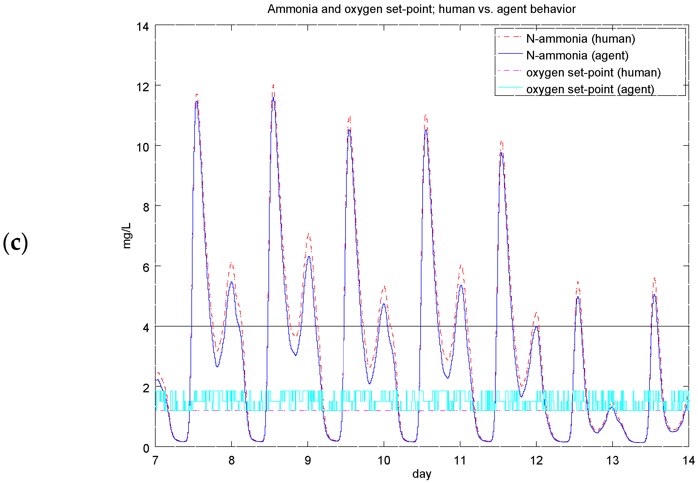
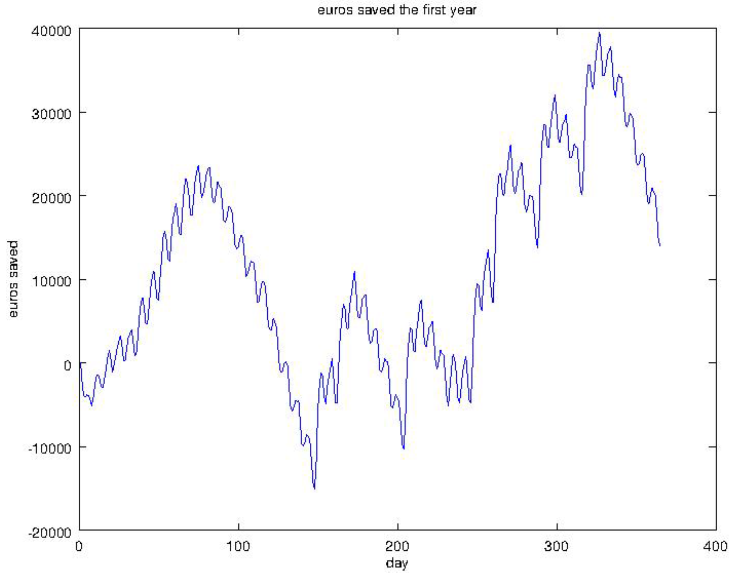
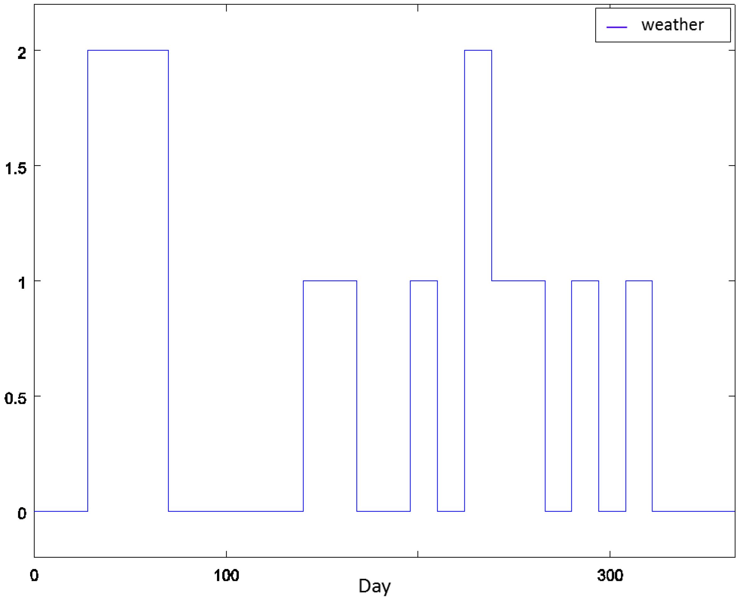
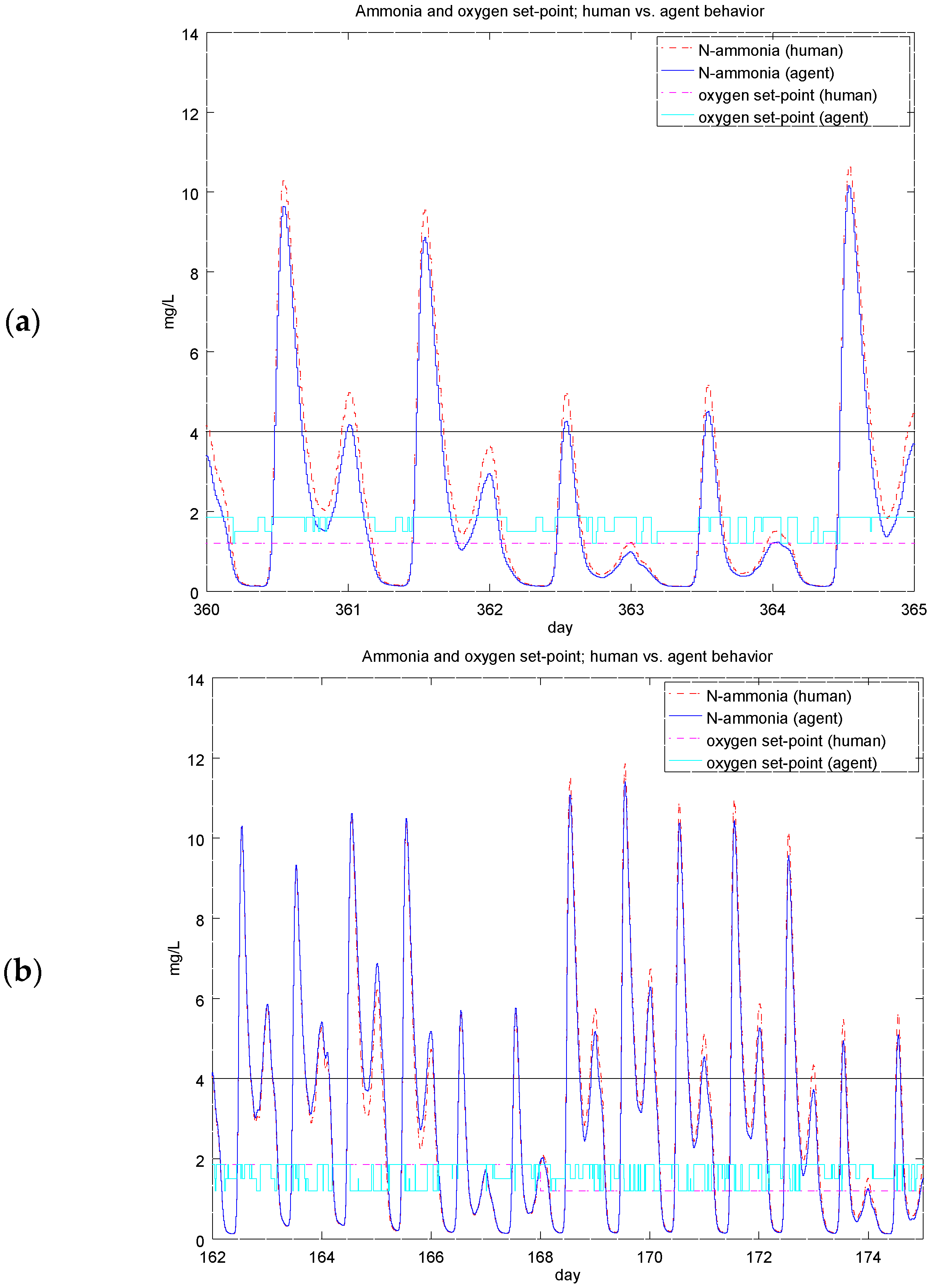
4.2. Experiment 1: Analysis of the RL Agent's Behavior

This experiment focuses on comparing the agent’s behavior against the human’s behavior (ideal operator) as the test base (see Figure 8). We also show how quick the RL agent learns and how this behavior tends to be less noisy as the learning evolves.

Figure 8a shows the behavior at the last days of the year. In this case, the agent has been learning during one year, and the weather is dry (see Figure 7). The human operator keeps a constant oxygen set-point to 1.2 mg/L (the optimal set-point in a forever dry-weather condition). However, as Figure 8a shows, our RL agent has learned that the optimal behavior is to keep the oxygen set-point over 1.2 mg/L. The agent changes the set-point every 15 min, not only when the weather changes, lowering the operation cost. Notice that, in order to keep the fines as low as possible (under 4 mg/L), the RL agent keeps the DO set-point time higher than the operator does. In fact, the RL agent tries to keep the N-ammonia under 4 mg/L to reduce the cost of fines. At the same time, it lows the DO set-point (then the energy) when the N-ammonia in the effluent is far away from the limit (i.e., see Day 363, Figure 8a).

Figure 8b corresponds to a more dynamic weather behavior. In this case, the weather condition changes from rainy weather to dry weather. This change happens in Day 168 (see Figure 7). This dynamic behavior in the weather profile leads the agent to have a more dynamic behavior, as well. At the beginning of this simulation (days from 162 to 166), the weather is rainy. In these days, the agent detects that keeping the oxygen as high as the human operator does not improve the costs due to the fines. Thus, the agent decreases the DO set-point in order to reduce the energy costs. This agent’s behavior has to do with the small reduction of the fine costs in a rainy weather condition, where the N-ammonia concentration is higher than 4 mg/L for a longer period of time. The opposite occurs when the weather condition changes to dry from Day 168.

Figure 8c shows the agent’s behavior in the first days of the year. The agent has been learning for six days (it starts from scratch at Day 1). It can be observed that even as early as the 12th day, it has learned to reduce the N-ammonia concentration below 4 mg/L. It can be seen that the agent increases the DO set-point in the critical moments to reduce the N-ammonia concentration.

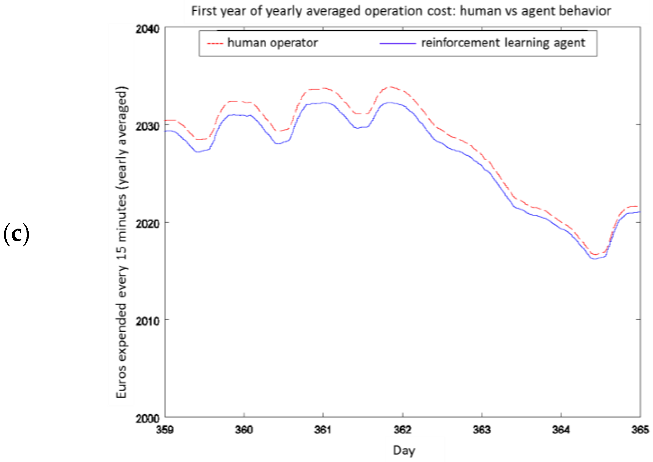
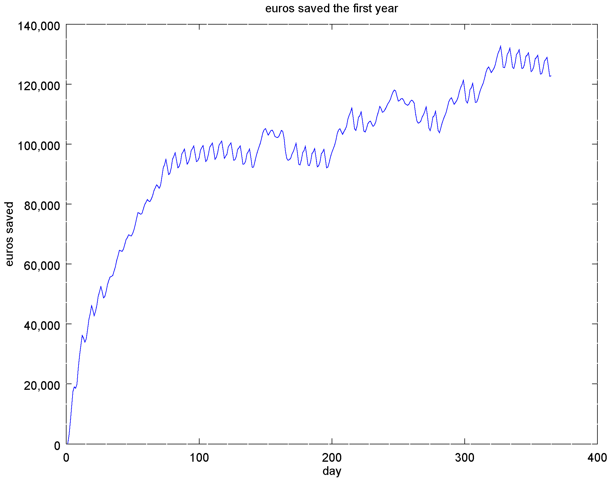
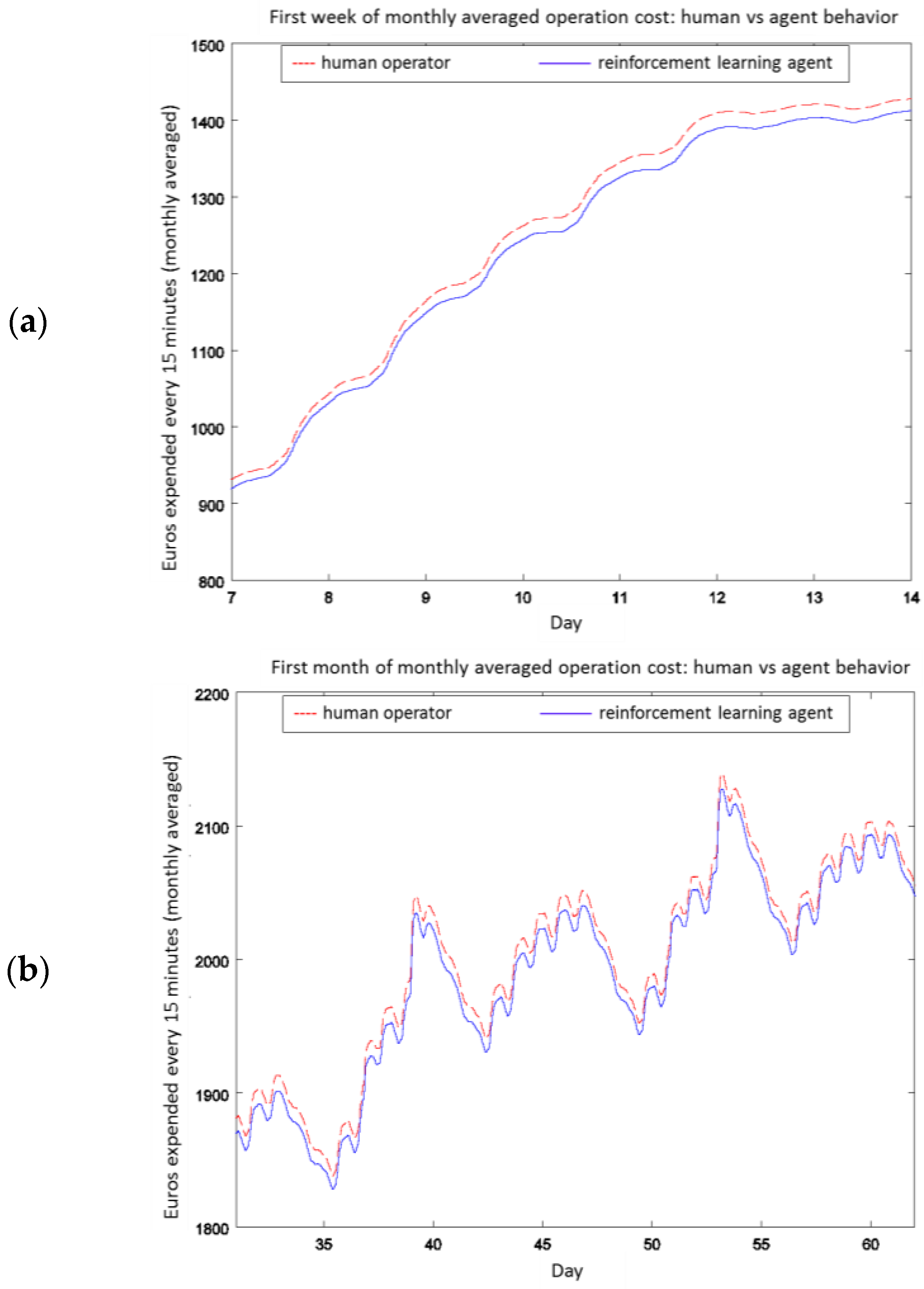
4.3. Experiment 2: Analysis of the Energy Efficiency and Environmental Costs

In this experiment, we are showing how the RL agent gets an improvement in the operation cost (which implies energy efficiency). We are comparing the operation costs of the agent’s behavior to the human’s one. Figure 9 shows the averaged costs during the first week, first month and a whole year, respectively.

In Figure 9a,b, a monthly averaged cost has been used. It can be observed that the agent learns fast enough to be useful from the very first time. In Figure 9c, a comparison of the yearly averaged costs at the end of the year is shown.

Figure 10 shows an important result: the global saved costs during the whole first year day after day. It has been calculated as the cumulative difference in euros between the human operator and the agent. This difference is calculated every 15 min and added up without any average.

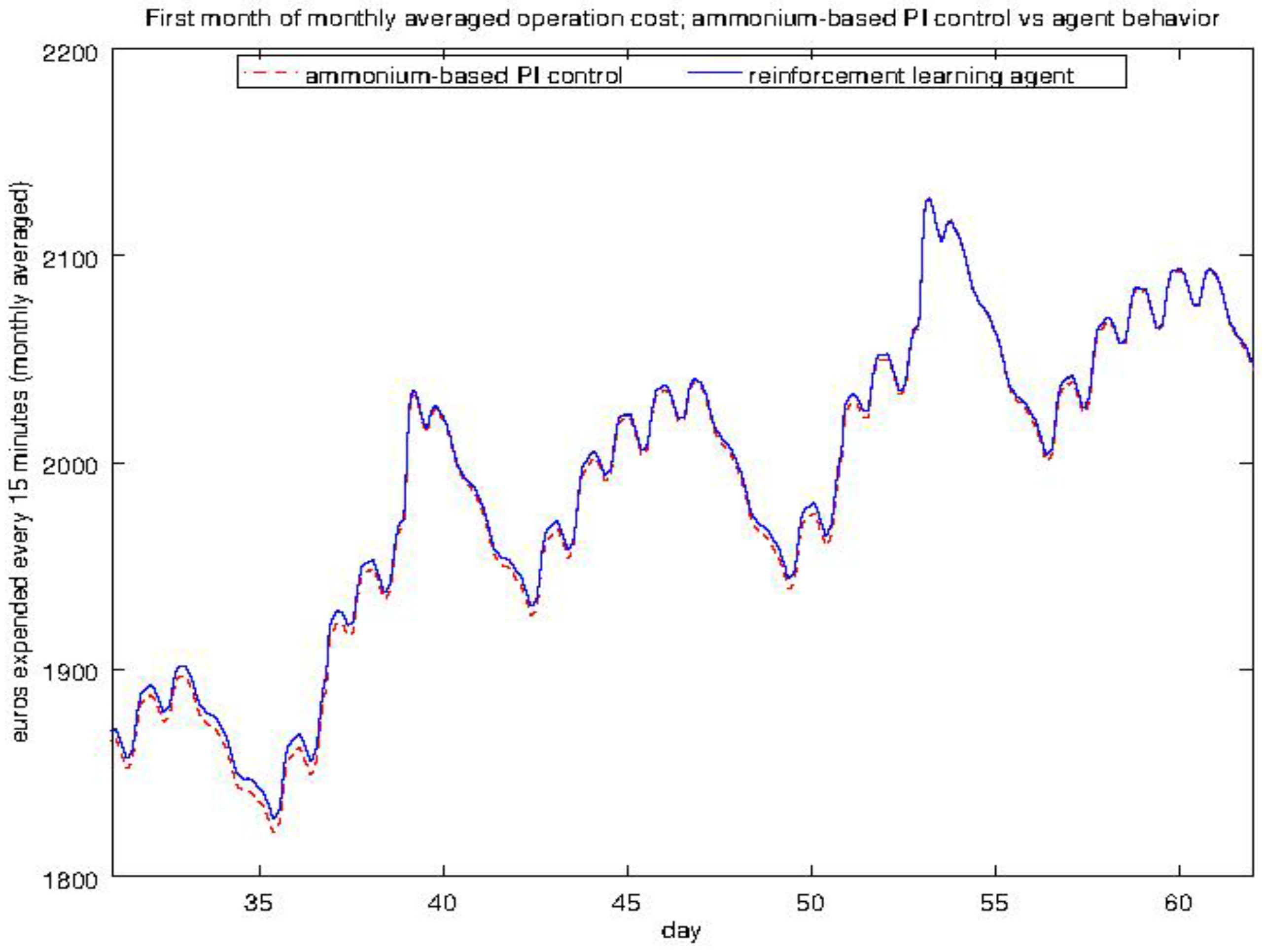
4.4. Experiment 3: Ammonium-Based PI Control versus the RL Agent Approach

Apart from having a human plant operator in charge of setting the DO set-point, another way to control the DO set-point is by a PI cascade control structure, as the shown in Figure 11 [41].

The measure of the ammonium concentrations in the outlet of the activated sludge process is used to obtain the value of the DO set-point. It can also be done with an in situ sensor.

In order to get a more complete evaluation of the agent, we have compared the agent’s behavior against an ammonium-based PI control as the test base. Figure 12 shows the global saved costs during the whole first year, day after day, when using the ammonium-based PI control. It has been calculated as the cumulative difference in euros between the ammonium-based PI structure and the RL agent. This difference is calculated every 15 min and added up without any average. Figure 10 and Figure 12 show that the RL agent saves OC during the first year either using the human operator or the ammonium-based PI control. However, a more detailed study is left as future work (see Section 5). Furthermore, Figure 13 and Figure 14 show a comparison between the RL agents’ behavior and the ammonia-based PI control.

5. Conclusions

Wastewater treatment plants are key infrastructures for ensuring the proper protection of our environment. However, these plants are also major energy consumers, and they must work efficiently to avoid environmental problems. Although efforts have been made to solve these problems, many WWTPs are still operated in a less than optimal manner with respect to energy and environmental efficiency.

In this paper, a reinforcement learning approach is included in the BSM1 to save costs in the N-ammonia removal process. The RL agent allows a quick and autonomous adaptation of the plant to changes in the environmental conditions with a minimal intervention of the plant operator. This is done by tuning up the DO set-point autonomously, without needing an external expert.

In conclusion, the main implication of this approach is that in each different place (country or city), the adaptation of the agent is achieved in an autonomous way. Therefore, it can be considered as a solution for addressing energy efficiency in different scenarios. For instance, a major challenge in small wastewater treatment systems is how to finance the high tuning costs of the process. The same happens in plants located in places with unstable environmental conditions. This approach not only helps the plant operator, but also helps to reduce costs because of its more efficient behavior. This fact is shown in the reduction obtained in the operation cost, which quantifies both energy and environmental costs.

As future work, we plan to compare the RL agent with more complex PI-based techniques [41] as we did preliminarily in this paper. Furthermore, we intend to implement and test the RL agent in a real case scenario to analyze the energy savings by comparing the idealized human and plant with an existing plant and human operation case. Due to the non-linearity of the process a detailed analysis of the uncertainties in the system will be required when addressing the tests of the proposed approach in a real plant [42,43]. Moreover, sensor validation procedures will be essential to ensure the good performance of the proposed framework in a real situation. It is remarkable that the proposed RL agent explicitly takes into account the input disturbance. In this way, the agent has the capacity of developing a new behavior by itself in order to adapt to each new scenario.

References

- Al-Dosary, S.; Galal, M.M.; Abdel-Halim, H. Environmental Impact Assessment of Wastewater Treatment Plants. Int. J. Curr. Microbiol. App. Sci. 2015, 4, 953–964. [Google Scholar]
- Awad, E.S.; Al Obaidy, A.H.; Al Mendilawi, H.R. Environmental Assessment of Wastewater Treatment Plants (WWIPs) for Old Rustamiya Project. Int. J. Sci. Eng. Technol. Res. 2014, 3, 3455–3459. [Google Scholar]
- Jeon, E.C.; Son, H.K.; Sa, J.H. Emission Characteristics and Factors of Selected Odorous Compounds at a Wastewater Treatment Plant. Sensors 2009, 9, 311–326. [Google Scholar] [CrossRef] [PubMed]
- Eslamian, S. Urban Water Reuse Handbook; Taylor & Francis Group: New York, NY, USA, 2016. [Google Scholar]
- Brandt, M.J.; Middleton, R.A.; Wang, S. Energy Efficiency in the Water Industry: A Compendium of Best Practices and Case Studies UKWIR Report 10/CL/11/3; Water Research Foundation: London, UK, 2010. [Google Scholar]
- Energy Best Practices Guide: Water & WateWater Industry. Available online: http://dnr.wi.gov/aid/documents/eif/focusonenergy_waterandwastewater_guidebook.pdf (accessed on 29 June 2016).
- Crawford, G.; Sandino, J. Energy Efficiency in Wastewater Treatment in North America: A Compendium of Best Practices and Case Studies of Novel Approaches; Water Research Foundation: London, UK, 2010. [Google Scholar]
- Eskaf, S. Four Trends in Government Spending on Water and Wastewater Utilities since 1956. Available online: http://efc.web.unc.edu/2015/09/09/four-trends-government-spending-water/ (accessed on 30 June 2016).
- Cristea, S.; de Prada, C.; Sarabia, D.; Gutiérrez, G. Aeration control of a wastewater treatment plant using hybrid NMPC. Comput. Chem. Eng. 2011, 35, 638–650. [Google Scholar] [CrossRef]
- Chachuat, B.; Roche, N.; Latifi, M.A. Dynamic optimisation of small size wastewater treatment plants including nitrification and denitrification processes. Comput. Chem. Eng. 2001, 25, 585–593. [Google Scholar] [CrossRef]
- Revollar, S.; Vega, P.; Vilanova, R. Economic optimization of Wastewater Treatment Plants using Non Linear Model Predictive Control. In Proceedings of the 2015 19th International Conference on System Theory, Control and Computing (ICSTCC), Judetul Brasov, Romania, 14–16 October 2015; pp. 583–588.
- Metcalf-Eddy Inc.; Tchobanoglous, G.; Burton, F.L.; Stensel, H.L. Wastewater Engineering: Treatment and Reuse, 4th ed.; McGraw-Hill Higher Education: New York, NY, USA, 2002. [Google Scholar]
- Yang, T.; Qiu, W.; Ma, Y.; Chadli, M.; Zhang, L. Fuzzy model-based predictive control of dissolved oxygen in activated sludge processes. Neurocomputing 2014, 136, 88–95. [Google Scholar] [CrossRef]
- Holenda, B.; Domokos, E.; Rédey, Á.; Fazakas, J. Dissolved oxygen control of the activated sludge wastewater treatment process using model predictive control. Comput. Chem. Eng. 2008, 32, 1270–1278. [Google Scholar] [CrossRef]
- Vilanova, R.; Katebi, R.; Wahab, N. N-Removal on Wastewater Treatment Plants: A Process Control Approach. J. Water Resour. Prot. 2011, 3, 1–11. [Google Scholar] [CrossRef]
- Samuelsson, P.; Halvarsson, B.; Carlsson, B. Cost-efficient operation of a denitrifying activated sludge process. Water Res. 2007, 41, 2325–2332. [Google Scholar] [CrossRef] [PubMed]
- Rojas, J.; Zhelev, T. Energy efficiency optimization of wastewater treatment: Study of ATAD. Comput. Chem. Eng. 2012, 38, 52–63. [Google Scholar] [CrossRef]
- Henze, M.; Gujer, W.; Mino, T.; van Loosdrecht, M.C.M. Activated Sludge Models ASM1, ASM2, ASM2d and ASM3 Technical Report; International Water Association (IWA): London, UK, 2000. [Google Scholar]
- Olsson, G.; Nielsen, M.; Yuan, Z.; Lynggaard-Jensen, A.; Steyer, J. Instrumentation, Control and Automation in Wastewater Systems; International Water Association (IWA): London, UK, 2005. [Google Scholar]
- Bennett, A. Energy efficiency: Wastewater treatment and energy production. Filtr. Sep. 2007, 44, 16–19. [Google Scholar] [CrossRef]
- Meneses, M.; Concepción, H.; Vilanova, R. Joint Environmental and Economical Analysis of Wastewater Treatment Plants Control Strategies: A Benchmark Scenario Analysis. Sustainability 2016, 8, 360. [Google Scholar] [CrossRef]
- Caraman, S.; Sbarciog, M.; Barbu, M. Predictive Control of a Wastewater Treatment Process. IFAC Proc. Vol. 2006, 39, 155–160. [Google Scholar] [CrossRef]
- O’Brien, M.; Mack, J.; Lennox, B.; Lovett, D.; Wall, A. Model predictive control of an activated sludge process: A case study. Control Eng. Pract. 2011, 19, 54–61. [Google Scholar] [CrossRef]
- Lindberg, C.; Carlsson, B. Nonlinear and set-point control of the dissolved oxygen concentration in an activated sludge process. Water Sci. Technol. 1996, 34, 135–142. [Google Scholar] [CrossRef]
- Hong, G.; Kwanho, J.; Jiyeon, L.; Jeongwon, J.; Young, M.K.; Jong, P.P.; Joon, H.K.; Kyung, H.C. Prediction of effluent concentration in a wastewater treatment plant using machine learning models. J. Environ. Sci. 2015, 101, 32–90. [Google Scholar]
- Celik, U.; Yuntay, N.; Sertkaya, C. Wastewater effluent prediction based on decisión tree. J. Selcuk Univ. Nat. Appl. Sci. 2013, 138–148. [Google Scholar]
- Huang, M.; Ma, Y.; Wan, J.; Chen, X. A sensor-software based on a genetic algorithm-based neural fuzzy system for modeling and simulating a wastewater treatment process. Appl. Soft Comput. 2015, 27, 1–10. [Google Scholar] [CrossRef]
- Bagheri, M.; Mirbagheri, S.A.; Bagheri, Z.; Kamarkhani, A.M. Modeling and optimization of activated sludge bulking for a real wastewater treatment plant using hybrid artificial neural networks-genetic algorithm approach. Process Saf. Environ. Prot. 2015, 95, 12–25. [Google Scholar] [CrossRef]
- Han, H.; Qiao, J.; Chen, Q. Model predictive control of dissolved oxygen concentration based on a self-organizing RBF neural network. Control Eng. Pract. 2012, 20, 465–476. [Google Scholar] [CrossRef]
- Syafiie, S.; Tadeo, F.; Martinez, E.; Alvarez, T. Model-free control based on reinforcement learning for a wastewater treatment problem. Appl. Soft Comput. 2011, 11, 73–82. [Google Scholar] [CrossRef]
- Alex, J.; Benedetti, L.; Copp, J.B.; Gernaey, K.V.; Jeppsson, U.; Nopens, I.; Pons, M.N.; Rieger, L.; Rosen, C.; Steyer, J.P.; et al. Benchmark Simulation Model No. 1 (BSM1). Available online: http//www.iea.lth.se/publications/Reports/LTH-IEA-7229.pdf (accessed on 26 May 2016).
- Copp, J. The COST Simulation Benchmark: Description and Simulator Manual; Office for Official Publications of the European Community: Luxembourg, Luxembourg, 2002. [Google Scholar]
- Takács, I.; Patry, G.G.; Nolasco, D. A dynamic model of the clarification thickening process. Water Res. 1991, 25, 1263–1271. [Google Scholar] [CrossRef]
- Stare, A.; Vrecko, D.; Hvala, N.; Strmcnik, S. Comparison of control strategies for nitrogen removal in activated sludge process in terms of operating costs: A simulation study. Water Res. 2007, 41, 2004–2014. [Google Scholar] [CrossRef] [PubMed]
- Vanrolleghem, P.A.; Jeppsson, U.; Carstensen, J.; Carlsson, B.; Olsson, G. Integration of wastewater treatment plant design and operation—A systematic approach using cost functions. Water Sci. Technol. 1996, 34, 159–171. [Google Scholar] [CrossRef]
- Hernández-del-Olmo, F.; Gaudioso, E. Reinforcement Learning Techniques for the Control of WasteWater Treatment Plants. Lecture Notes Comput. Sci. 2011, 6687, 215–222. [Google Scholar]
- Busoniu, L.; Babuska, R.; De Schutter, B.; Ernst, D. Reinforcement Learning and Dynamic Programming Using Function Approximators; CRC Press: Boca Raton, FL, USA, 2010. [Google Scholar]
- Hernández-del-Olmo, F.; Llanes, F.H.; Gaudioso, E. An emergent approach for the control of wastewater treatment plants by means of reinforcement learning techniques. Expert Syst. Appl. 2012, 39, 2355–2360. [Google Scholar] [CrossRef]
- Hernández-del-Olmo, F.; Gaudioso, E.; Nevado, A. Autonomous adaptive and active tuning up of the dissolved oxygen setpoint in a wastewater treatment plant using reinforcement learning. IEEE Trans. Syst. Man Cybern. Part C Appl. Rev. 2012, 42, 768–774. [Google Scholar] [CrossRef]
- Fritzson, P. Principles of Object-Oriented Modeling and Simulation with Modelica 3.3: A Cyber-Physical Approach; Wiley-IEEE Press: Pistacaway, NJ, USA, 2014. [Google Scholar]
- Åmand, L.; Olsson, G.; Carlsson, B. Aeration control—A review. Water Sci. Technol. 2013, 67, 2374–2398. [Google Scholar] [CrossRef] [PubMed]
- Belia, E.; Neumann, M.B.; Benedetti, L.; Johnson, B.; Murthy, S.; Weijers, S.; Vanrolleghem, P.A. Uncertainty in Wastewater Treatment Design and Operation: Addressing Current Practices and Future Directions; Scientific and Technical Report Series; International Water Association (IWA): London, UK, 2016. [Google Scholar]
- Sin, G.; Gernaey, K.V.; Neumann, M.V.; Van Loosdrecht, M.C.; Gujer, W. A Global sensitivity analysis in wastewater treatment plant model applications: Priorizing sources of uncertainty. Water Res. 2011, 45, 639–651. [Google Scholar] [CrossRef] [PubMed]