Maintenance Maneuver Automation for an Adapted Cylindrical Shape TEC

Abstract

Several manufacturers have developed devices with which to harness tidal/current power in areas where the depth does not exceed 40 m. These are the so-called first generation Tidal Energy Converters (TEC), and they are usually fixed to the seabed by gravity. When carrying out maintenance tasks on these devices it is, therefore, necessary to remove the nacelles from their bases and raise them to the surface of the sea. They must subsequently be placed back on their bases. These tasks require special high performance ships, signifying high maintenance costs. The automation of emersion and immersion maneuvers will undoubtedly lead to lower costs, given that ships with less demanding requirements will be required for the aforementioned maintenance tasks. This research presents a simple two degrees of freedom dynamic model that can be used to control a first generation TEC that has been conceived of to harness energy from marine currents. The control of the system is carried out by means of a water ballast system located inside the nacelle of the main power unit and is used as an actuator to produce buoying vertical forces. A nonlinear control law based on a decoupling term for the closed loop depth and/or orientation control is also proposed in order to ensure adequate behavior when the TEC performs emersion and immersion maneuvers with only hydrostatic buoyancy forces. The control scheme is composed of an inner loop consisting of a linear and decoupled input/output relationship and the vector of friction and compressibility terms and an outer loop that operates with the tracking error vector in order to ensure the asymptotically exponential stability of the TEC posture. Finally, the effectiveness of the dynamic model and the controller approach is demonstrated by means of numerical simulations when the TEC is carrying out an emersion maneuver for the development of general maintenance tasks and an emersion maneuver for blade-cleaning maintenance tasks.

1. Introduction

Tidal energy is a renewable source that may both help attain the EU climate change targets and provide additional value in a future energy market with regard to other renewable energy sources thanks to its high predictability [1,2]. Some of its principal opportunities and benefits include energy independence, job creation, decarbonization or serving as a complement to other renewable sources within the global energy mix. Several manufacturers are developing devices that can be used to harness tidal/current power in areas in which the depth does not exceed 40 m [3,4,5,6,7]. 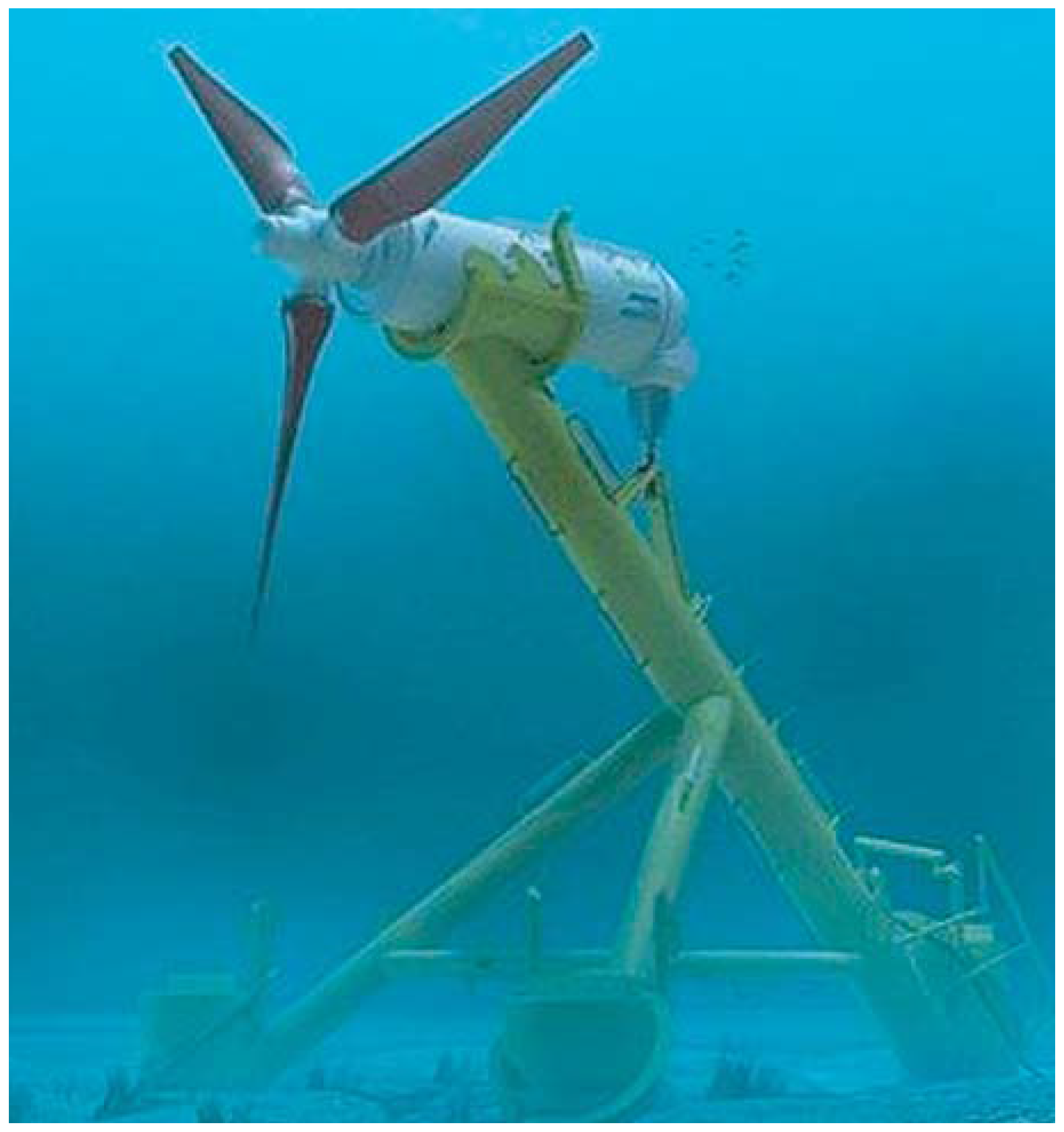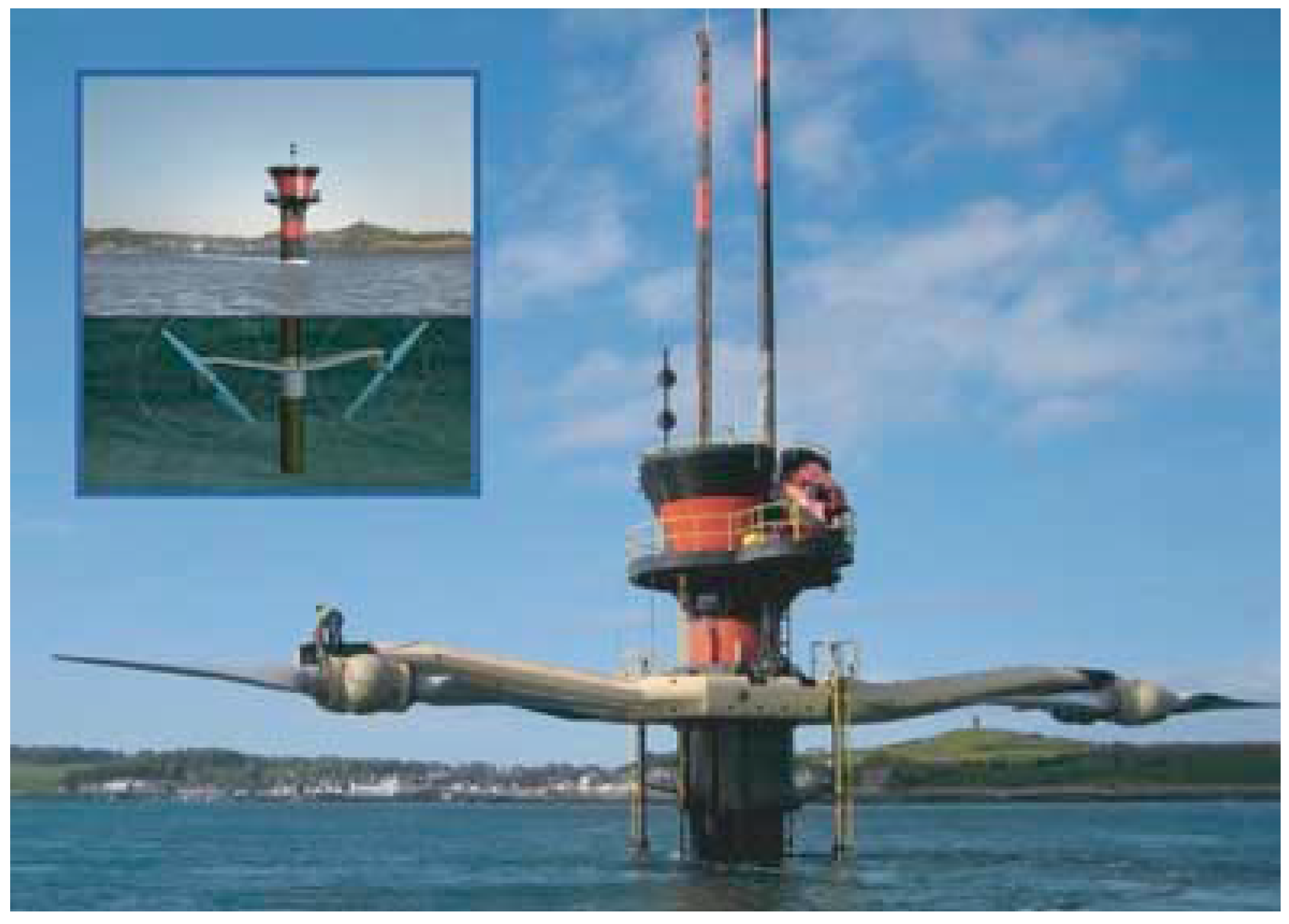Figure 1 depicts an example of Tidal Energy Converters (TEC) based on an open rotor configuration for marine current harnessing. These devices are usually supported on a base that is fixed to the seabed with different anchoring systems, and these are the so-called first generation TEC. 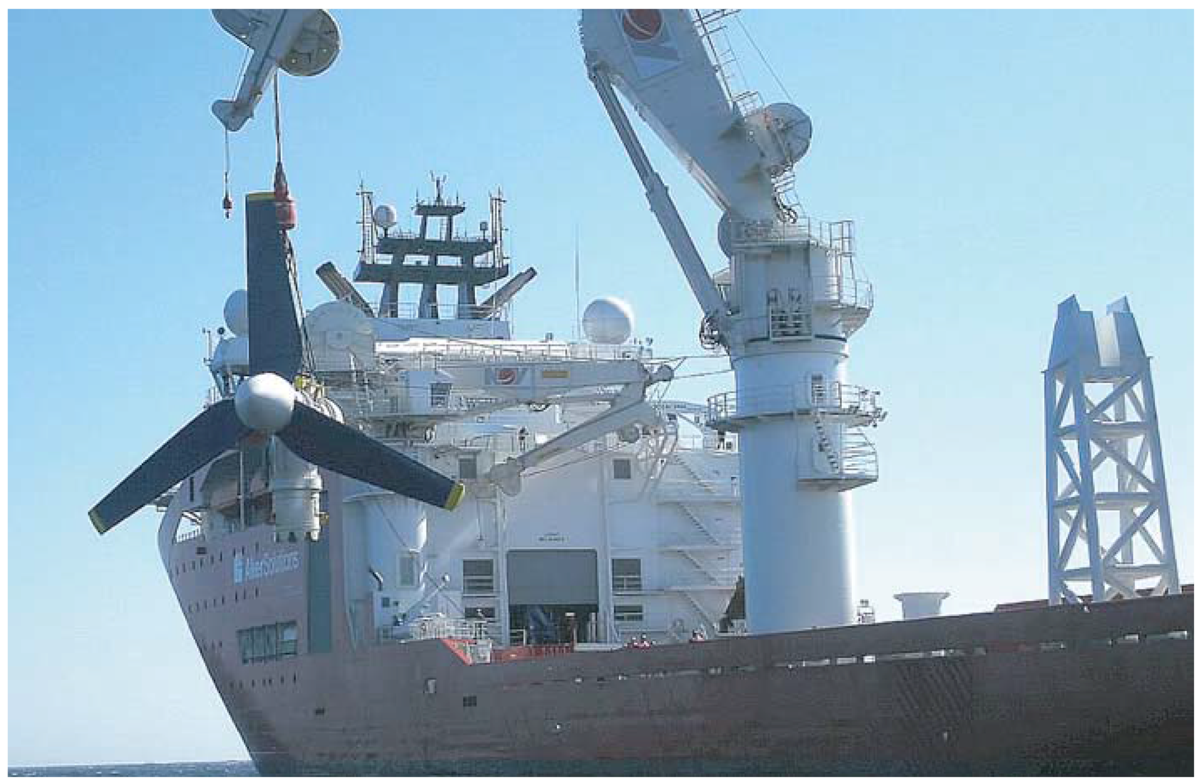Figure 2, meanwhile, shows a well-known device that uses a fixed structure that is anchored to the seabed and provided with a servo-actuated crabbing-based system in order to move its two main generation units from the underwater depth of operation to the sea surface and vice versa [8]. In the case of fully-submerged devices, maintenance tasks require the main power units (which include the Power-Take-Off (PTO)) to be disconnected from the base to allow them to be extracted from the water [9,10]. These procedures should be designed to provide high reliability and to be performed with an appropriate “weather window”, thus resulting in the reduction of associated costs [11]. Special high performance ships equipped with dynamic positioning, large cranes, etc., are required for these tasks, which means high maintenance costs. Figure 3 shows an example of the kind of setup needed to handle the main power unit of a first-generation TEC.

It is necessary to promote awareness of ocean technologies like wave energy [13], tidal energy [14], off-shore wind energy [15] salinity and thermal gradients energy [16] and increase their actual potential, and this depends on cost-effectiveness, reliability, survivability and accessibility. Regarding the tidal energy, this can be achieved by reducing installation, operation and maintenance costs by performing the emersion and immersion maneuvers in an automatized manner, which will help the acceleration and sustainability of these energy systems [4,17,18]. In [19] the automatic maneuvering emersion and immersion of one of these devices is studied. Nowadays, there exist different devices with the following main alternatives for performing maintenance tasks:

• Use of a servo-actuated crabbing-based system to move the main generation unit from the support structure [20,21].
• Use of elevation and placement by means of floating cranes [7,10,22].
• Use of a ballast management system to generate vertical forces, thus enabling the devices’ emersion and immersion movements to be controlled [6,9,23,24].

The automation of emersion and immersion maneuvers will have a direct influence in the following respects: (a) the development of improved installation procedures that will reduce the number and duration of installation operations; (b) a reduction in the cost of energy; (c) an increase in the profitability of the project; (d) less human intervention; (e) the maximization of the weather window; and (f) the possibility of using less expensive general purpose ships as tugboats rather than high cost special vessels for maintenance purposes.

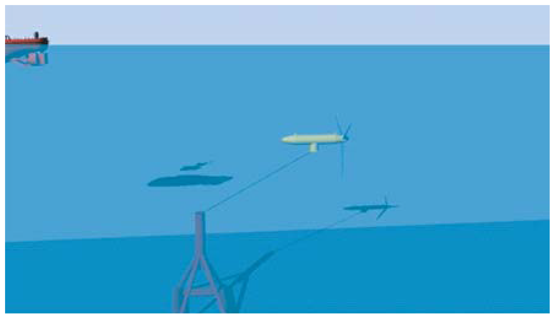
One of the first steps that should be taken to accomplish these maneuvers automatically is that of implementing a closed loop depth and/or orientation control in order to: (i) extract the main power generation unit from its normal depth of operation (on the base placed on the seabed) to the sea surface and then; (ii) return it from the sea surface to the base. These automatic maneuvers can be performed by controlling the inner ballast water inside the device and with the help of small guide wires, as is illustrated in Figure 4 [25]. As a previous step to performing automatic emersion/immersion maneuvers, it is necessary to obtain dynamic models of submerged bodies, with a good correspondence with real responses, which requires minimum computational effort, from which control schemes can be developed [26,27,28,29].

This work presents a very simple dynamic modeling and a nonlinear control for a cylindrically-shaped nacelle adapted from a first generation TEC. The dynamic model for an approximately cylindrical body is composed of only two lumped masses handled solely by hydrostatic forces, which are conceived of as volume-increasing devices. It is, meanwhile, necessary to design the nonlinear control law on the basis of an uncoupling term and nonlinear term compensation for the closed loop depth and/or orientation control in order to ensure adequate behavior when the TEC performs emersion and immersion maneuvers with only passive buoyancy forces.

The paper is structured as follows: Section 2 describes the dynamic model proposed for the first generation TEC when performing two degrees-of-freedom motions. The derivation of the nonlinear control law is presented in Section 3. Section 4 shows the numerical simulations obtained to illustrate the behavior of the proposed dynamic model and the proposed control algorithm when the TEC is carrying out an emersion maneuver for high maintenance tasks and an emersion maneuver for the development of blade-cleaning maintenance tasks. Finally, Section 5 shows our conclusions and proposals for future works.

2. Dynamic Model of a Cylindrically-Shaped Tidal Energy Converter

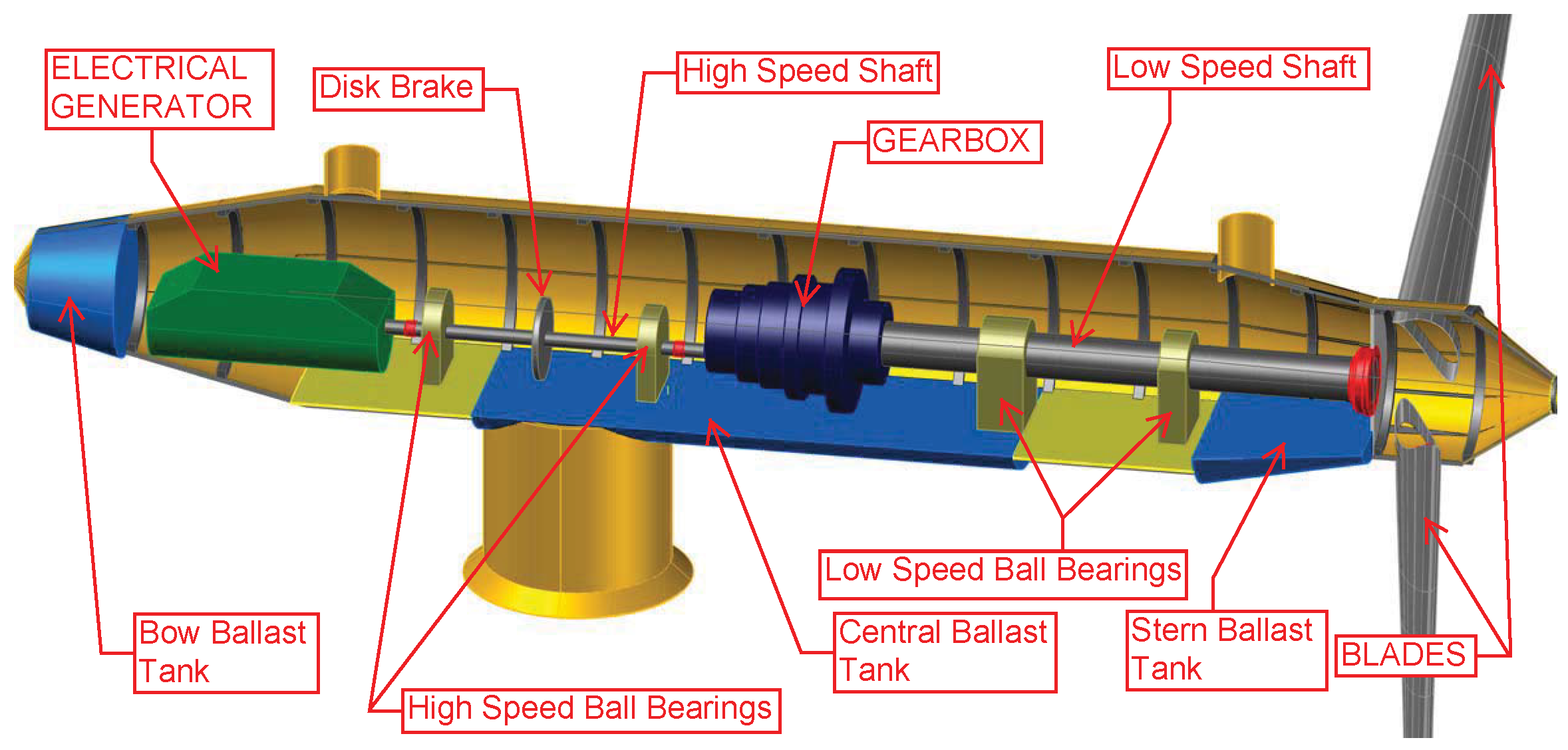
The first generation TEC presented in this work was designed to be able to perform automatic emersion/immersion maneuvers. This procedure is accomplished by controlling the inner ballast water inside the device and with the help of small guide wires. Figure 5 illustrates the distribution equipment of the proposed TEC. In this figure, it is possible to observe that the gearbox, which is responsible for converting the low speed rotor motion into the high rotational speed required by the generator to produce electricity, is located after the rotor, which converts the tidal energy into a rotary mechanical movement. A low speed and elongated high torque axis connects the rotor to the gear, while a high speed and low torque axis (also elongated) connects the gear to the generator. Other equipment, such as a brake system, electronic converters, lubrication, cooling, heating, light protection, etc., can also be considered. In order to achieve depth control operations, the design of the nacelle must include the following modifications: (a) the location of the ballast tanks and the associated pumping system; and (b) the modification of the shape of the nacelle in order to obtain neutral buoyancy when the ballast tanks are 50% full. Figure 5 shows that the nacelle has been longitudinally elongated rather than increasing its diameter in order to reduce the hydrodynamic performance as little as possible (see the two hatchways located on the upper part of the nacelle, used to gain access to the device) [25].

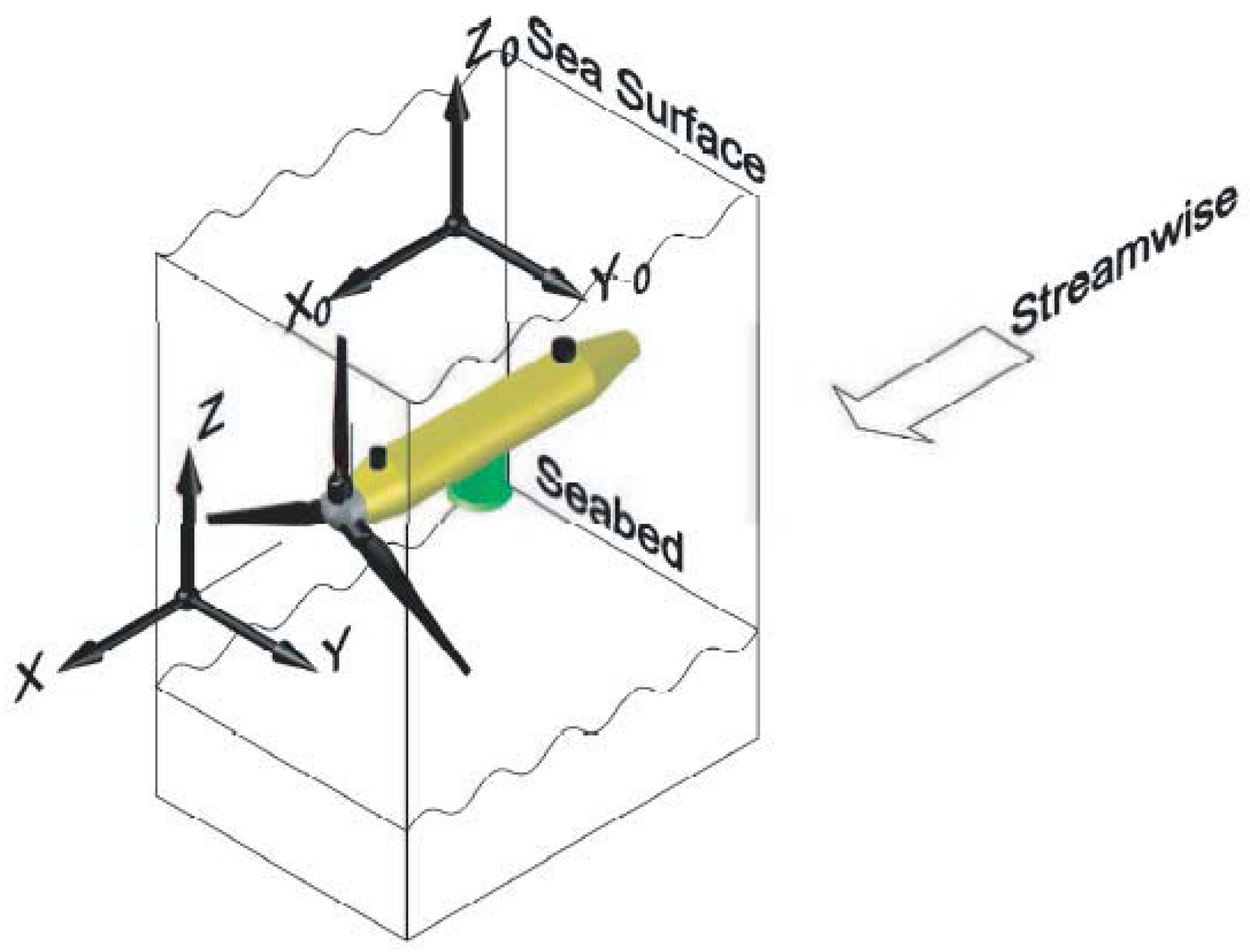
The derivation of the dynamic model of the first generation TEC plays an important role in the analysis of the behavior of the device itself, the design of control algorithms and the generation of optimized trajectories. The dynamic model chosen must be sufficiently precise to describe the behavior of the device and sufficiently simple to be included in the control law. As a previous step toward defining the dynamic model of the TEC, it is necessary to define the necessary reference frames usually used in marine energy ([30]). A fixed reference frame $\left\{S_0\right\}$ is used to represent the position and orientation of the TEC, which is referred to as a local reference frame $\left\{S\right\}$ (see Figure 6). The device coordinates are defined with regard to the fixed reference frame $\left\{S_0\right\}$, in which the x-axis is perpendicular to the rotor plane, horizontal and follows the streamwise direction; the z-axis is vertical and points upwards; and the y-axis must form a right-handed system with regard to the x,z-axis. The origin of the frame $\left\{S_0\right\}$ is located over the vertical part of the device and at the nominal level of the sea.

A practical TEC dynamic model is obtained by joining the propeller to an approximately cylindrical body on which the mechanical-electrical devices are installed. These kinds of bodies can therefore be considered to be formed of approximately cylindrical shapes. The system is provided with two degrees of freedom of movement, the depth, $z\left(t\right)$, and the rotation about the y-axis, $\theta \left(t\right)$. 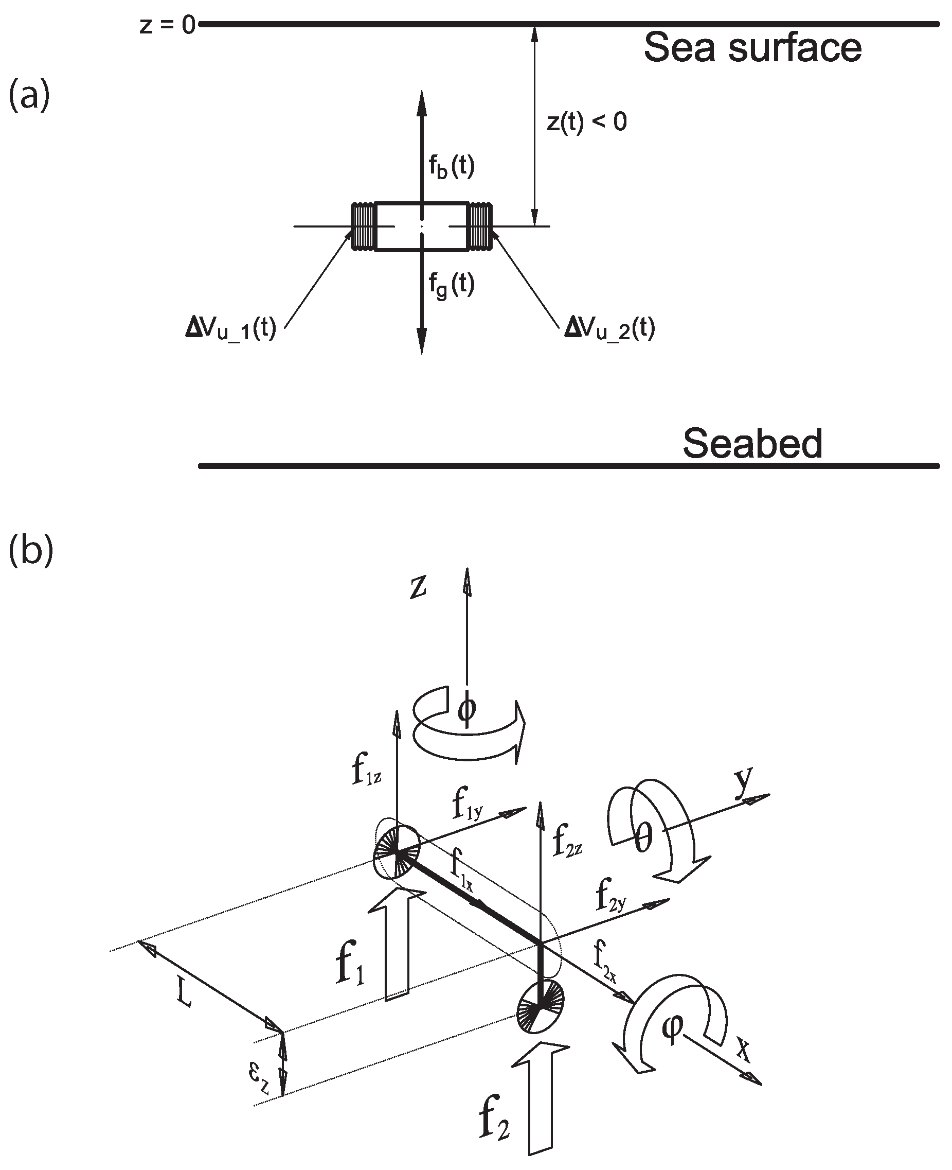Figure 7a provides a schematics representation of the main magnitudes involved in a cylindrical body to be modeled when the actuators used to produce vertical forces are conceived of as volume-increasing devices. The TEC is assumed to be composed of two lumped masses at each of the ends of the device ($m=m_1+m_2$). From the perspective of device construction, the mass distribution should be such that it ensures the stability of the body during a horizontal buoyancy state, and the application points of the forces will be slightly offset from the geometric symmetry points. Figure 7b depicts the arrangement of the two masses, the hydrostatic forces applied and the criterion of signs used in the definition of displacements and rotations. In order to achieve cylinder stability around the free-surface under buoyancy conditions, the device’s center of gravity must lie below its center of buoyancy, thereby avoiding undesired rotations about the x-axis. This settling is made possible by the arrangement of the device’s internal elements. The displacement is relatively small (${ϵ}_z⪆0$ in comparison with the cylinder diameter) and is modeled as a vertical displacement of one of the two masses (in our case, the mass $m_2$), in order to illustrate the above effect together with the non-perfect compensation of the inertia from the x-axis.

The procedure used to obtain the dynamic model is based on the expected decoupling between the translational dynamics (only the z-components) and the rotational dynamics (only the θ-components with regard to the y-axis). We first achieve the equations of motion of the vertical movement, and we then develop the rotational dynamics of the center of buoyancy. The vertical translational dynamics model is therefore obtained as follows:

$$\left(m_1+m_2+m_{Add}\right)\ddot{z}+{\nu }_z·sign\left(\dot{z}\right)·{\dot{z}}^2=f_g+f_b$$

(1)

where subindex $i=1,2$ represents the number of mass at which each of the actuators is placed, while $m_{Add}=m_{Add}(z\left(t\right),\theta \left(t\right))$ expresses the added masses of the body. We propose that these parameters be considered as a function of depth $z\left(t\right)$ (geometrical center of the proposed cylinder shape) and cylinder orientation, $\theta \left(t\right)$, by ignoring their dependence on speed, unlike that which usually occurs. The coefficient ${\nu }_z$ denotes the friction coefficient, and $f_g$ and $f_b$ are the only forces applied to the body, in the absence of other external forces, such as those from marine currents, waves, wind effects or others, all of which are considered here to be external disturbances. All forces and parameters are computed as:

$$\begin{array}{ccc}\hfill f_{ig}& =& -m_i·g\hfill \\ \hfill f_{ib}& =& V_i\left(t\right)·{\rho }_w·g\hfill \\ \hfill V_i\left(t\right)& =& {\displaystyle \frac{1}{2}·\left[V_0+V_{Compr}\left(t\right)\right]-V_{Buoy\_i}\left(t\right)+\Delta V_{u\_i}\left(t\right)}\hfill \\ \hfill V_{Buoy\_i}\left(t\right)& =& V_{Buoy\_i}(z\left(t\right),\theta \left(t\right))\hfill \\ \hfill V_{Compr}\left(t\right)& =& {\gamma }_0·z\left(t\right)\hfill \end{array}$$

(2)

where $f_g=f_{1g}+f_{2g}$ is the force of gravity, $f_b=f_{1b}+f_{2b}$ represents the buoyancy force, g is the gravity constant and $V_i\left(t\right)$ denotes the submerged volumes. Since actuators will produce variations in volume, they are considered as time-dependent variables. $V_0$ represents the nominal volume of the body outside the sea (without compression effects) and is assumed to be constant, while $V_{Buoy\_i}$ denotes the i-th fraction of the loss of buoyancy for each mass when the body is not fully submerged. It can be observed that while the cylinder always remains fully submerged, a fraction of the blades’ volume emerges from the sea in the neighborhood of the sea surface. This loss of buoyancy is not computed in the proposed dynamic model, but is rather computed as an external disturbance. ${\gamma }_0$ is the cylinder compressibility coefficient; it is constant and positive and is considered only for negative values of depth $z\left(t\right)$ (zero when the device is not submerged). $\Delta V_{u\_i}\left(t\right)$ represents the control volumes. These are actuated from servos based on motor-reduction gear-spindles and a set of linear pistons. $V_{Compr}\left(t\right)$ expresses the loss of volume owing to compressibility effects, while ${\rho }_w$ is the water density, which is considered to be constant (not as a function of depth, temperature or salinity). Note that, in the case of perfect neutral buoyancy, $m_1+m_2={\rho }_W·V_0$ and each of the forces produced by the actuators are $f_i={\rho }_w·g·\Delta V_{u\_i}$ for $i=1,2$.

Furthermore, in order to obtain the rotational dynamics, it is necessary to obtain operation conditions that will force the TEC to be at an equilibrium point. Under neutral buoyancy, the rotational dynamics is the following:

$$\left(I_{yy}+I_{yy\_Add}\right)\ddot{\theta }+{\nu }_{\theta }·sign(\dot{\theta }){\dot{\theta }}^2=(f_1-f_2)\frac{L{C}_{\theta }}{2}+f_2{ϵ}_z{S}_{\theta }$$

(3)

$${\displaystyle I_{yy}=\left(m_1+m_2\right)\frac{L^2}{4}+m_2{ϵ}_z^2}$$

(4)

where $S_{\theta }\equiv sin\theta$, $C_{\theta }\equiv cos\theta$, $I_{yy}$ is the moment of inertia about the y-axis of rotation, $I_{yy\_Add}$ represents the effect of the added masses on the rotational dynamics, ${\nu }_{\theta }$ denotes the friction coefficient, L is the length of the nominal cylinder outside the sea (without compression effects) and ${ϵ}_z$ expresses the offset distance shown in Figure 7b. From the point of view of force generation, the decoupled movements are therefore easily obtained as:

• Only translational movements: $f_1=f_2$ ⇒ $f_z=f_1+f_2$ and ${\mathsf{\Gamma }}_y=f_2{ϵ}_z{S}_{\theta }\approx 0$.
• Only rotational movements: $f_1=-f_2$ ⇒ $f_z=0$ and ${\mathsf{\Gamma }}_y=(f_1-f_2)\frac{L{C}_{\theta }}{2}+f_2{ϵ}_z{S}_{\theta }$.
• Equilibrium movement: $f_1=f_2=0$ ⇒ $f_z=0$ and ${\mathsf{\Gamma }}_y=0$.

Finally, it is necessary to define the input transformation matrix between the uncoupled set of force $f_z$ and torque ${\mathsf{\Gamma }}_y$ and the control volumes $\Delta V_{u\_i}\left(t\right)$ for $i=1,2$. This relationship is provided by means of the following expression:

$$\underset{\mathsf{\Xi }}{\underbrace{\left[\begin{array}{c}{f}_z\\ {\mathsf{\Gamma }}_y\end{array}\right]}}=\underset{\mathbf{M}\left(\mathbf{q}\right)}{\underbrace{\left[\begin{array}{cc}1& 1\\ \frac{L{C}_{\theta }}{2}& -\frac{L{C}_{\theta }}{2}+{ϵ}_z{S}_{\theta }\end{array}\right]}}·\underset{\mathbf{F}}{\underbrace{{\rho }_W·g·\left[\begin{array}{c}\Delta V_{u\_1}\\ \Delta V_{u\_2}\end{array}\right]}}$$

(5)

Note that the input vector Ξ can provide arbitrary values because this model considers the combined movements of vertical translation and rotation. It will be observed that matrix $\mathbf{M}$ is invertible for all of the desired range of $-\pi /2\le \theta \le 0$ $rad$ owing to the small displacement ${ϵ}_z$ included in the model and depicted in Figure 7b. If the compressibility effects are ignored here, all of the movements (both uncoupled or coupled) can be achieved as:

• Only translational movements: $\mathsf{\Xi }={\left[\begin{array}{cc}{f}_z& 0\end{array}\right]}^T$.
• Only rotational movements: $\mathsf{\Xi }={\left[\begin{array}{cc}0& {\mathsf{\Gamma }}_y\end{array}\right]}^T$.
• Simultaneous movements: $\mathsf{\Xi }={\left[\begin{array}{cc}{f}_z& {\mathsf{\Gamma }}_y\end{array}\right]}^T$.
• Equilibrium movement: $\mathsf{\Xi }={\left[\begin{array}{cc}0& 0\end{array}\right]}^T$.

Finally, the dynamic model is expressed in matrix form as follows (where $\mathbf{q}\left(t\right)={\left[\begin{array}{cc}z\left(t\right)& \theta \left(t\right)\end{array}\right]}^T$):

$$\begin{array}{ccc}\hfill & & \underset{\mathbf{B}}{\underbrace{\left[\begin{array}{cc}\left(m_1+m_2+m_{Add}\right)& 0\\ 0& \left(I_{yy}+I_{yy\_Add}\right)\end{array}\right]}}·\underset{\ddot{\mathbf{q}}}{\underbrace{\left[\begin{array}{c}\ddot{z}\\ \ddot{\theta }\end{array}\right]}}+\underset{\mathbf{V}(\mathbf{q},\dot{\mathbf{q}})}{\underbrace{\left[\begin{array}{c}{\nu }_z·sign(\dot{z})·{\dot{z}}^2\\ {\nu }_{\theta }·sign(\dot{\theta })·{\dot{\theta }}^2\end{array}\right]-\left[\begin{array}{cc}{\gamma }_0& 0\\ 0& 0\end{array}\right]·\left[\begin{array}{c}z\\ \theta \end{array}\right]}}\hfill \\ & & =\underset{\mathbf{M}\left(\mathbf{q}\right)}{\underbrace{\left[\begin{array}{cc}1& 1\\ \frac{L{C}_{\theta }}{2}& -\frac{L{C}_{\theta }}{2}+{ϵ}_z{S}_{\theta }\end{array}\right]}}·\underset{\mathbf{F}}{\underbrace{{\rho }_W·g·\left[\begin{array}{c}\Delta V_{u\_1}\\ \Delta V_{u\_2}\end{array}\right]}}\hfill \end{array}$$

(6)

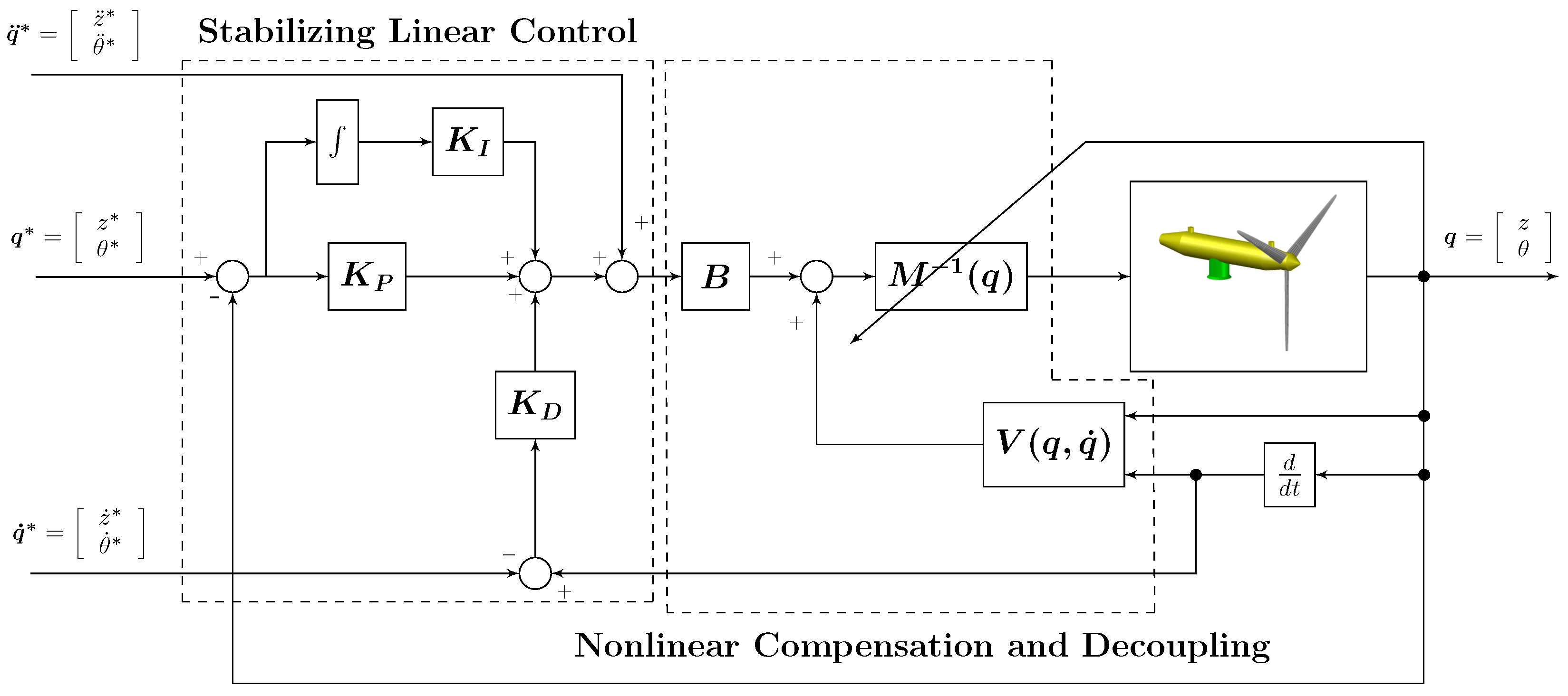
3. General Control Scheme

Figure 8 illustrates the general scheme proposed for the control of the two degrees of freedom first generation TEC. Let us suppose that a desired trajectory is provided for the depth, $z\left(t\right)$, and the rotation about the y-axis, $\theta \left(t\right)$, in the form of specified time functions: $z^{*}\left(t\right)$ and ${\theta }^{*}\left(t\right)$, respectively. A nonlinear feedback controller is used to accomplish the tracking of the given desired controlled variables, $\mathbf{q}\left(t\right)={[z\left(t\right),\theta \left(t\right)]}^T$, which is given by:

$$\begin{array}{c}\hfill \mathbf{F}\left(t\right)={\mathbf{M}}^{-1}\left(\mathbf{q}\left(\mathbf{t}\right)\right)·\left[\mathbf{B}·\mathsf{\Gamma }\left(t\right)+\mathbf{V}(\mathbf{q}\left(t\right),\dot{\mathbf{q}}\left(t\right))\right]\end{array}$$

(7)

in which the auxiliary control input $\mathsf{\Gamma }\left(t\right)$ is synthesized as follows:

$$\begin{array}{c}\hfill \mathsf{\Gamma }\left(t\right)=\ddot{{\mathbf{q}}^{*}}\left(t\right)-{\mathbf{K}}_{\mathbf{D}}\left[\dot{\mathbf{q}}\left(t\right)-\dot{{\mathbf{q}}^{*}}\left(t\right)\right]-{\mathbf{K}}_{\mathbf{P}}\left[\mathbf{q}\left(t\right)-{\mathbf{q}}^{*}\left(t\right)\right]-{\mathbf{K}}_{\mathbf{I}}\int \left[\mathbf{q}\left(\tau \right)-{\mathbf{q}}^{*}\left(\tau \right)\right]d\tau \end{array}$$

(8)

where ${\mathbf{K}}_{\mathbf{P}}$, ${\mathbf{K}}_{\mathbf{I}}$ and ${\mathbf{K}}_{\mathbf{D}}$ $\in {\mathbb{R}}^{2\times 2}$ are the diagonal positive definite matrices that represent the design elements of a vector-valued classical multivariable proportional-integral-derivative (PID) controller. As can be observed in Figure 8, the control scheme is composed of an inner loop based on the dynamic model of the first generation TEC and an outer loop based on a stabilizing linear control action, which operates with the tracking error vector ${\mathbf{e}}_{\mathbf{q}}\left(t\right)=\mathbf{q}\left(t\right)-{\mathbf{q}}^{*}\left(t\right)$. The main objective of the inner loop is to obtain a linear and decoupled input/output relationship, and this requires the computation of the matrix that relates the control volumes, $\Delta V_{u\_i}\left(t\right)$ for $i=1,2$, and the uncoupled set of force $f_z$ and torque ${\mathsf{\Gamma }}_y$, i.e., ${\mathbf{M}}^{-1}\left(\mathbf{q}\right)$; the inertia matrix $\mathbf{B}$ and the vector of friction and compressibility terms $\mathbf{V}(\mathbf{q},\dot{\mathbf{q}})$. Two of these terms, ${\mathbf{M}}^{-1}\left(\mathbf{q}\left(t\right)\right)$ and $\mathbf{V}(\mathbf{q}\left(t\right),\dot{\mathbf{q}}\left(t\right))$, need to be computed online owing to the fact that the matrices of which this feedback loop is composed depend on the current values of the system dynamics $\mathbf{q}\left(t\right)$ and $\dot{\mathbf{q}}\left(t\right)$. Furthermore, the main objective of the outer loop is to stabilize the overall system. This part of the controller design is highly simplified since it operates an uncoupled $2\times 2$ multivariable time-invariant system.

The dynamics of the closed loop tracking error vector, ${\mathbf{e}}_{\mathbf{q}}\left(t\right)=\mathbf{q}\left(t\right)-{\mathbf{q}}^{*}\left(t\right)={[z\left(t\right)-z^{*}\left(t\right);\theta \left(t\right)-{\theta }^{*}\left(t\right)]}^T$, for the control of the first generation TEC is obtained after substituting Expressions (7) and (8) in (6), yielding the following expression:

$$\begin{array}{c}\hfill \ddot{\mathbf{q}}=\ddot{{\mathbf{q}}^{*}}\left(t\right)-{\mathbf{K}}_{\mathbf{D}}\left[\dot{\mathbf{q}}\left(t\right)-\dot{{\mathbf{q}}^{*}}\left(t\right)\right]-{\mathbf{K}}_{\mathbf{P}}\left[\mathbf{q}\left(t\right)-{\mathbf{q}}^{*}\left(t\right)\right]-{\mathbf{K}}_{\mathbf{I}}\int \left[\mathbf{q}\left(\tau \right)-{\mathbf{q}}^{*}\left(\tau \right)\right]d\tau \end{array}$$

(9)

In this case, the closed loop tracking error, ${\mathbf{e}}_{\mathbf{q}}\left(t\right)=\mathbf{q}\left(t\right)-{\mathbf{q}}^{*}\left(t\right)$, evolves governed by the following third order $2\times 2$ differential equation:

$$\begin{array}{c}\hfill {\mathbf{e}}_{\mathbf{q}}^{\left(\mathbf{3}\right)}\left(t\right)+{\mathbf{K}}_{\mathbf{D}}{\ddot{\mathbf{e}}}_{\mathbf{q}}\left(t\right)+{\mathbf{K}}_{\mathbf{P}}{\dot{\mathbf{e}}}_{\mathbf{q}}\left(t\right)+{\mathbf{K}}_{\mathbf{I}}{\mathbf{e}}_{\mathbf{q}}\left(t\right)=0\end{array}$$

(10)

whose trajectories, and of their time derivatives, therefore converge, in an asymptotically exponentially-dominated manner onto a small as desired neighborhood of the origin of the phase space of the tracking error vector, depending on the design matrices $\{{\mathbf{K}}_{\mathbf{P}},{\mathbf{K}}_{\mathbf{I}},{\mathbf{K}}_{\mathbf{D}}\}$ selected. The controller design matrices $\{{\mathbf{K}}_{\mathbf{P}},{\mathbf{K}}_{\mathbf{I}},{\mathbf{K}}_{\mathbf{D}}\}$ must be designed so as to render the following $2\times 2$ complex valued diagonal matrix, $\mathbf{p}\left(s\right)$, defined as:

$$\mathbf{p}\left(s\right)={\mathbf{I}}^{2\times 2}{s}^3+{\mathbf{K}}_{\mathbf{D}}{s}^2+{\mathbf{K}}_{\mathbf{P}}s+{\mathbf{K}}_{\mathbf{I}}=0$$

(11)

as third degree Hurwitz polynomials with desirable root locations. The stability of Expression (10) can be easily studied by using the Routh–Hurwitz criterion. Bearing in mind that the set of design matrices $\{{\mathbf{K}}_{\mathbf{P}},{\mathbf{K}}_{\mathbf{I}},{\mathbf{K}}_{\mathbf{D}}\}$ is diagonal, the stability of each error variable ${\mathbf{e}}_{\mathbf{q}}\left(t\right)={[e_z\left(t\right);e_{\theta }\left(t\right)]}^T={[z\left(t\right)-z^{*}\left(t\right);\theta \left(t\right)-{\theta }^{*}\left(t\right)]}^T$, can be studied in an independent manner. After applying the Routh–Hurwitz criterion, the following stability conditions: (i) $K_{D_i},K_{P_i}>0$ and; (ii) $0<K_{I_i}<K_{D_i}{K}_{P_i}$ are obtained for $i=z,\theta$. After considering the previous stability restrictions, the constant controller gain matrices $\{{\mathbf{K}}_{\mathbf{P}},{\mathbf{K}}_{\mathbf{I}},{\mathbf{K}}_{\mathbf{D}}\}$ were chosen so as to obtain the following desired closed-loop characteristic $2\times 2$ complex valued diagonal matrix:

$${\mathbf{p}}^{\mathbf{des}}\left(s\right)=\left({\mathbf{I}}^{2\times 2}{s}^2+2{\mathbf{\zeta }}_{\mathbf{c}}{\mathbf{\omega }}_{\mathbf{c}}s+{\left({\mathbf{\omega }}_{\mathbf{c}}\right)}^2\right)·\left({\mathbf{I}}^{2\times 2}s+{\mathbf{p}}_{\mathbf{c}}\right)$$

(12)

where ${\mathbf{\zeta }}_{\mathbf{c}}$, ${\mathbf{\omega }}_{\mathbf{c}}$ and ${\mathbf{p}}_{\mathbf{c}}$ $\in {\mathbb{R}}^{2\times 2}$ are diagonal positive definite matrices. The values of the constant controller gain matrices are obtained directly by identifying each term in Expression (11) with those of (12). The gain matrices $\{{\mathbf{K}}_{\mathbf{P}},{\mathbf{K}}_{\mathbf{I}},{\mathbf{K}}_{\mathbf{D}}\}$ of the proposed nonlinear controller were then set to be:

$$\begin{array}{ccc}\hfill {\mathbf{K}}_{\mathbf{D}}& =& 2{\mathbf{\zeta }}_{\mathbf{c}}{\mathbf{\omega }}_{\mathbf{c}}+{\mathbf{p}}_{\mathbf{c}}\hfill \\ \hfill {\mathbf{K}}_{\mathbf{P}}& =& {\left({\mathbf{\omega }}_{\mathbf{c}}\right)}^2+2{\mathbf{\zeta }}_{\mathbf{c}}{\mathbf{\omega }}_{\mathbf{c}}{\mathbf{p}}_{\mathbf{c}}\hfill \\ \hfill {\mathbf{K}}_{\mathbf{I}}& =& {\left({\mathbf{\omega }}_{\mathbf{c}}\right)}^2{\mathbf{p}}_{\mathbf{c}}\hfill \end{array}$$

(13)

4. Numerical Simulations

Numerical simulations were carried out in order to verify that the above designed controller performs very well in terms of generator controllability, ability to perform emersion and immersion maneuvers with only passive buoyancy forces, quick convergence of the tracking errors onto a small neighborhood of zero, smooth transient responses, low control effort and robustness in the case of model parametric uncertainties. The values of the physical parameters of the first generation TEC used in the simulations were: $m_1=m_2=$ 38,545 kg, $m_{Add}$ = 55,119 kg, $L=16.8$ m, ${\rho }_W=1025$ kg/m${}^3$, $g=9.81$ m/s${}^2$, $I_{yy}=$ 5,439,470.4 kg·m${}^2$, $I_{yy\_Add}=$ 3,889,197 kg·m${}^2$, ${\nu }_z=$ 24,830 kg/m, ${\nu }_{\theta }=$ 18,204 kg·m and ${ϵ}_z=0.1$ m. The values of $m_{Add}$, $I_{yy\_Add}$, ${\nu }_z$ and ${\nu }_{\theta }$ were obtained based on the cylindrical shape of the device and for Reynolds values lower than ${10}^5$ [31]. Some discrepancies in the controller parameters have been also included owing to the difficulty involved in adequately modeling all of the dynamics terms. In particular, errors of 10% have been inserted into all terms of which the matrices $\mathbf{M}\left(\mathbf{q}\right(t\left)\right)$ and $\mathbf{V}(\mathbf{q}\left(t\right),\dot{\mathbf{q}}\left(t\right))$ are composed. All gain vectors were tuned according to the procedure explained in Section 3 by using Equations (11)–(13) and by considering pure real roots and taking into consideration the performance of the tracking error vector ${\mathbf{e}}_{\mathbf{q}}\left(t\right)$. The values of the matrices of the desired Hurwitz polynomial vector for the feedback controller were set as ${\mathbf{\zeta }}_{\mathbf{c}}=diag(1.2,1.2)$, ${\mathbf{\omega }}_{\mathbf{c}}=diag(0.15,0.15)$ and ${\mathbf{p}}_{\mathbf{c}}=diag(2,2)$. The simulations were performed in the MATLAB/Simulink^® software environment, using the Runge–Kutta method with a fixed time sampling of $0.2$ s. Finally, the proposed dynamic model and the nonlinear control were evaluated when the TEC performed emersion maneuvers for general maintenance tasks, such as oil changes, the lubrication of gears and bearings, filter and brake pad replacement, pump and battery reviews, etc., all of which require technical staff to access the nacelle, and emersion maneuvers for blade-cleaning maintenance tasks over the sea surface. In both cases, a time window with a good weather forecast, where the influence of the waves is negligible (with maximum ranges between 0.5 and 1 m), is required. This is dealt with in the following subsections.

4.1. General Maintenance Tasks in the Nacelle

The minimal requirement needed to obtain the depth and orientation controlled device is the capability to move from a given initial posture to a desired final posture. The saturation of the actuators used to produce vertical forces limits the possibility of carrying out emersion/immersion maneuvers in response to single reference signals, such as step signals, among others. A trajectory is therefore defined as a time history of depth, speed and higher order time derivatives of the desired motion of the device [32,33]. In this simulation, it is desirable to maintain the orientation of the TEC in its null value and to track a synchronous blended polynomial type trajectory for the depth, which is frequently adopted in industrial practice. In particular, a trapezoidal velocity profile is assigned, which imposes a constant acceleration in the start phase, a cruise velocity and a constant deceleration in the arrival phase. The trajectory is therefore composed of a linear segment connected by two parabolic segments to the initial and final positions [34]. The following sequence of polynomials is generated for the construction of the desired trajectory of the depth variable:

$$z^{*}\left(t\right)=\left\{\begin{array}{l}{z}_{d_i}\mathrm{for}0\le t\le t_{0_z}\\ z_{d_i}+\frac{1}{2}{\ddot{z}}_c{(t_{f_z}-t_{0_z})}^2\mathrm{for}{t}_{0_z}\le t\le t_{0_z}+t_{c_z}\\ z_{d_i}+{\ddot{z}}_c{t}_{c_z}(t-t_{0_z}-\frac{t_{c_z}}{2})\mathrm{for}{t}_{c_z}+t_{0_z}\le t\le t_{f_z}-t_{c_z}+t_{0_z}\\ z_{d_f}-\frac{1}{2}{\ddot{z}}_c{(t_{f_z}-t+t_{0_z})}^2\mathrm{for}{t}_{f_z}-t_{c_z}+t_{0_z}\le t\le t_{f_z}+t_{0_z}\\ z_{d_f}\mathrm{for}t\ge t_{f_z}+t_{0_z}\end{array}\right.$$

(14)

where $z_{d_i}=-40$ $\left[m\right]$, $z_{d_f}=-1$ $\left[m\right]$, $t_{0_z}=75$ $\left[s\right]$, $t_{f_z}=525$ $\left[s\right]$ and the values of $t_{c_z}$ and ${\ddot{z}}_c$ are obtained as:

$$\begin{array}{ccc}\hfill {\ddot{z}}_c& =& 8\frac{(z_{d_f}-z_{d_i})}{{(t_{f_z}-t_{0_z})}^2}\hfill \end{array}$$

(15)

$$\begin{array}{ccc}\hfill t_{c_z}& =& \frac{(t_{f_z}-t_{0_z})}{2}-\frac{1}{2}\sqrt{\frac{{(t_{f_z}-t_{0_z})}^2{\ddot{z}}_c-4(z_{d_f}-z_{d_i})}{{\ddot{z}}_c}}\hfill \end{array}$$

(16)

The evolution of the dynamic states of the nonlinear system obtained for each of the independent movements of the TEC is shown in Figure 9. It will be observed that the system performs extremely well with the desired settling time and with no overshoot. This figure also shows that the nacelle is always fully submerged and that no free-surface interaction occurs when a fraction of the propeller remains outside the sea. 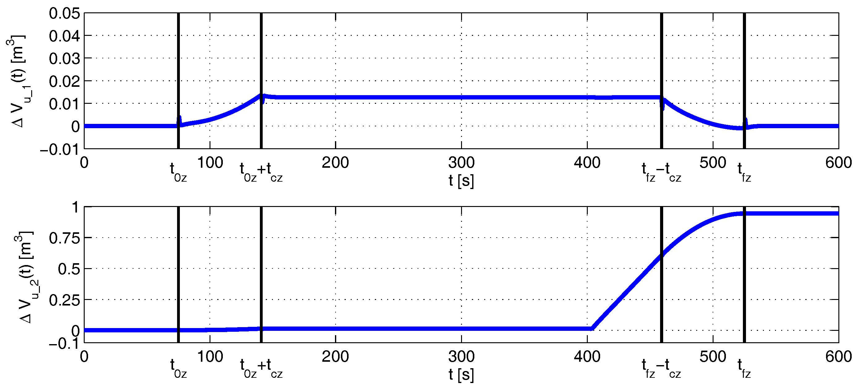Figure 10 illustrates the evolution of the input control volumes of the system in charge of producing the adequate vertical forces that permit the control of the depth and the orientation of the device, even when part of the propeller moves out of the water causing a loss of buoyancy ($V_{buoy\_2}\ne 0$; see Equation (2)). This is computed in the dynamic model as an external disturbance. Figure 10 shows how the controller generates adequate control signals that compensate for the aforementioned loss of buoyancy applied in the neighborhood of mass $m_2$. 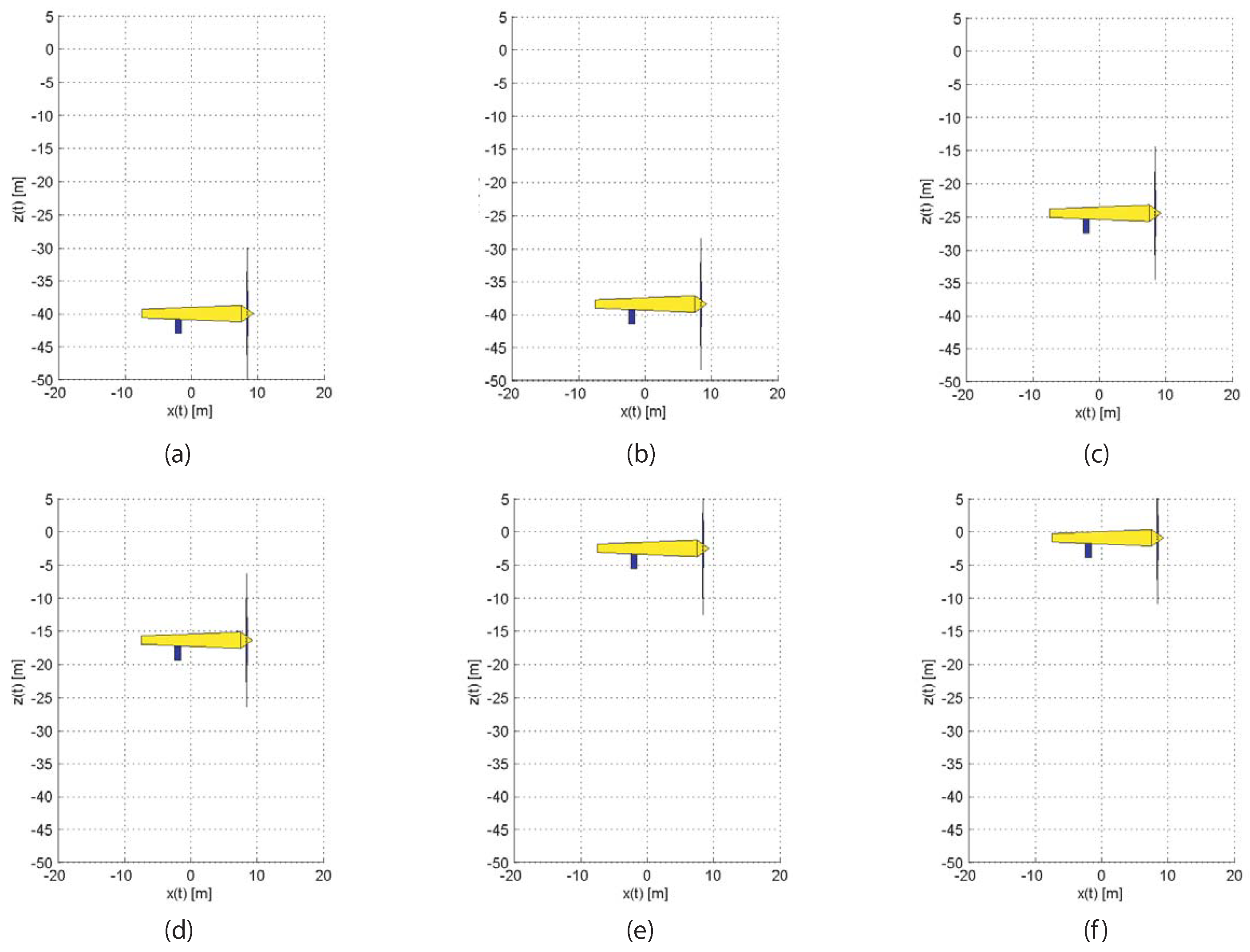A very small error of less than $0.1^{\circ }$ in the orientation tracking caused by this disturbance can be appreciated in Figure 9. Finally, a visual snapshot of the sequence performed is illustrated in Figure 11, which shows that the orientation of the device is continuously maintained near its null value, despite the nonlinear loss of buoyancy caused by the propeller.

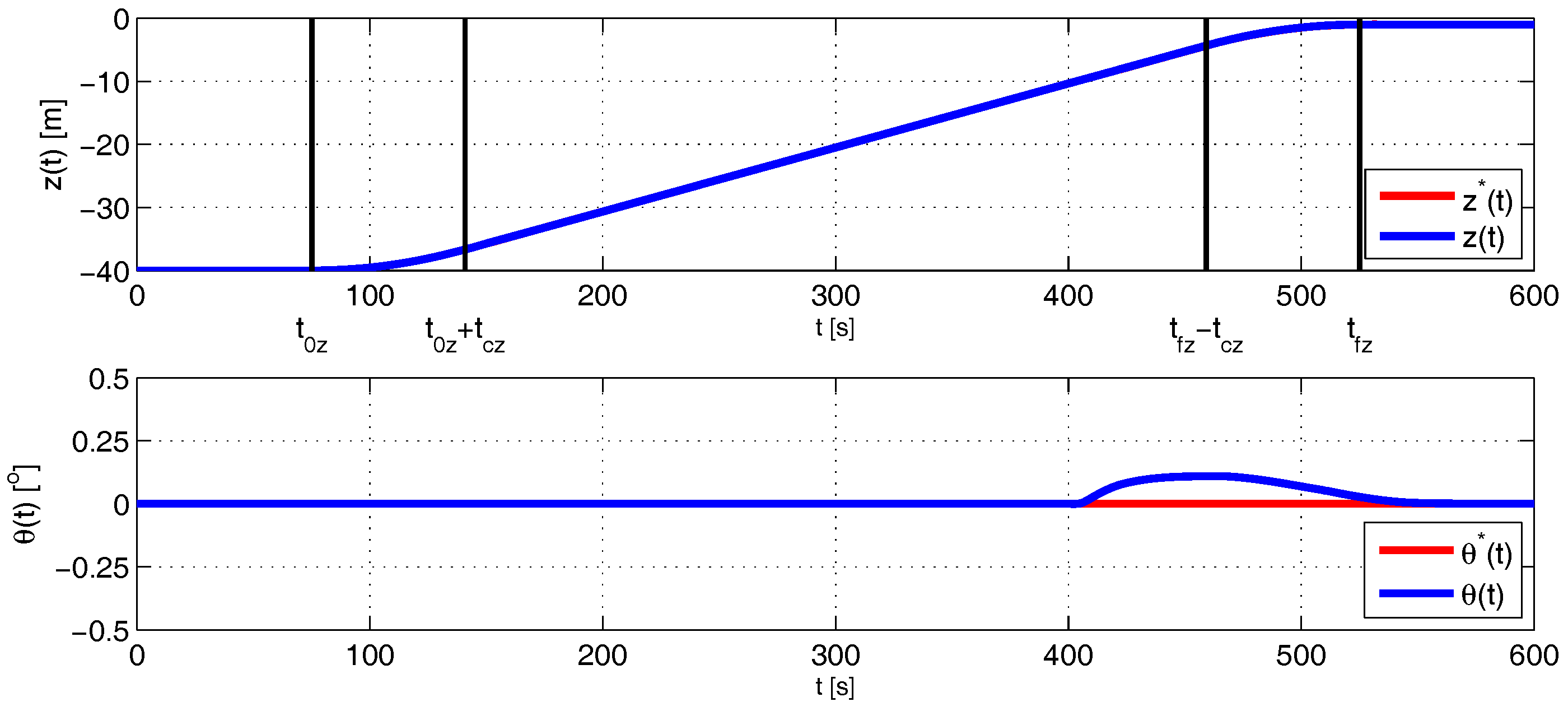
4.2. Blade-Cleaning Maintenance Tasks

In this case, in order to perform blade-cleaning maintenance tasks, it is necessary to design a linear segment connected by two parabolic segments to the initial and final positions for both the depth and orientation variables. The following sequence of polynomials is generated for each of the controlled variables:

$${\theta }^{*}\left(t\right)=\left\{\begin{array}{c}{\theta }_{d_i}\mathrm{for}0\le t\le t_{0_{\theta }}\hfill \\ {\theta }_{d_i}+\frac{1}{2}{\ddot{\theta }}_c{(t_{f_{\theta }}-t_{0_{\theta }})}^2\mathrm{for}{t}_{0_{\theta }}\le t\le t_{0_{\theta }}+t_{c_{\theta }}\hfill \\ {\theta }_{d_i}+{\ddot{\theta }}_c{t}_{c_{\theta }}(t-t_{0_{\theta }}-\frac{t_{c_{\theta }}}{2})\mathrm{for}{t}_{c_{\theta }}+t_{0_{\theta }}\le t\le t_{f_{\theta }}-t_{c_{\theta }}+t_{0_{\theta }}\hfill \\ {\theta }_{d_f}-\frac{1}{2}{\ddot{\theta }}_c{(t_{f_{\theta }}-t+t_{0_{\theta }})}^2\mathrm{for}{t}_{f_{\theta }}-t_{c_{\theta }}+t_{0_{\theta }}\le t\le t_{f_{\theta }}+t_{0_{\theta }}\hfill \\ {\theta }_{d_f}\mathrm{for}t\ge t_{f_{\theta }}+t_{0_{\theta }}\hfill \end{array}\right.$$

(17)

$$z^{*}\left(t\right)=\left\{\begin{array}{c}{z}_{d_i}\mathrm{for}0\le t\le t_{0_{z1}}\hfill \\ z_{d_i}+\frac{1}{2}{\ddot{z}}_{c1}{(t_{f_{z1}}-t_{0_{z1}})}^2\mathrm{for}{t}_{0_{z1}}\le t\le t_{0_{z1}}+t_{c_{z1}}\hfill \\ z_{d_i}+{\ddot{z}}_{c1}{t}_{c_{z1}}(t-t_{0_{z1}}-\frac{t_{c_{z1}}}{2})\mathrm{for}{t}_{c_{z1}}+t_{0_{z1}}\le t\le t_{f_{z1}}-t_{c_{z1}}+t_{0_{z1}}\hfill \\ z_{d_{f1}}-\frac{1}{2}{\ddot{z}}_{c1}{(t_{f_{z1}}-t+t_{0_{z1}})}^2\mathrm{for}{t}_{f_{z1}}-t_{c_{z1}}+t_{0_{z1}}\le t\le t_{f_{z1}}+t_{0_{z1}}\hfill \\ z_{d_{f1}}\mathrm{for}{t}_{f_{z1}}+t_{0_{z1}}\ge t\ge t_{0_{z2}}\hfill \\ z_{d_{f1}}+\frac{1}{2}{\ddot{z}}_{c2}{(t_{f_{z2}}-t_{0_{z2}})}^2\mathrm{for}{t}_{0_{z2}}\le t\le t_{0_{z2}}+t_{c_{z2}}\hfill \\ z_{d_{f1}}+{\ddot{z}}_{c2}{t}_{c_{z2}}(t-t_{0_{z2}}-\frac{t_{c_{z2}}}{2})\mathrm{for}{t}_{c_{z2}}+t_{0_{z2}}\le t\le t_{f_{z2}}-t_{c_{z2}}+t_{0_{z2}}\hfill \\ z_{d_{f2}}-\frac{1}{2}{\ddot{z}}_{c2}{(t_{f_{z2}}-t+t_{0_{z2}})}^2\mathrm{for}{t}_{f_{z2}}-t_{c_{z2}}+t_{0_{z2}}\le t\le t_{f_{z2}}+t_{0_{z2}}\hfill \\ z_{d_{f2}}\mathrm{for}t\ge t_{f_{z2}}+t_{0_{z2}}\hfill \end{array}\right.$$

(18)

where ${\theta }_{d_i}=0$${}^{\circ }$, ${\theta }_{d_f}=89$${}^{\circ }$, $t_{0_{\theta }}=190$ s, $t_{f_{\theta }}=370$ s, $z_{d_i}=-40$ m, $z_{d_{f1}}=-25$ m, $t_{0_{z1}}=5$ s, $t_{f_{z1}}=155$ s, $z_{d_{f2}}=-25$ m, $z_{d_f}=-10$ m, $t_{0_{z2}}=405$ s, $t_{f_{z2}}=555$ s, and the values of $t_{c_{\theta }}$, $t_{c_z}$, ${\ddot{\theta }}_c$ and ${\ddot{z}}_c$ are obtained as:

$$\begin{array}{ccc}\hfill {\ddot{\theta }}_c& =& 8\frac{({\theta }_{d_f}-{\theta }_{d_i})}{{(t_{f_{\theta }}-t_{0_{\theta }})}^2}\hfill \end{array}$$

(19)

$$\begin{array}{ccc}\hfill {\ddot{z}}_{c1}& =& 8\frac{(z_{d_{f1}}-z_{d_i})}{{(t_{f_{z1}}-t_{0_{z1}})}^2}\hfill \end{array}$$

(20)

$$\begin{array}{ccc}\hfill {\ddot{z}}_{c2}& =& 8\frac{(z_{d_{f2}}-z_{d_{f1}})}{{(t_{f_{z2}}-t_{0_{z2}})}^2}\hfill \end{array}$$

(21)

$$\begin{array}{ccc}\hfill t_{c_{\theta }}& =& \frac{(t_{f_{\theta }}-t_{0_{\theta }})}{2}-\frac{1}{2}\sqrt{\frac{{(t_{f_{\theta }}-t_{0_{\theta }})}^2{\ddot{\theta }}_c-4({\theta }_{d_f}-{\theta }_{d_i})}{{\ddot{\theta }}_c}}\hfill \end{array}$$

(22)

$$\begin{array}{ccc}\hfill t_{c_{z1}}& =& \frac{(t_{f_{z1}}-t_{0_{z1}})}{2}-\frac{1}{2}\sqrt{\frac{{(t_{f_{z1}}-t_{0_{z1}})}^2{\ddot{z}}_{c1}-4(z_{d_{f1}}-z_{d_i})}{{\ddot{z}}_{c1}}}\hfill \end{array}$$

(23)

$$\begin{array}{ccc}\hfill t_{c_{z2}}& =& \frac{(t_{f_{z2}}-t_{0_{z2}})}{2}-\frac{1}{2}\sqrt{\frac{{(t_{f_{z2}}-t_{0_{z2}})}^2{\ddot{z}}_{c2}-4(z_{d_{f2}}-z_{d_{f1}})}{{\ddot{z}}_{c2}}}\hfill \end{array}$$

(24)

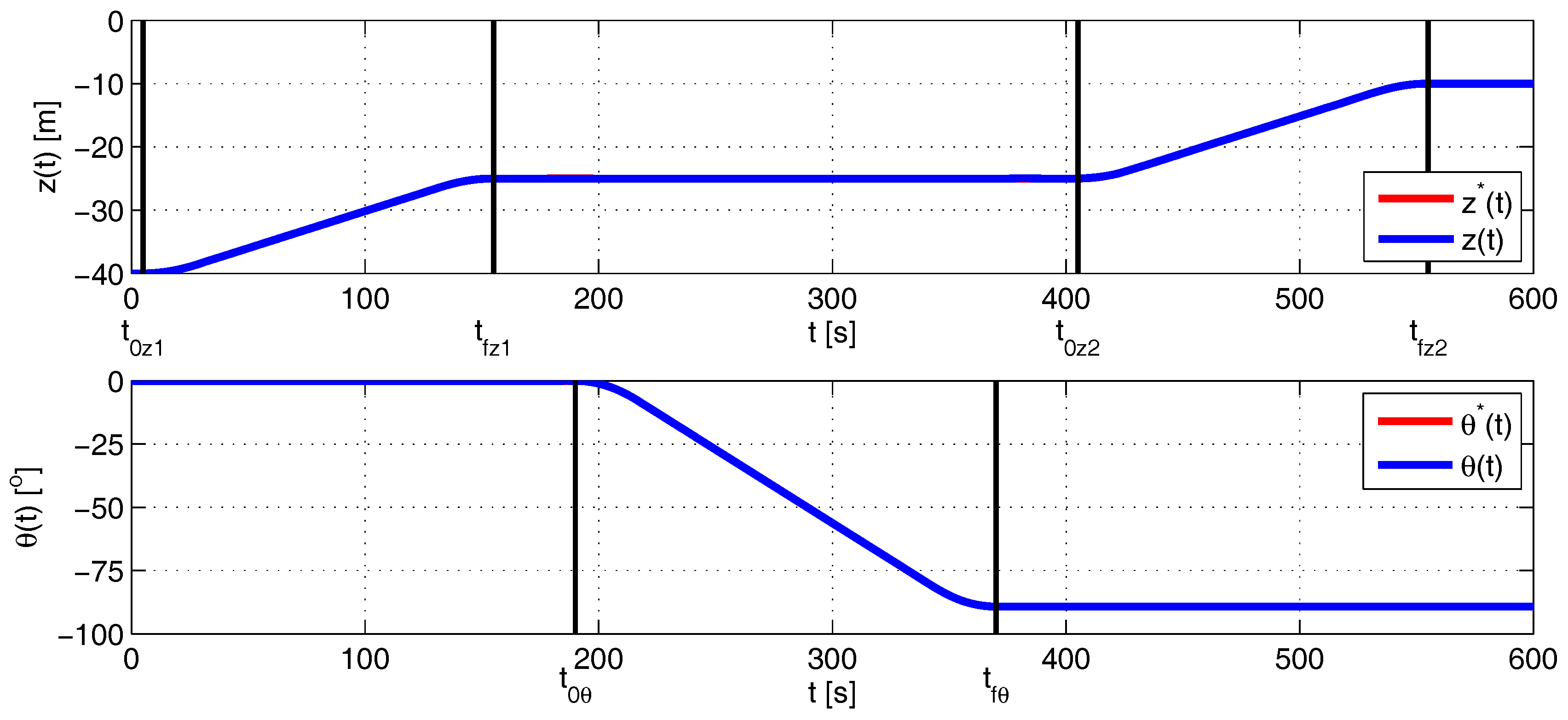
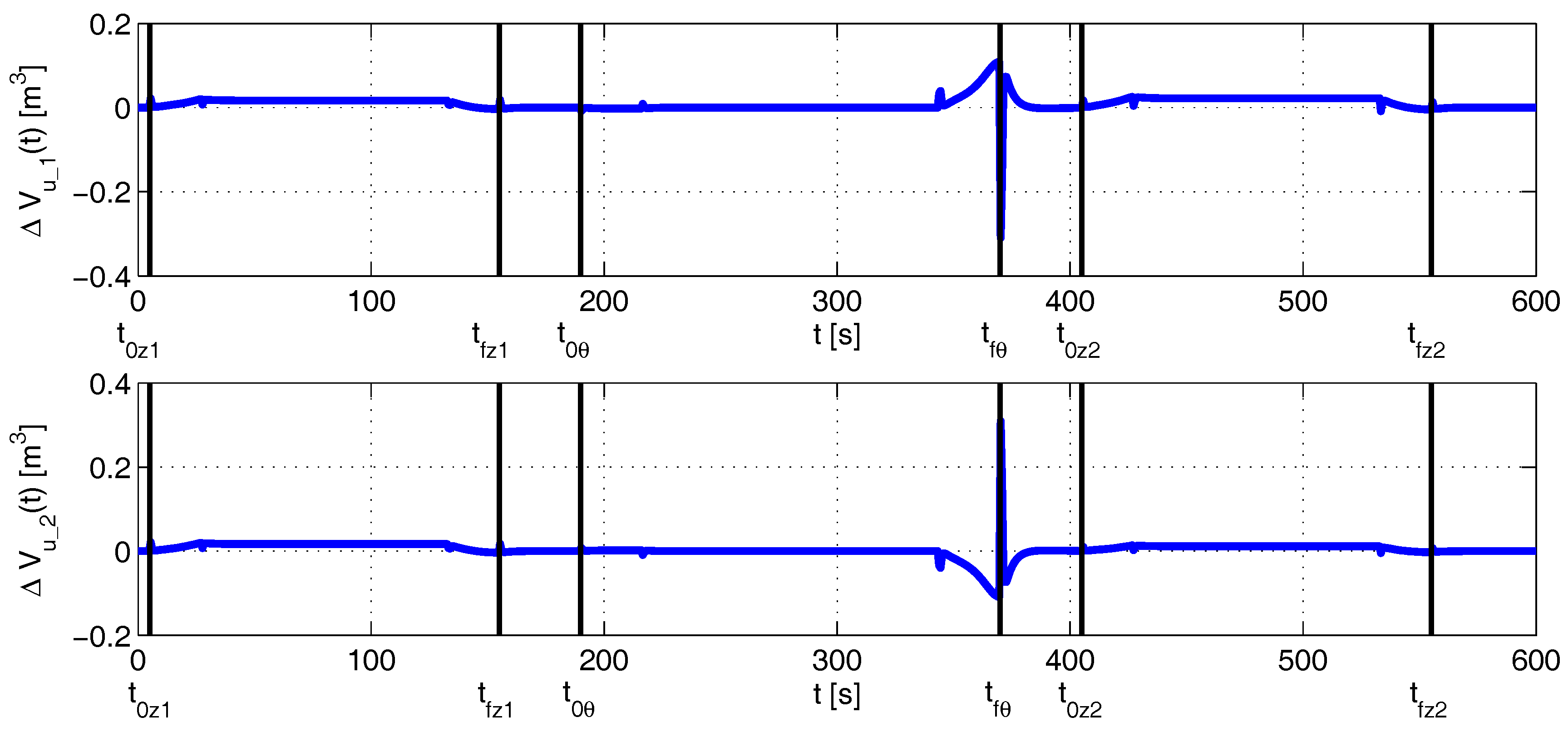
The evolution of the dynamic states of the nonlinear system obtained for each of the independent movements of the TEC is shown in Figure 12. As in the previous emersion maneuver, the system performs extremely well with the desired settling time and with no overshoot, and the device is always fully submerged, which no free-surface interaction occurs. Figure 13 illustrates the evolution of the input control volumes of the system in charge of producing the adequate vertical forces that permit the control of the depth and the orientation of the device. This figure also shows that an increase in the input control volumes is obtained when the orientation of the system is close to $-{90}^{\circ }$. The reason for this is that the system is close to a singular configuration, but matrix $\mathbf{M}\left(\mathbf{q}\right)$ remains non-singular according to Equation (5) in the range $-\pi /2\le \theta \le 0$ rad. 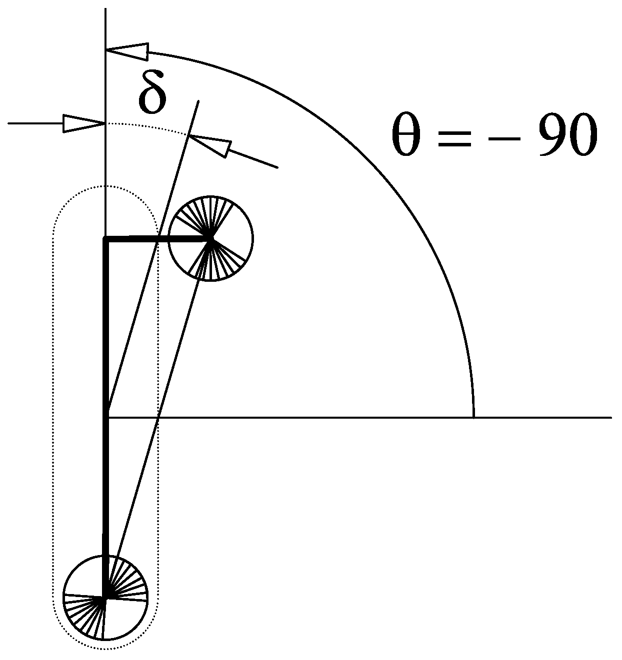Figure 14 depicts how the singularity expected when $\theta =-{90}^{\circ }$ is avoided because of the aforementioned displacement of $m_2$. For the values of our device, $\delta =0.{682}^{\circ }$.

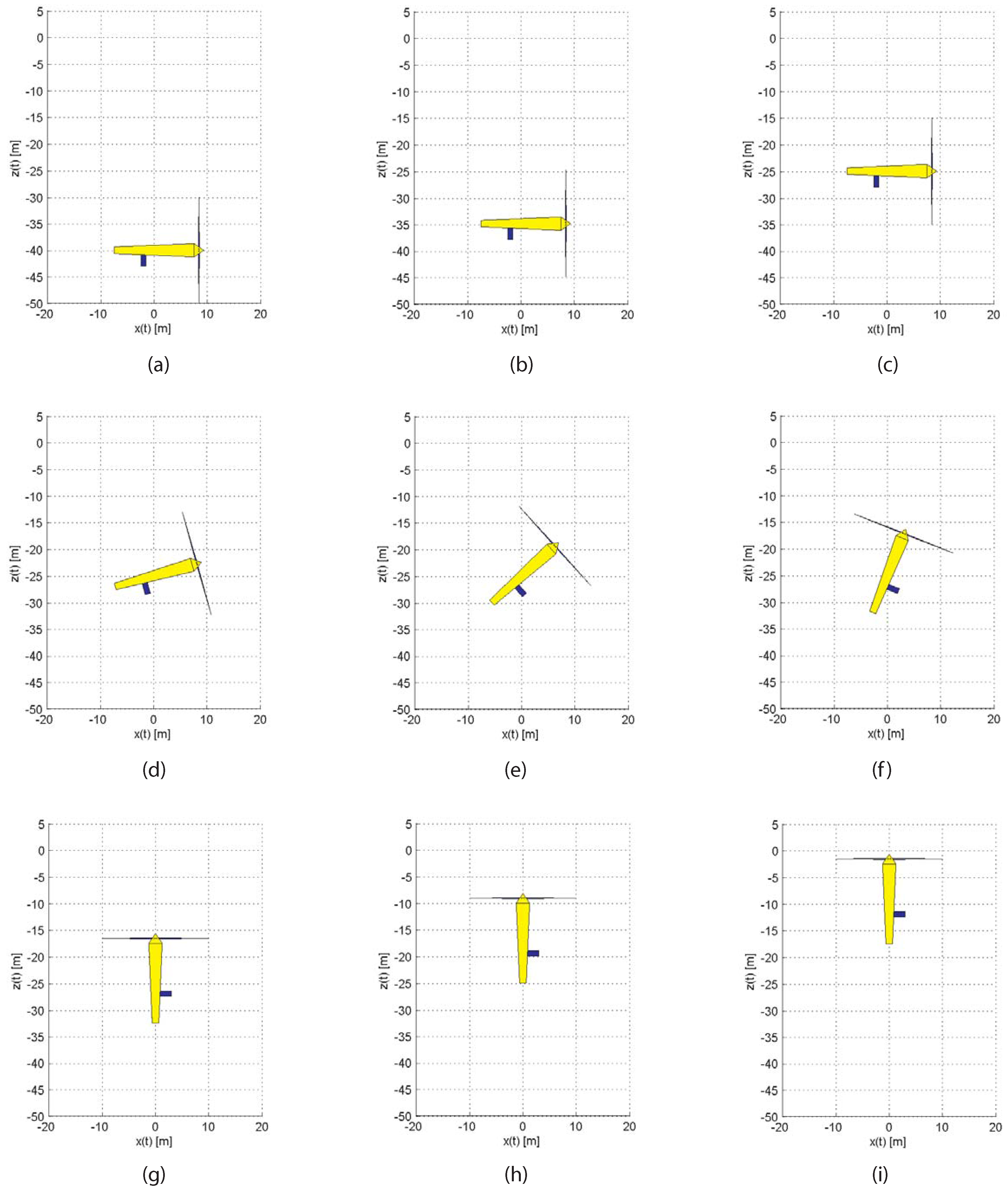
Finally, a visual snapshot of the sequence performed is illustrated in Figure 15, showing the changes in depth and orientation of the device throughout the entire maneuver.

5. Conclusions

The exploitation of renewable energy from tides and ocean currents when the water column is less than 40 m allows the installation of the so-called first generation devices. New solutions to the automation of TEC emersion/immersion maneuvers are therefore being sought in order to improve their economic competitiveness. Periodic maintenance reviews are necessary, during which the device has to be removed from its base and extracted to the surface of the sea. After an appropriate review and carrying out the appropriate maintenance tasks, the power unit must then be returned to the same place on the base. The automation of emersion/immersion maneuvers should therefore be considered. The performance of these automated maneuvers is based on the correct closed loop control of the ballast water that is located inside the nacelle of the main power unit and is used as an actuator to produce vertical forces. Some aspects of the nacelle have therefore been redesigned in order to include ballast tanks and the correct location of the equipment inside in order to permit the depth and the orientation of the device to be controlled by handling ballast water and producing adequate vertical forces obtained from a closed loop control system.

This paper proposes a very simple dynamic model that can be used to control a first generation TEC that was conceived of to harness energy from marine currents. The dynamic model is provided by two degrees of freedom and is composed of only two lumped masses placed on a plane. The control of these two degrees of freedom is performed solely by the ballast water that is located inside the nacelle of the main power unit and is used as an actuator to produce buoying vertical forces (conceived of as volume-increasing devices). A nonlinear control law based on friction compensation for the closed loop depth and/or orientation control is also proposed in order to ensure an adequate behavior when the TEC performs emersion and immersion maneuvers with only passive buoyancy forces. The control scheme is composed of an inner loop based on the dynamic model of the first generation TEC formed of a linear and decoupled input/output relationship and the vector of friction and compressibility terms and an outer loop based on a stabilizing linear control action, which operates with the tracking error vector. The proposed control method demonstrates that it is a simple control strategy, which is computationally efficient and easily implementable in a microprocessor-/microcontroller-based system. Finally, numerical simulations are performed in order to verify that the above-designed controller performs very well in terms of generator controllability, ability to perform emersion and immersion maneuvers with only passive buoyancy forces, quick convergence of the tracking errors to a small neighborhood of zero, smooth transient responses, low control effort and robustness in the case of model parametric uncertainties. Various emersion sequences have been designed to illustrate the capability of the TEC to perform different maintenance tasks, such as general maintenance tasks in the nacelle and blade-cleaning maintenance tasks. The results obtained show that the system performs extremely well with the desired settling time and with no overshoot, even when the device is not always fully submerged and when some free-surface interaction occurs. Finally, the generation of different control strategies and new trajectory generations will be the topics of our future research in order to improve the performance of the automated emersion/immersion maneuvers.