Short-Term Price Forecasting Models Based on Artificial Neural Networks for Intraday Sessions in the Iberian Electricity Market

Abstract

This paper presents novel intraday session models for price forecasts (ISMPF models) for hourly price forecasting in the six intraday sessions of the Iberian electricity market (MIBEL) and the analysis of mean absolute percentage errors (MAPEs) obtained with suitable combinations of their input variables in order to find the best ISMPF models. Comparisons of errors from different ISMPF models identified the most important variables for forecasting purposes. Similar analyses were applied to determine the best daily session models for price forecasts (DSMPF models) for the day-ahead price forecasting in the daily session of the MIBEL, considering as input variables extensive hourly time series records of recent prices, power demands and power generations in the previous day, forecasts of demand, wind power generation and weather for the day-ahead, and chronological variables. ISMPF models include the input variables of DSMPF models as well as the daily session prices and prices of preceding intraday sessions. The best ISMPF models achieved lower MAPEs for most of the intraday sessions compared to the error of the best DSMPF model; furthermore, such DSMPF error was very close to the lowest limit error for the daily session. The best ISMPF models can be useful for MIBEL agents of the electricity intraday market and the electric energy industry.

1. Introduction

The Iberian electricity market (MIBEL) was created in 2004 as a joint initiative from the governments of Portugal and Spain, involving the integration of their respective electric power systems and their previous electricity markets. The MIBEL allows any consumer in the Iberian region (mainland of Portugal and Spain) to purchase electrical energy under a free competition regime from any producer or retailer acting in that region. It represents a regional electricity market with a remarkable growth of renewable energy production that frequently pushes the most expensive thermal power stations outside the generation scheduling of the wholesale market [1]. The MIBEL consists of the forward markets, managed by the company Iberian Energy Market Operator–Portuguese Division (OMIP) [2], and the daily and intraday markets, both managed by the company Iberian Energy Market Operator–Spanish Division (OMIE) [3]. The daily and intraday markets are organized in a daily session, where next-day sale and electricity purchase transactions are carried out, and in six intraday sessions that consider energy offer and demand, which may arise in the hours following the daily viability schedule fixed after the daily session.

Short-term electricity price forecasting (STEPF) has attracted the attention of many researchers in the last years. The previous knowledge on the forecasted hourly prices that will be settled in the pool constitutes very valuable information for any agent involved in the electricity markets. A considerable amount of research has been dedicated to bidding procedures, trading strategies or electricity market offerings—especially for wind farms [4,5,6], price-makers [7,8], and wind farms enhanced with storage capability [9]—and even for bidding in micro grids with renewable generation [10]. Consequently, accurate price forecasts are of significant interest for electric power plants. Thus, according to pool price forecasts, mainly electric energy producers and also distribution utilities and large customers from the demand-side, can change their bidding policy in order to obtain the maximum profit. However, pool prices are hard to forecast due to some characteristics such as non-stationary mean and variance, multiple seasonality, calendar effect, high volatility and high percentage of outliers [11].

Additionally, the price forecasting can also influence the consumers’ demand response [12,13,14]. On the one hand, effective demand response is related to demand forecasting (as well as renewable power forecasting) and, on the other hand, it is associated with price forecasting for the consumers as well as price forecasting of the pool market. Such demand response has to consider interactions among prices, consumer demands and renewable power generation. Research works are starting to develop advanced STEPF models and several other short-term forecasting models for other technical magnitudes, in diverse spatio-temporal scales, in order to support complex systems for research on demand response [15,16,17]. In this sense, suitable STEPF models for intraday sessions are expected that also will play a key role in related research developments.

The immediate application of STEPF models in bidding strategies has propelled the development of this kind of forecasting model. Most of the STEPF models reported are focused on the application to the daily market. The techniques used include those of traditional time series such as auto-regressive integrated moving average (ARIMA) [18,19,20,21] or other artificial intelligence-based techniques such as artificial neural networks (ANNs) [19,22,23,24,25] and fuzzy inference systems (FIS) [26]. Some authors propose hybrid approaches combining two or more techniques in the forecasting model [27,28,29,30,31,32]. In general, most of the published articles are focused on the description of the forecasting techniques and its application to the daily market. The analysis of the price explanatory variables used to build STEPF models is barely studied [33], although this analysis has been pointed out as the focus on STEPF models for the next years [34].

Only a few published works deal with the development of STEPF models in applications to the intraday prices of an electricity market [35,36], although intraday prices are of prime importance in day-to-day market operations, in particular for applications in trading of power plant productions [37,38], or for applications in implementing effective demand response as mentioned above [12,13,14,15,16,17,39]. In [35], a strategic energy bidding for a wind power farm is presented including a very brief description of a STEPF model used for intraday session prices forecasting based on classic time series, but their performance in each of the six sessions of the MIBEL is not indicated. Another research work [36] is focused on maximizing the profit of a wind power producer placed in Holland by using day-ahead and cross-border intraday markets; it seems to utilize a classic seasonal autoregressive integrated moving average (SARIMA) modeling, which is not described, for one-month price forecasts in the intraday German market. The hourly prices settled in intraday sessions in the MIBEL have been studied [40,41]. Their correlations [40] or realized volatility [41] have been highlighted, but no STEPF model for intraday session prices in the MIBEL has been presented in scientific literature describing the best selection of input variables among an extensive set of intraday price explanatory variables, by obtaining mean absolute percentage errors (MAPEs) of forecasts for each of the six intraday session prices and also by comparing them with respect to error of the day-ahead price forecast in the MIBEL.

In general, as indicated above, most of the published papers described the forecasting technique: there are advanced versatile techniques with similar accuracy when they are applied to a specific STEPF case using the same variables and time period. Sometimes authors compare the results obtained with their models with respect to those reported in other works, using the same data and the same period. This paper is not concentrated on forecasting techniques, but it deals with the “forecasting modelling”, that is, on the analysis of extensive sets of explanatory variables and their influence in price forecasts. Furthermore, the forecasting modelling of this paper permits to determine input data and structures of processing appropriate for application to the MIBEL.

This paper presents novel STEPF models developed to be applied to the six intraday sessions of the MIBEL, which are called intraday session models for price forecasts (ISMPF model). The best ISMPF model for each session is described in the paper as well as the selected combination of their input variables. The paper also analyses the forecasting errors achieved using different combinations of input (price explanatory) variables in order to determine the best model which uses the proper combination.

The process for analyzing combinations of explanatory variables is initially used for daily session models for price forecasts (DSMPF models) and for reference models for price estimation (RMPE models) in the daily session of the MIBEL. This process is applied to ISMPF models afterwards in the intraday sessions of the MIBEL. The main characteristics of these models are described in the following paragraphs:

• DSMPF models, developed for the day-ahead hourly price forecasting in the daily session of the MIBEL, consider an extensive set of explanatory variables which include recent prices, regional aggregation of power demands and power generations, hourly time series records of power demand forecasts, wind power generation forecasts and weather forecasts as well as chronological information.
• RMPE models, developed for the estimation of the hourly prices in the daily session, use actual power generations and actual power demands of the day-ahead instead of these variables in the previous day, and the same forecast variables, price variables and chronological information of DSMPF models. They allow the calculation of the lowest limit of error values achievable with the utilized explanatory variables.
• ISMPF models, developed for the hourly price forecasting in the six intraday sessions of the MIBEL, consider the input variables included in DSMPF models as well as the hourly prices of the daily session and hourly prices of previous intraday sessions.

The MIBEL was used to test the models of this paper. On one hand, the best ISMPF models achieved very satisfactory MAPEs for the intraday sessions of the MIBEL, which were lower errors for most of the intraday sessions than the error of the best DSMPF model. On the other hand, the MAPE of the best DSMPF model was very close to the lowest limit error of the best RPME model for the daily session. The best ISMPF model, its performance in the MIBEL and its input variables can constitute valuable information for MIBEL agents of the electricity intraday market and the electric energy industry.

The structure of this paper is the following: Section 2 contains a description of time frameworks for the forecasting models and reference models as well as the characteristics of data corresponding to the MIBEL for hourly price forecast purposes; Section 3 describes RMPE models (reference models) for the hourly prices estimation; Section 4 presents DSMPF models for day-ahead hourly price forecasts; Section 5 describes ISMPF models for hourly price forecasts of the six intraday sessions of the MIBEL; lastly, the conclusions of this paper are presented in Section 6.

2. Time Frameworks and Data Characteristics for Forecasting Models and Reference Models

Time frameworks for day-ahead and intraday MIBEL price forecasting models as well as for reference models are described in Section 2.1. Afterwards, Section 2.2 shows data characteristics corresponding to the MIBEL for the hourly price forecasting.

2.1. Time Frameworks

The description of time frameworks corresponding to DSMPF models and reference models is presented in Section 2.1.1; Section 2.1.2 describes a time framework for ISMPF models.

2.1.1. Time Frameworks for Daily Session Models for Price Forecasts and Reference Models

Bidding offers to the day-head electricity market and the implementation of other power system operation functions are mainly prepared based on short-term forecasting models that provide forecasted hourly prices of the day-ahead.

DSMPF models use as input variables (price explanatory variables) recorded time series of hourly prices in previous days, regional-aggregated hourly power demands and hourly power generations of most of the types of electricity production in the previous day, forecasts of demand, wind power generation and weather (hourly wind speed, temperature and irradiation) for the day-ahead in the region, and chronological variables.

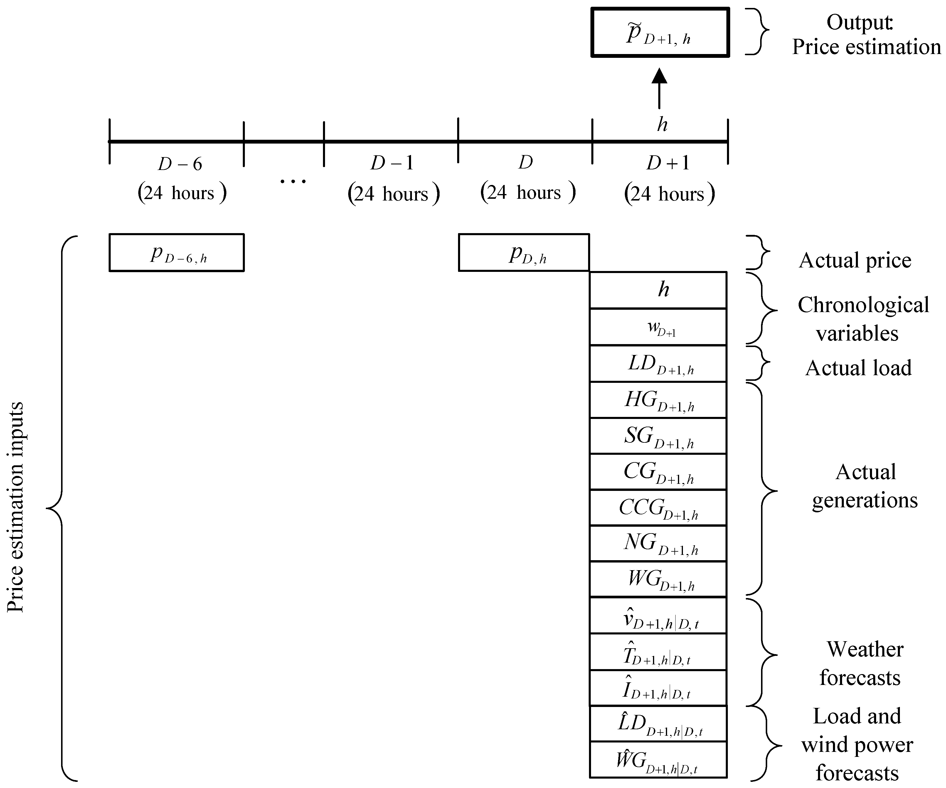
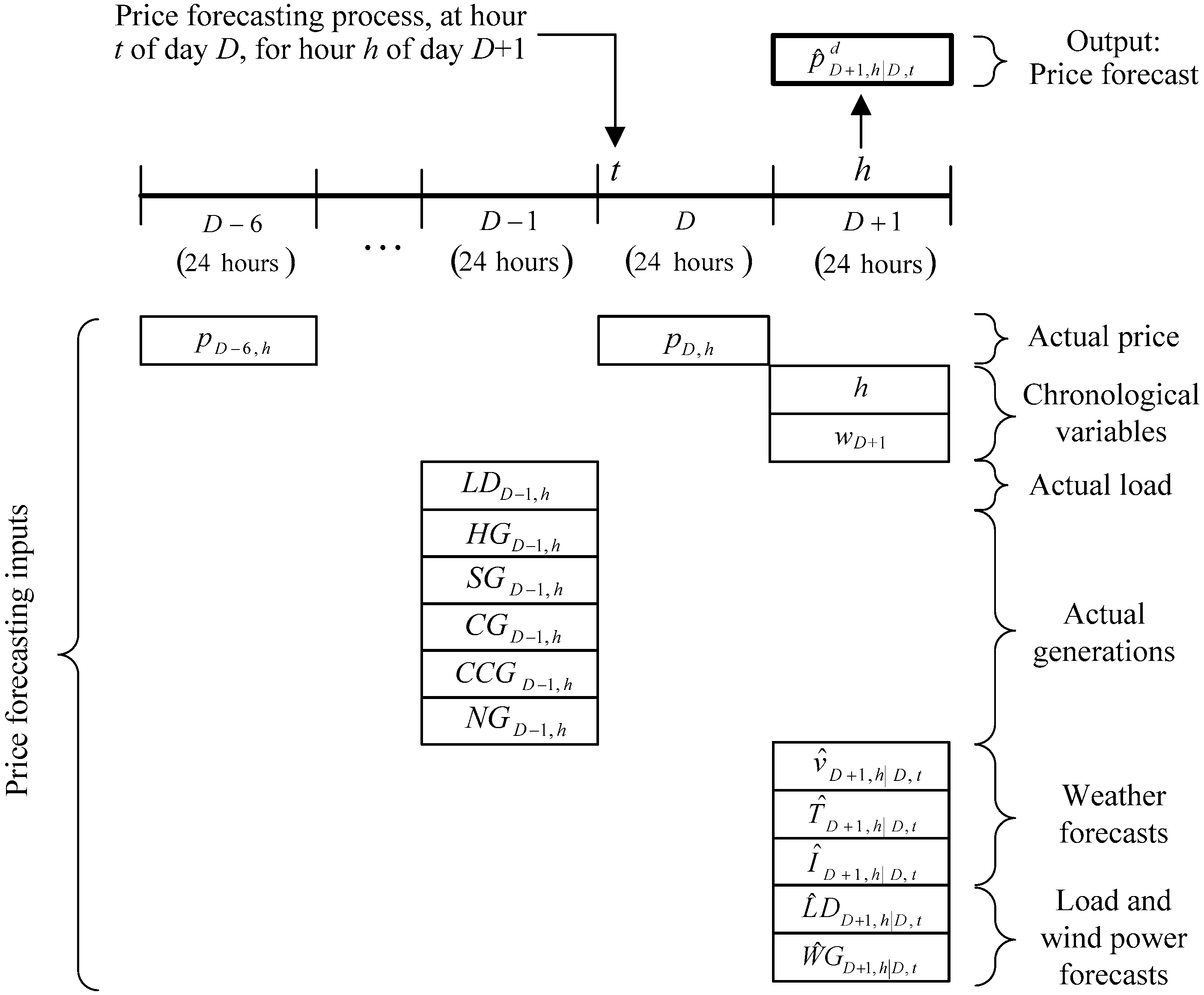
The time framework of DSMPF models is shown in Figure 1. The price forecast ${\widehat{p}}_{D+1,\hspace{0.17em}h|D,\hspace{0.17em}t}^d$ is obtained at hour t of the day D for each hour h of the 24 h in day D + 1. The delivery of the price forecast is assumed in hour t of day D which can be any instant prior to the opening of the daily market session and after the moment in which the forecasted variables corresponding to demand and wind power generation for the day D + 1 are known.

The price for hour h of the day D, $p_{D,h}$, and the price $p_{D-6,h}$ for hour h of day D − 6, are inputs to forecast the price for the hour h of day D + 1. Other inputs are the week day $w_{D+1}$ and hour h of day D + 1, and the weather forecasts obtained at the first hours of day D for the geographical region corresponding to the electricity market and for hour h of day D + 1, that is, the regional weighted forecasted hourly wind speeds ${\widehat{v}}_{D+1,h|D,t}$, regional weighted forecasted hourly temperatures ${\widehat{T}}_{D+1,h|D,t}$ and regional weighted forecasted hourly irradiations ${\widehat{I}}_{D+1,h|D,t}$. These last inputs are similar to those used by authors in [33].

Diverse input variables were included in Figure 1: power demand LD_D−1,h, hydropower generation HG_D−1,h, solar power generation and power cogeneration SG_D−1,h, coal power generation CG_D−1,h, combined cycle power generation CCG_D−1,h, and nuclear power generation NG_D−1,h at hour h of day D − 1. Two additional input variables of forecasting available before the opening of the daily session in day D were considered: power demand forecast $\widehat{L}{D}_{D+1,h|D,t}$ and wind power generation forecast $\widehat{W}{G}_{D+1,\hspace{0.17em}h|D,\hspace{0.17em}t}$ for hour h of day D + 1.

Figure 2 illustrates the time framework of the RMPE models. A part of the input variables of the RMPE models, mainly actual power generations and power demands of day D + 1, as well as the output variable price estimation ${\tilde{p}}_{D+1,\hspace{0.17em}h}$, are different from the input variables of DSMPF models. Note that DSMPF models mainly use actual power generations and power demands of day D − 1 as input variables, and the output variable corresponds to the price forecast ${\widehat{p}}_{D+1,\hspace{0.17em}h|D,\hspace{0.17em}t}^d$. Thus, RMPE models are not forecasting models, but models for hourly price estimation.

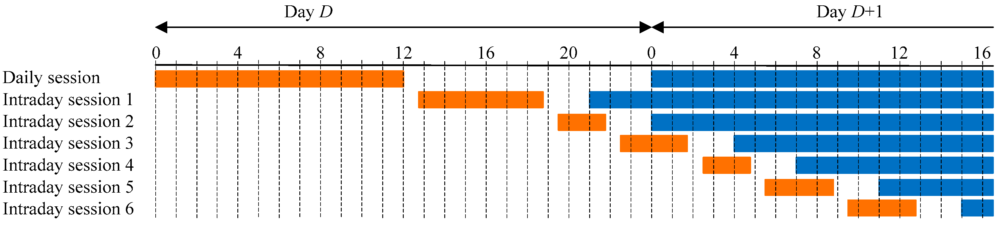
2.1.2. Time Framework of Intraday Session Models for Price Forecasts

The MIBEL market is organized in a daily session whose closing time takes place at 12:00 a.m. (Spanish official hour) of day D and six intraday sessions whose structure is given in

Table 1. Structure of the Iberian electricity market’s (MIBEL’s) intraday sessions.

Session Number	Session Opening Hour (Spanish Hour)	Session Closing Hour (Spanish Hour)	Time Period	Hours in Time Period
1	17:00	18:45	21 (D)–23 (D + 1)	27
2	21:00	21:45	00 (D + 1)–23 (D + 1)	24
3	01:00	01:45	04 (D + 1)–23 (D + 1)	20
4	04:00	04:45	07 (D + 1)–23 (D + 1)	17
5	08:00	08:45	11 (D + 1)–23 (D + 1)	13
6	12:00	12:45	15 (D + 1)–23 (D + 1)	9

. As it is shown, the first intraday session covers the last 3 h of the current day (D) and the 24 h of the following day (D + 1), that is, a total of 27 h. The other sessions comprise only a shorter time period of day D + 1. The time period covered by each session is reduced session after session with a minimum of 9 h in the sixth intraday session.

The time framework for the ISMPF models is illustrated in Figure 3. The input variables of these ISMPF models for a given intraday session can include the hourly prices of previous intraday sessions and the hourly prices of the daily session of the MIBEL, as well as the set of input variables used by DSMPF models. Figure 3 shows in orange the periods in which the forecast can be carried out, from the moment when the prices of the previous session are known (around 45 min after its closing hour) to the closing hour of the corresponding intraday session. Figure 3 also partially shows in blue the period covered by each market session.

2.2. Data Characteristics

For the development of the proposed hourly price forecasting models different kinds of variables have been considered, which are the following:

• Actual hourly data prices for the day-ahead and intraday markets available from the market operator OMIE [3].
• Actual hourly data of the power system: load demand, wind power generation, hydropower generation, cogeneration and solar power generation, nuclear power generation, coal power generation, combined cycle power generation and power exchanged with France. These data were obtained by aggregating a very large amount of information from the websites of Redes Energéticas Nacionais (REN), the Portuguese transmission system operator (TSO) [42] and Red Eléctrica de España (REE), the Spanish TSO [43].
• Hourly weather forecasts: weighted average wind speed, solar irradiance and temperature. These forecasted values were obtained with the numerical weather prediction (NWP) mesoscale model WRF NMM [44], initialized with the forecasts provided by the global NWP model GFS [45].
• Hourly variable forecasts of the power system: power demand forecasts and wind power generation forecasts. These forecasts were obtained by aggregating forecast information from the mentioned TSOs.
• Chronological variables (hour, week day).

The data recorded, corresponding to years 2012 and 2013, were divided into an in-sample data set used for training and an out-sample data set used for testing DSMPF, RMPE and ISMPF models. The out-sample data set was composed of complete weeks extracted along the two years of data in order to have a good representation of the different price behaviours along the year. The in-sample and out-sample data sets were defined as follows:

• In-sample data set: all the hours of the days in 2012 and 2013, except those included in the out-sample data set, totalizing 14,184 cases (h).
• Out-sample data set: all the hours of the weeks with numbers 5, 10, 15, 20, 25, 30, 35, 40, 45, 50 in 2012, and weeks number 2, 7, 12, 17, 22, 27, 32, 37, 42, 47 in 2013; a total of 3360 cases (h).

The descriptive statistics of the price variable of the data sets used for each forecasting model are shown in

Table 2. Descriptive statistics of price data.

Dataset	Statistic	Daily	Intraday 1	Intraday 2	Intraday 3	Intraday 4	Intraday 5	Intraday 6
IN-SAMPLE	Mean (€/MWh)	45.02	44.73	44.75	45.69	47.30	48.08	47.90
	Standard Deviation (€/MWh)	16.44	16.19	16.54	16.82	16.60	17.08	18.11
	Maximum (€/MWh)	110.00	132.22	180.30	180.30	131.57	180.30	180.30
	Count (h)	14,184	14,184	14,184	11,820	10,047	7683	5319
OUT-SAMPLE	Mean (€/MWh)	45.88	45.80	46.93	46.91	48.48	49.10	49.03
	Standard Deviation (€/MWh)	15.37	14.69	14.03	14.59	14.37	14.94	16.54
	Maximum (€/MWh)	86.01	129.65	180.30	119.25	129.87	137.23	148.20
	Count (h)	3360	3360	3360	2800	2380	1820	1260

, including their mean value, standard deviation, maximum values (minimum values are 0), and the total of cases (count of hours). For the total cases of intraday session 1, we have only considered the 24 h of the following day instead of the 27 h covered by this session.

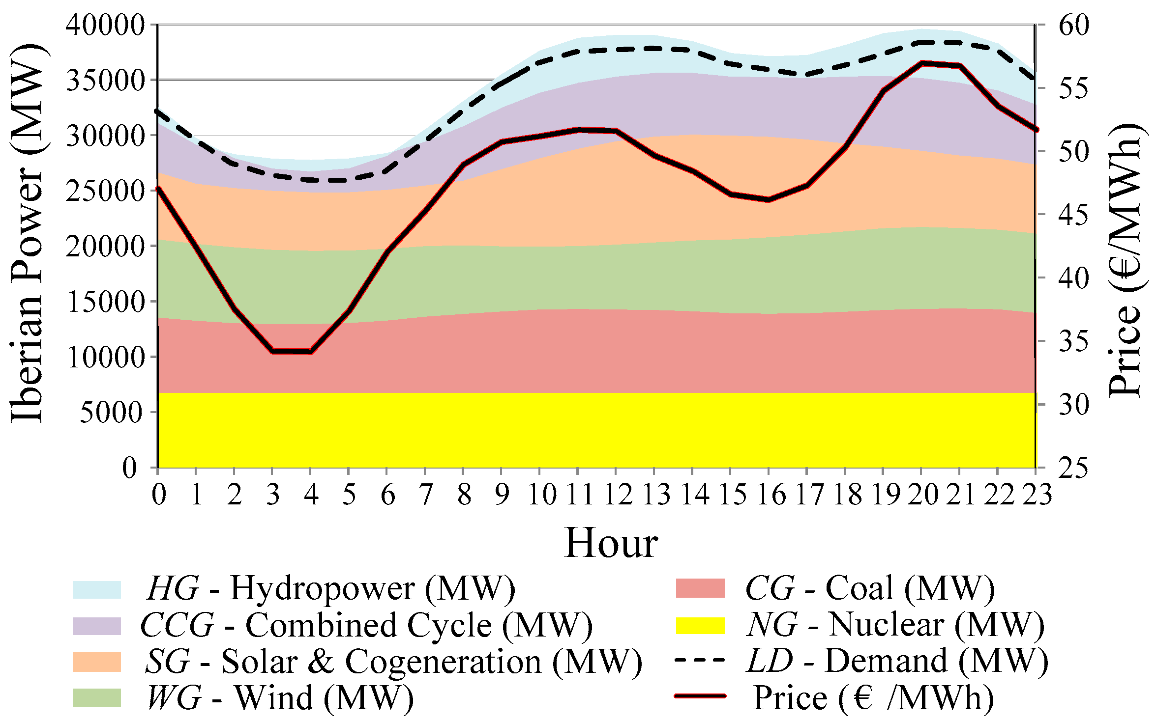
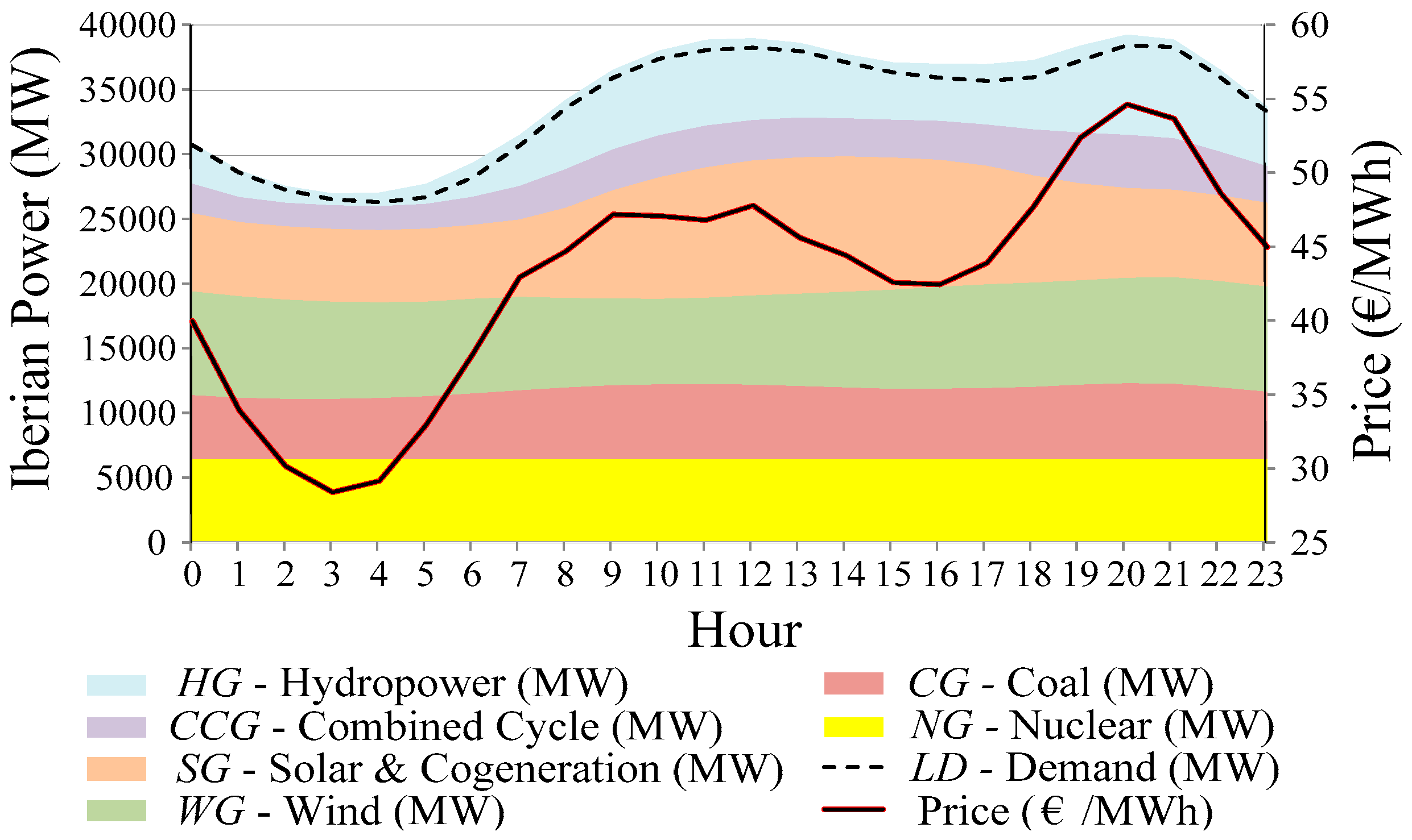
Figure 4 and Figure 5, for years 2012 and 2013 respectively, represent the hourly average values of power generation for each power generation type, power demand and price in the MIBEL. The hourly average power demand was quite similar in these years, although there were slight changes in the generation-mix production. In 2013, the renewable power generation (hydro, solar and wind power productions) was higher than in year 2012. For thermal power generation (combined cycles, coal and nuclear power productions), the electricity generation from nuclear power production was almost the same in both years, but there was a reduction in the other two productions, with a more significant reduction in the combined cycles, caused by a difference between coal and natural gas prices favourable to coal prices in 2013. In 2013, mainly due to a higher renewable proportion of power generation, prices decreased an average of around 4.4 €/MWh.

3. Reference Models for Price Estimation

RMPE models are hourly price estimation models that utilize the variables shown in

Table 3. Variables of reference models for price estimation (RMPE models).

Variable	Description	Range
V1	Hour	0–23
V2	Week day	0 (Monday)–7(special day)
V3	Hourly price D	0–110 €/MWh
V4	Hourly price D − 6	0–110 €/MWh
V5R	Hourly power demand D + 1	20,338–52,853 MW
V6R	Forecasted hourly power demand D + 1	18,200–51,839 MW
V7R	Hourly wind power generation D + 1	161–20,198 MW
V8R	Forecasted hourly wind power generation D + 1	427–19,688 MW
V9R	Forecasted hourly temperature D + 1	−0.8–35.8 °C
V10R	Forecasted hourly wind speed D + 1	1.48–11.15 m/s
V11R	Forecasted hourly irradiance D + 1	0–1031.8 W/m2
V12R	Hourly hydropower generation D + 1	−3957–15,384 MW
V13R	Hourly cogeneration and solar power generation D + 1	3824–13,668 MW
V14R	Hourly coal power generation D + 1	615–11,604 MW
V15R	Hourly nuclear power generation D + 1	3391–7525 MW
V16R	Hourly combined cycled power generation D + 1	336–15,172 MW

as inputs. These input variables include the chronological variables “hour” and “week day” (variables V1 and V2), the prices on previous days at the same hour h (variables V3 and V4), the actual power demand (load) and forecasted power demand variables of the power system for hour h of day D + 1 (variables V5R and V6R), the actual and forecasted wind power generation variables for hour h of day D + 1 (variables V7R and V8R), the weather forecasts of wind speed, temperature and irradiance for hour h of day D + 1 (variables V9R to V11R) and the actual power generations corresponding to hour h of day D + 1 (variables V12R to V16R).

We did not explore the relative importance of the different price explanatory variables considered in this paper since it was extensively presented in a previous publication [33]. Instead, in the present article, a set of studies of suitable combinations of input variables for the different type of models (DSMPF, RMPE and ISMPF models) are being described in order to determine the best DSMPF model, the best RMPE model and the best ISMPF model for each intraday session in the MIBEL.

RMPE models contain the variables of the REMPE model introduced by the authors in [33], but now two additional variables are considered: the forecasted hourly power demand for day D + 1 (variable V6R) and the forecasted hourly wind power generation for day D + 1 (variable V8R). Then, we formulated the question: “How relevant are these forecasted variables (V6R and V8R) compared to the variables of the actual demand D + 1 and the actual wind generation D + 1 (V5R and V7R)?”. In order to answer this question, four RMPE models (model REF1 to model REF4) were built, shown in

Table 4. RMPE models and their mean absolute percentage errors (MAPEs).

Explanatory Variables		Description	REF1	REF2	REF3	REF4
Chronological	V1	Hour (0–23 h)	●	●	●	●
	V2	Week day (1–7)	●	●	●	●
Price	V3	Hourly price (D)	●	●	●	●
	V4	Hourly price (D − 6)	●	●	●	●
Demand	V5R	Hourly power demand D + 1	●	-	●	●
	V6R	Forecasted hourly power demand D + 1	-	●	-	●
Wind PG	V7R	Hourly wind power generation D + 1	●	●	-	●
	V8R	Forecasted hourly wind power generation D + 1	-	-	●	●
Weather	V9R	Forecasted hourly temperature D + 1	●	●	●	●
	V10R	Forecasted hourly wind speed D + 1	●	●	●	●
	V11R	Forecasted hourly irradiance D + 1	●	●	●	●
Other PG	V12R	Hourly hydropower generation D + 1	●	●	●	●
	V13R	Hourly cogeneration and solar power generation D + 1	●	●	●	●
	V14R	Hourly coal power generation D + 1	●	●	●	●
	V15R	Hourly nuclear power generation D + 1	●	●	●	●
	V16R	Hourly combined cycled power generation D + 1	●	●	●	●
MAPE (%)			10.23	9.89	10.43	9.88

. In this table, PG means power generation. Please observe that model REF1 is the REMPE model.

RMPE models were implemented with a multilayer perceptron neural network (MLP) [46], using one hidden layer with 2n + 1 neurons, where n is the number of input variables (explanatory variables). These models were trained and tested with the in-sample and out-sample data sets previously described in Section 2, which were utilized in all computing experiences presented in this paper. Since we used random weight initiation in these neural networks, different training of the same MLP resulted in slightly different computer results (outputs). In order to avoid this inconvenience, we used, as a final forecasting result, the ensemble averaging [47] of the outputs of 20 training processes of the same MLP, thus achieving a more stable response and a lower error.

An error analysis for RMPE models using the MAPE was carried out in the price estimations corresponding to the out-sample data set, where the MAPE is defined by Equation (1):

$$\mathit{MAPE}=\frac{1}{N}{\displaystyle \sum _{T=1}^N\frac{\left|P_{\mathrm{real}\_T}-P_{\mathrm{estimation}\_T}\right|}{P_{\mathrm{real}\_\mathrm{M}}}\hspace{0.17em}100}$$

(1)

where P_{real_T} is the real hourly price value, P_{estimation_T} is the estimation of the hourly price value obtained from each RMPE model, N is the number of elements of the out-sample data set and P_{real_M} is the mean real hourly price value corresponding to that data set.

Variable V6R (forecasted power demand) is used in model REF2 instead of variable V5R (actual power demand) of model REF1. Thus, the MAPEs of Table 4 indicate that the forecasted power demand (for day D + 1) explains electricity prices better than the actual power demand (of day D + 1).

We repeated the experience using variable V8R (forecasted wind power generation) in model REF3 instead of variable V7R (actual wind power generation) in model REF1. Then, the MAPEs of Table 4 indicate that the actual wind power generation (of day D + 1) explains electricity prices better than the forecasted wind power generation (of day D + 1). Furthermore, model REF4 including all variables leads to a MAPE value almost equal to that of model REF2.

Therefore, RMPE models can achieve the best MAPE value of approximately 9.9%. It represents the lowest error (“minimum error”) using the considered explanatory variables, that is, the lowest limit of the possible performance of any model for price estimation or for price forecast belonging to the same class of models with a similar kind of variables to those used in RMPE models.

4. Daily Session Models for Price Forecasts

The inputs of DSMPF models are:

• Chronological variables (“hour” and “week day”);
• Hourly prices of days D and D − 6;
• Recorded hourly power demand and hourly power generations of days D − 1;
• Hourly power demand forecasts and hourly wind power generation forecast for day D + 1; and
• Hourly weather forecasts of wind speed, temperature and irradiance for day D + 1.

Then, DSMPF models take into consideration the sets of input variables shown in

Table 5. Variables of daily session models for price forecasts (DSMPF models).

Variable	Description	Range
V1	Hour	0–23
V2	Week day	0 (Monday)–7 (special day)
V3	Hourly price D	0–110 €/MWh
V4	Hourly price D − 6	0–110 €/MWh
V5	Hourly power demand D − 1	20,338–52,853 MW
V6	Forecasted hourly power demand D + 1	18,200–51,839 MW
V7	Forecasted hourly temperature D + 1	−0.8–35.8 °C
V8	Forecasted hourly wind speed D + 1	1.48–11.15 m/s
V9	Forecasted hourly irradiance D + 1	0–1031.8 W/m2
V10	Forecasted hourly wind power generation D + 1	427–19,688 MW
V11	Hourly hydropower generation D − 1	−3957–15,384 MW
V12	Hourly cogeneration and solar power generation D − 1	3824–13,668 MW
V13	Hourly coal power generation D − 1	615–11,604 MW
V14	Hourly nuclear power generation D − 1	3391–7525 MW
V15	Hourly combined cycled power generation D − 1	336–15,172 MW

. Obviously, variables of DSMPF models V6, V7, V8, V9 and V10 correspond to variables V6R, V9R, V10R, V11R and V8R used in RMPE models (Table 3).

DSMPF models were implemented with MLPs with the same structure used for the RMPE models, that is, one hidden layer with 2n + 1 neurons, where n is the number of input explanatory variables. For the training and testing of the MLP, in-sample and out-sample data sets previously described in Section 2 were used again, as well as the abovementioned ensemble technique for the corresponding computer results.

In a similar way than that followed for RMPE models, the MAPE was calculated for the price forecasts corresponding to the out-sample data set for DSMPF models. In this case, the MAPE is defined by Equation (2):

$$\mathit{MAPE}=\frac{1}{N}{\displaystyle \sum _{T=1}^N\frac{\left|P_{\mathrm{real}\_T}-P_{\mathrm{forecast}\_T}\right|}{P_{\mathrm{real}\_\mathrm{M}}}\hspace{0.17em}100}$$

(2)

where P_{real_T} is the real hourly price value, P_{forecast_T} is the forecasted hourly price value of the forecasting model, N is the number of elements in the out-sample data set, and P_{real_M} is the mean real hourly price value corresponding to that data set.

In the following paragraphs, a summary of variable selection studies for DSMPF models is shown corresponding to reasonable combinations of variables (grouped by their common characteristics) in order to look for the best MAPE, that is, the best DSMPF model.

The MAPEs for DSMPF models (M1 to M18), with different input variables, are presented in

Table 6. DSMPF models and their MAPEs.

Explanatory Variables		M1	M2	M3	M4	M5	M6	M7	M8	M9	M10	M11	M12	M13	M14	M15	M16	M17	M18
Chronological	V1	●	●	●	●	●	●	●	●	●	●	●	●	●	●	●	●	●	●
	V2	●	●	●	●	●	●	●	●	●	●	●	●	●	●	●	●	●	●
Price	V3	-	●	●	●	●	●	●	●	●	●	●	●	●	●	●	●	●	●
	V4	-	-	●	●	●	●	●	●	●	●	●	●	●	●	●	●	●	●
Demand	V5	-	-	-	●	●	●	●	●	●	●	●	●	●	●	●	●	●	●
	V6	-	-	-	-	●	●	●	●	●	●	●	●	●	●	●	●	●	●
Weather	V7	-	-	-	-	-	●	-	-	-	-	●	●	●	●	●	●	●	●
	V8	-	-	-	-	-	-	●	-	-	●	-	-	-	-	-	-	-	-
	V9	-						-	●	-	-	-	-	-	-	-	-	-	-
Power generation	V10	-	-	-	-	-	-	-	-	●	●	●	●	●	●	●	●	●	●
	V11	-	-	-	-	-	-	-	-	-	-	-	●		-	-	-	●	●
	V12	-	-	-	-	-	-	-	-	-	-	-	-	●	-	-	-	●	-
	V13	-	-	-	-	-	-	-	-	-	-	-	-	-	●	-	-	-	●
	V14	-	-	-	-	-	-	-	-	-	-	-	-	-	-	●	-	-	●
	V15	-	-	-	-	-	-	-	-	-	-	-	-	-	-	-	●	-	●
MAPE (%)		20.83	17.00	16.81	16.70	16.33	16.37	12.85	16.40	11.64	11.86	11.58	10.86	11.41	11.54	11.43	11.54	11.00	10.69

. The selection of variables follows an ordered analysis, such that only some DSMPF models are presented in the table for conclusive purposes. The construction of Table 6 corresponds to a selection process with the following sequence:

• Models M1 to M3 for price variables selection;
• Models M4 and M5 for selection of power demand and forecasted power demand variables;
• Models M6 to M11 for selection of forecasted weather and wind generation variables; and
• Models M12 to M18 for power generation variables selection.

Model M1 is a simple baseline model with a MAPE value of 20.83%, slightly higher than the double of 9.9% achieved by the best RMPE model. As mentioned in the previous section, 9.9% is the lowest limit error value that RMPE models or DSMPF models could obtain.

If variable V3 (hourly price D) is added to those used by model M1 leading to model M2, then the MAPE decreases to 17%. The inclusion of variable V5 (hourly power demand D − 1) in model M4 slightly reduces the MAPE to 16.70%. Additionally, if variable V6 (hourly forecasted power demand D + 1) is included (model M5), the MAPE is reduced to 16.33%.

Models M6–M9, compared to model M5, show an added price explicability by including variables V7–V10 (forecasted weather variables and forecasted wind power generation variable). The forecasted wind power generation variable (V10) in model M9 provides a better performance (MAPE of 11.64%). Alternatively, the forecasted wind speed variable (V8) in model M7 obtains a MAPE of 12.85%.

The two variables V8 and V10 have collinear information, leading to an error of 11.86% (in model M11), which is worse than error 11.64% considering only variable V10 in model M9. However, the use of variable V10 together with variable V7 (forecasted temperature D + 1) improves the performance to a better MAPE value (11.58%) in model M11.

Models M12 to M16 allow the evaluation of the improvement in the MAPE by adding variables V11 to V15 (power generation variables D − 1). Variable V11 (hydropower generation D − 1) is the one that achieves a lower error, 10.86% in model M12. The inclusion of variables V13 to V15 (thermal power generation D − 1) to the previous model M12 results in the best performance of DSMPF models (model M18), reaching a MAPE value of 10.69%, which is very satisfactory in comparison to the aforementioned lowest limit error value of 9.9% of RMPE models.

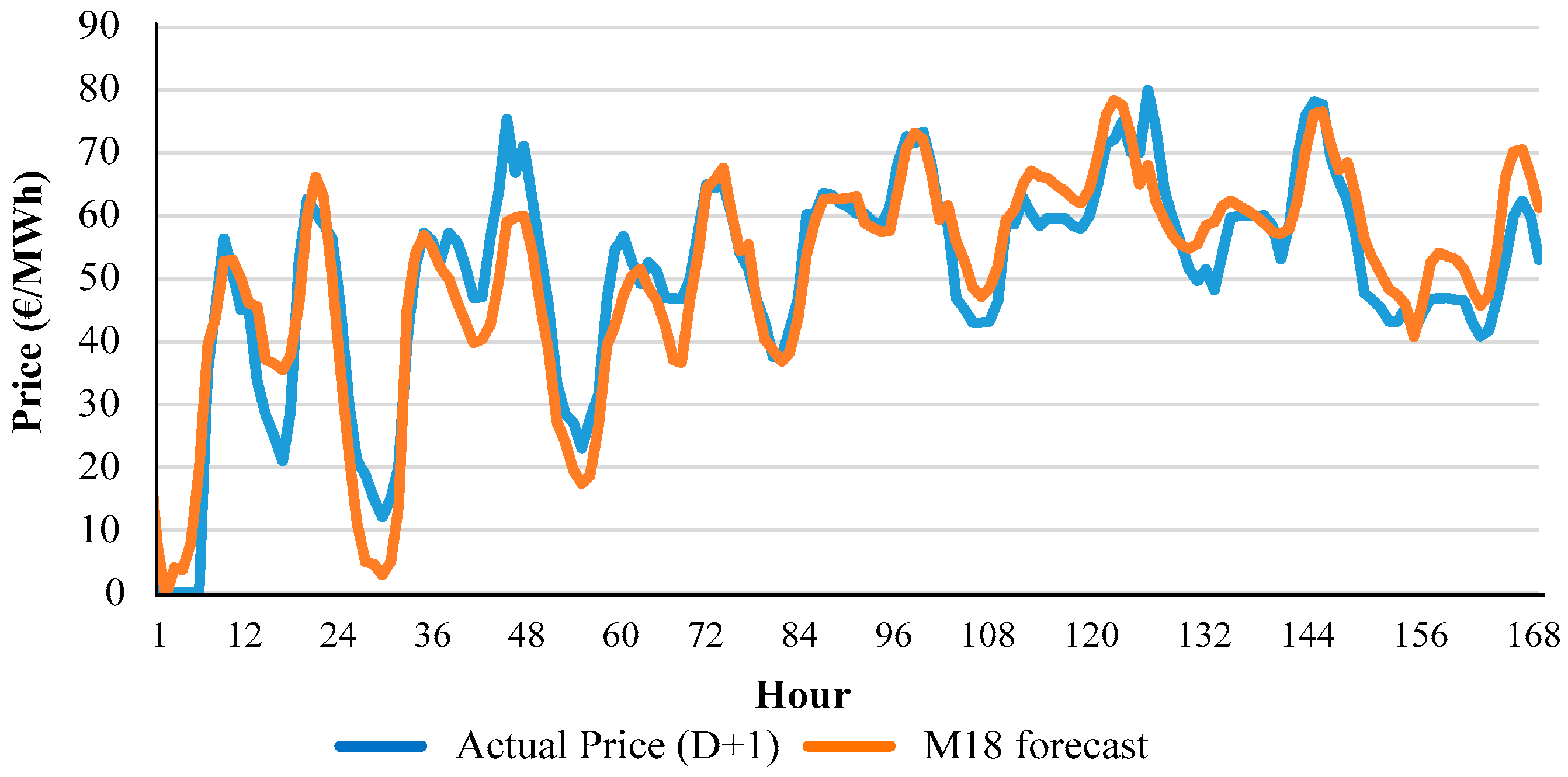
Figure 6 shows an example of the hourly evolution of actual price values and forecasts of model M18 for week 7 of year 2013.

5. Intraday Session Models for Price Forecasts

As indicated in the “Introduction” section, this paper is focused on the ISMPF models corresponding to the six intraday sessions of the MIBEL.

ISMPF models of each intraday session are short-term hourly price forecasting models that can utilize hourly prices on previous days D and D − 6, price values of the daily session and price values of previous intraday sessions of the MIBEL. They also include recorded explanatory variables mainly corresponding to days D − 1 and weather forecasts of day D + 1, as well as power demand forecasts and wind power generation forecasts for day D + 1 in order to forecast the electricity price values of the intraday sessions of the MIBEL.

Thus, six types of explanatory variables were considered in ISMPF models for a given intraday session:

• Chronological variables (“hour” and “week day”);
• Hourly prices of days D and D − 6;
• Hourly prices of the daily session D + 1 and hourly prices of previous intraday sessions of the MIBEL;
• Hourly power demand and hourly power generations of days D − 1;
• Hourly power demand forecasts and hourly wind power generation forecasts for day D + 1;
• Hourly weather forecasts of wind speed, temperature and irradiance for day D + 1.

Then, ISMPF models consider the sets of input variables shown in

Table 7. Variables of ISMPF models.

Variable	Description	Range
V1	Hour	0–23
V2	Week day	0 (Monday)–7 (special day)
V3	Hourly price D	0–110 €/MWh
V4	Hourly price D − 6	0–110 €/MWh
V5I	Hourly price D + 1 of daily session	0–110 €/MWh
V6I	Hourly power demand D − 1	20,338–52,853 MW
V7I	Forecasted hourly power demand D + 1	18,200–51,839 MW
V8I	Forecasted hourly temperature D + 1	−0.8–35.8 °C
V9I	Forecasted hourly wind speed D + 1	1.48–11.15 m/s
V10I	Forecasted hourly irradiance D + 1	0–1031.8 W/m2
V11I	Forecasted hourly wind power generation D + 1	427–19,688 MW
V12I	Hourly hydropower generation D − 1	−3957–15,384 MW
V13I	Hourly cogeneration and solar power generation D − 1	3824–13,668 MW
V14I	Hourly coal power generation D − 1	615–11,604 MW
V15I	Hourly nuclear power generation D − 1	3391–7525 MW
V16I	Hourly combined cycled power generation D − 1	336–15,172 MW
V17I	Hourly price D + 1 from intraday session 1	0–132.22 €/MWh
V18I	Hourly price D + 1 from intraday session 2	0–80.30 €/MWh
V19I	Hourly price D + 1 from intraday session 3	0–180.30 €/MWh
V20I	Hourly price D + 1 from intraday session 4	0–131.57 €/MWh
V21I	Hourly price D + 1 from intraday session 5	0–180.30 €/MWh

. Obviously, variables V6I to V16I of ISMPF models correspond to variables V5 to V15 used in DSMPF models (Table 5).

ISMPF models were implemented with MLPs with the same structure used for DSMPF models, that is, one hidden layer with 2n + 1 neurons, where n is the number of input explanatory variables. For the training and testing of the MLP, in-sample and out-sample data sets previously described in Section 2 were used again as well as the ensemble technique for the corresponding computer results.

In a similar way to that used for DSMPF models, the MAPE was calculated for the price forecasts corresponding to the out-sample data set for DSMPF models. In this case, the MAPE for intraday session k is defined by Equation (3):

$${\mathit{MAPE}}_k=\frac{1}{N_k}{\displaystyle \sum _{T=1}^{N_k}\frac{\left|P_{k \mathrm{real}\_T}-P_{k \mathrm{forecast}\_T}\right|}{{\mathrm{P}}_{\mathrm{real}\_\mathrm{MNk}}}\hspace{0.17em}100}$$

(3)

where P_{kreal_T} is the real hourly price value, P_{kforecast_T} is the forecasted hourly price value of the forecasting model of intraday session k, N_k is the number of elements (h) in the out-sample data set and P_{real_MNk} is the mean real hourly price value corresponding to that data set. The values for N_k were 3360 h for intraday sessions 1 and 2, 2800 h for intraday session 3, 2380 h for intraday session 4, 1820 h for intraday session 5, and 1260 h for intraday session 6.

A summary of variable selection studies of ISMPF models for each intraday session will be presented in Section 5.1, Section 5.2, Section 5.3, Section 5.4, Section 5.5 and Section 5.6, corresponding to reasonable combinations of explanatory variables (grouped by their common characteristics) that allow to achieve the best ISMPF model of such intraday session.

Following a similar process to that used to select suitable variables for DSMPF models (in previous Section 4), a significant number of combinations of variables were analysed for the six intraday sessions, but only ISMPF models that led to relevant conclusions are going to be presented.

The procedure of analysis was based on a sequential integration of a different kind of variables by the following order of importance:

• Chronological variables V1 and V2 (hour and week day);
• Price variables, including price D − 1, price D − 6, price D + 1 of daily session, and price D + 1 of previous intraday sessions;
• Power demand D − 1 and forecasted power demand D + 1;
• Forecasted weather D + 1 and forecasted wind power generation D + 1;
• Power generations D − 1.

An ISMPF model that includes the price D + 1 of the daily session (clearing hourly price for the day ahead D + 1) and the price D + 1 of previous intraday sessions (clearing hourly price D + 1 from previous intraday sessions) can be used immediately after the clearing market for the sessions whose prices are included as inputs in the ISMPF model. Simpler ISMPF models that do not include these variables can be utilized at the first hours of day D in a similar way to DSMPF models presented in Section 4.

Descriptions of ISMPF models for each intraday session are presented in the next paragraphs.

5.1. Intraday Market Session 1

The baseline model S1M1 in

Table 8. ISMPF models for intraday session 1 and their MAPEs.

Explanatory Variables		Description	S1M1	S1M2	S1M3	S1M4	S1M5	S1M6	S1M7	S1M8	S1M9
Chronological	V1	Hour (0–23 h)	●	●	●	●	●	●	●	●	●
	V2	Week day (1–7)	●	●	●	●	●	●	●	●	●
Price	V3	Hourly price (D)	-	●	-	-	●	●	-	-	-
	V4	Hourly price (D − 6)	-	-	●	-	-	●	-	-	-
	V5I	Hourly price (D + 1) from daily session	-	-	-	●	●	●	●	●	●
Demand	V6I	Hourly power demand (D − 1)	-	-	-	-	-	-	●	-	-
	V7I	Forecasted hourly power demand (D + 1)	-	-	-	-	-	-	●	-	-
Weather	V8I	Forecasted hourly temperature (D + 1)	-	-	-	-	-	-	-	●	-
	V9I	Forecasted hourly wind speed (D + 1)	-	-	-	-	-	-	-	●	-
	V10I	Forecasted hourly irradiance (D + 1)	-	-	-	-	-	-	-	●	-
Power generation	V11I	Forecasted hourly wind power generation (D + 1)	-	-	-	-	-	-	-	●	-
	V12I	Hourly hydropower generation (D − 1)	-	-	-	-	-	-	-	-	●
	V13I	Hourly cogeneration and solar power generation (D − 1)	-	-	-	-	-	-	-	-	●
	V14I	Hourly coal power generation (D − 1)	-	-	-	-	-	-	-	-	●
	V15I	Hourly nuclear power generation (D − 1)	-	-	-	-	-	-	-	-	●
	V16I	Hourly combined cycled power generation (D − 1)	-	-	-	-	-	-	-	-	●
MAPE (%)			19.95	16.56	19.64	7.49	7.84	7.51	7.59	7.49	7.48

that uses only chronological information (variables V1 and V2) has a MAPE close to 20%. This order of magnitude of the error was similar for most of the intraday sessions (models S1M1, S2M1, S3M1, S4M1 and S5M1) and it was slightly lower than the error of model M1 (Table 6) for the daily session. Notice that

Table 9. ISMPF models for intraday session 2 and their MAPEs.

Explanatory Variables		Description	S2M1	S2M2	S2M3	S2M4	S2M5	S2M6	S2M7	S2M8	S2M9
Chronological	V1	Hour (0–23 h)	●	●	●	●	●	●	●	●	●
	V2	Week day (1–7)	●	●	●	●	●	●	●	●	●
Price	V3	Hourly price (D)	-	●	-	-	-	-	-	-	-
	V4	Hourly price (D − 6)	-	-	●	-	-	-	-	-	-
	V5I	Hourly price (D + 1) from daily session	-	-	-	●	-	●	●	●	●
	V17I	Hourly price (D + 1) from intraday session 1	-	-	-	-	●	●	●	●	●
Demand	V6I	Hourly power demand (D − 1)	-	-	-	-	-	-	●	-	-
	V7I	Forecasted hourly power demand (D + 1)	-	-	-	-	-	-	●	-	-
Weather	V8I	Forecasted hourly temperature (D + 1)	-	-	-	-	-	-	-	●	-
	V9I	Forecasted hourly wind speed (D + 1)	-	-	-	-	-	-	-	●	-
	V10I	Forecasted hourly irradiance (D + 1)	-	-	-	-	-	-	-	●	-
Power generation	V11I	Forecasted hourly wind power gen. (D + 1)	-	-	-	-	-	-	-	●	-
	V12I	Hourly hydropower generation (D − 1)	-	-	-	-	-	-	-	-	●
	V13I	Hourly cogeneration and solar power generation (D − 1)	-	-	-	-	-	-	-	-	●
	V14I	Hourly coal power generation (D − 1)	-	-	-	-	-	-	-	-	●
	V15I	Hourly nuclear power generation (D − 1)	-	-	-	-	-	-	-	-	●
	V16I	Hourly combined cycled power generation (D − 1)	-	-	-	-	-	-	-	-	●
MAPE (%)			19.84	16.71	19.61	9.84	9.95	8.85	8.90	9.03	9.16

,

Table 10. ISMPF models for intraday session 3 and their MAPEs.

Explanatory Variables		Description	S3M1	S3M2	S3M3	S3M4	S3M5	S3M6	S3M7	S3M8	S3M9	S3M10
Chronological	V1	Hour (0–23 h)	●	●	●	●	●	●	●	●	●	●
	V2	Week day (1–7)	●	●	●	●	●	●	●	●	●	●
Price	V3	Hourly price (D)	-	●	-	-	-	-	-	-	-	-
	V4	Hourly price (D − 6)	-	-	●	-	-	-	-	-	-	-
	V5I	Hourly price (D + 1) from daily session	-	-	-	●	-	-	●	●	●	●
	V17I	Hourly price (D + 1) from intraday session 1	-	-	-	-	●	-	●	●	●	●
	V18I	Hourly price (D + 1) from intraday session 2	-	-	-	-	-	●	●	●	●	●
Demand	V6I	Hourly power demand (D − 1)	-	-	-	-	-	-	-	●	-	-
	V7I	Forecasted hourly power demand (D + 1)	-	-	-	-	-	-	-	●	-	-
Weather	V8I	Forecasted hourly temperature (D + 1)	-	-	-	-	-	-	-	-	●	-
	V9I	Forecasted hourly wind speed (D + 1)	-	-	-	-	-	-	-	-	●	-
	V10I	Forecasted hourly irradiance (D + 1)	-	-	-	-	-	-	-	-	●	-
Power generation	V11I	Forecasted hourly wind power gen. (D + 1)	-	-	-	-	-	-	-	-	●	-
	V12I	Hourly hydropower generation (D − 1)	-	-	-	-	-	-	-	-	-	●
	V13I	Hourly cogeneration and solar power generation (D − 1)	-	-	-	-	-	-	-	-	-	●
	V14I	Hourly coal power generation (D − 1)	-	-	-	-	-	-	-	-	-	●
	V15I	Hourly nuclear power generation (D − 1)	-	-	-	-	-	-	-	-	-	●
	V16I	Hourly combined cycled power generation (D − 1)	-	-	-	-	-	-	-	-	-	●
MAPE (%)			19.96	17.36	19.50	10.98	10.23	9.40	9.30	10.31	9.70	10.09

,

Table 11. ISMPF models for intraday session 4 and their MAPEs.

Explanatory Variables		Description	S4M1	S4M2	S4M3	S4M4	S4M5	S4M6	S4M7	S4M8	S4M9	S4M10	S4M11
Chronological	V1	Hour (0–23 h)	●	●	●	●	●	●	●	●	●	●	●
	V2	Week day (1–7)	●	●	●	●	●	●	●	●	●	●	●
Price	V3	Hourly price (D)	-	●	-	-	-	-	-	-	-	-	-
	V4	Hourly price (D − 6)	-	-	●	-	-	-	-	-	-	-	-
	V5I	Hourly price (D + 1) from daily session	-	-	-	●	-	-	●	●	●	●	●
	V17I	Hourly price (D + 1) from intraday session 1	-	-	-	-	●		●	●	●	●	●
	V18I	Hourly price (D + 1) from intraday session 2	-	-	-	-	-	●	●	●	●	●	●
	V19I	Hourly price (D + 1) from intraday session 3	-	-	-	-	-	-	●	●	●	●	●
Demand	V6I	Hourly power demand (D − 1)	-	-	-	-	-	-	-	-	●	-	-
	V7I	Forecasted hourly power demand (D + 1)	-	-	-	-	-	-	-	-	●	-	-
Weather	V8I	Forecasted hourly temperature (D + 1)	-	-	-	-	-	-	-	-	-	●	-
	V9I	Forecasted hourly wind speed (D + 1)	-	-	-	-	-	-	-	-	-	●	-
	V10I	Forecasted hourly irradiance (D + 1)	-	-	-	-	-	-	-	-	-	●	-
Power generation	V11I	Forecasted hourly wind power generation (D + 1)	-	-	-	-	-	-	-	-	-	●	-
	V12I	Hourly hydropower generation (D − 1)	-	-	-	-	-	-	-	-	-	-	●
	V13I	Hourly cogeneration and solar power generation (D − 1)	-	-	-	-	-	-	-	-	-	-	●
	V14I	Hourly coal power generation (D − 1)	-	-	-	-	-	-	-	-	-	-	●
	V15I	Hourly nuclear power generation (D − 1)	-	-	-	-	-	-	-	-	-	-	●
	V16I	Hourly combined cycled power generation (D − 1)	-	-	-	-	-	-	-	-	-	-	●
MAPE (%)			19.80	16.42	19.08	11.99	10.86	10.60	10.52	9.08	9.31	9.37	9.49

,

Table 12. ISMPF models for intraday session 5 and their MAPEs.

Explanatory Variables		Description	S5M1	S5M2	S5M3	S5M4	S5M5	S5M6	S5M7	S5M8	S5M9	S5M10	S5M11	S5M12
Chronological	V1	Hour (0–23 h)	●	●	●	●	●	●	●	●	●	●	●	●
	V2	Week day (1–7)	●	●	●	●	●	●	●	●	●	●	●	●
Price	V3	Hourly price (D)	-	●	-	-	-	-	-	-	-	-	-	-
	V4	Hourly price (D − 6)	-	-	●	-	-	-	-	-	-	-	-	-
	V5I	Hourly price (D + 1) from daily session	-	-	-	●	-	-	-	-	●	●	●	●
	V17I	Hourly price (D + 1) from intraday session 1	-	-	-	-	●	-	-	-	●	●	●	●
	V18I	Hourly price (D + 1) from intraday session 2	-	-	-	-	-	●	-	-	●	●	●	●
	V19I	Hourly price (D + 1) from intraday session 3	-	-	-	-	-	-	●	-	●	●	●	●
	V20I	Hourly price (D + 1) from intraday session 4	-	-	-	-	-	-	-	●	●	●	●	●
Demand	V6I	Hourly power demand (D − 1)	-	-	-	-	-	-	-	-	-	●	-	-
	V7I	Forecasted hourly power demand (D + 1)	-	-	-	-	-	-	-	-	-	●	-	-
Weather	V8I	Forecasted hourly temperature (D + 1)	-	-	-	-	-	-	-	-	-	-	●	-
	V9I	Forecasted hourly wind speed (D + 1)	-	-	-	-	-	-	-	-	-	-	●	-
	V10I	Forecasted hourly irradiance (D + 1)	-	-	-	-	-	-	-	-	-	-	●	-
Power generation	V11I	Forecasted hourly wind power generation (D + 1)	-	-	-	-	-	-	-	-	-	-	●	-
	V12I	Hourly hydropower generation (D − 1)	-	-	-	-	-	-	-	-	-	-	-	●
	V13I	Hourly cogeneration and solar power generation (D − 1)	-	-	-	-	-	-	-	-	-	-	-	●
	V14I	Hourly coal power generation (D − 1)	-	-	-	-	-	-	-	-	-	-	-	●
	V15I	Hourly nuclear power generation (D − 1)	-	-	-	-	-	-	-	-	-	-	-	●
	V16I	Hourly combined cycled power generation (D − 1)	-	-	-	-	-	-	-	-	-	-	-	●
MAPE (%)			19.62	16.16	19.37	12.17	11.47	11.07	10.40	10.18	9.52	9.53	9.69	10.16

and

Table 13. ISMPF models for intraday session 6 and their MAPEs.

Explanatory Variables		S6M1	S6M2	S6M3	S6M4	S6M5	S6M6	S6M7	S6M8	S6M9	S6M10	S6M11	S6M12	S6M13	S6M14	S6M15	S6M16	S6M17
Chronological	V1	●	●	●	●	●	●	●	●	●	●	●	●	●	●	●	●	●
	V2	●	●	●	●	●	●	●	●	●	●	●	●	●	●	●	●	●
Price	V3	-	●	-	-	-	-	-	-	-	-	-	-	-	-	-	-	-
	V4	-	-	●	-	-	-	-	-	-	-	-	-	-	-	-	-	-
	V5I	-	-	-	●	-	-	-	-	-	-	-	-	-	●	-	-	-
	V17I	-	-	-	-	●	-	-	-	-	-	-	-	●	●	-	-	-
	V18I	-	-	-	-	-	●	-	-	-	-		●	●	●	-	-	-
	V19I	-	-	-	-	-	-	●	-	-	-	●	●	●	●	●	●	●
	V20I	-	-	-	-	-	-	-	●	-	-	●	●	●	●	●	●	●
	V21I	-	-	-	-	-	-	-	-	●	●	●	●	●	●	●	●	●
Demand	V6I	-	-	-	-	-	-	-	-	-	-	-	-	-	-	●	-	-
	V7I	-	-	-	-	-	-	-	-	-	-	-	-	-	-	●	-	-
Weather	V8I	-	-	-	-	-	-	-	-	-	-	-	-	-	-	-	●	-
	V9I	-	-	-	-	-	-	-	-	-	-	-	-	-	-	-	●	-
	V10I	-	-	-	-	-	-	-	-	-	-	-	-	-	-	-	●	-
Power generation	V11I	-	-	-	-	-	-	-	-	-	-	-	-	-	-	-	●	-
	V12I	-	-	-	-	-	-	-	-	-	-	-	-	-	-	-	-	●
	V13I	-	-	-	-	-	-	-	-	-	-	-	-	-	-	-	-	●
	V14I	-	-	-	-	-	-	-	-	-	-	-	-	-	-	-	-	●
	V15I	-	-	-	-	-	-	-	-	-	-	-	-	-	-	-	-	●
	V16I	-	-	-	-	-	-	-	-	-	-	-	-	-	-	-	-	●
MAPE (%)		21.41	18.11	20.88	15.35	14.69	14.30	13.41	13.10	12.73	12.69	12.48	12.70	12.90	12.93	12.78	13.00	13.99

give the MAPEs of baseline models S2M1, S3M1, S4M1, S5M1 and S6M1 for intraday sessions 2–6.

In order to consider the price variables (variables V3, V4 and V5I), the performances of models S1M2, S1M3 and S1M4 of Table 8 were evaluated. Comparing model S1M3 (error of 19.64%) and model S1M1 (error of 19.95%), we can observe that variable V4, price D − 6, led to a small improvement. The integration of variable V3, price D, in model S1M2 has a more significant improvement (error of 16.56%). If prices D + 1 of the daily session are available, then this variable V5I can be used in ISMPF models. By including this variable V5I, model S1M4 achieved a MAPE of 7.49%. Therefore, with a relatively simple model (with only three variables V1, V2 and V5I), it is possible to obtain price forecasts of the intraday session 1 with a relatively low error value. The error for the intraday session 1 (7.49%) was clearly lower than the error for the daily session (10.69%), obtained with the best DSMPF model (model M18) of Table 6. Models S1M5 and S1M6 allowed to test combinations of price explanatory variables; in both models, the performances were worse than that of model S1M4, since model S1M5 obtained an error of 7.84% and model S1M6 an error of 7.51%, whereas model S1M4 achieved an error of 7.49% (using only variable V5I).

The integration of power demand variables was tested for different combinations of variables V6I and V7I, with no improvement in performances with respect to model S1M4. Model S1M7 is one of these tested models; it uses these variables V6I and V7I combined with the variables used in model S1M4; and model S1M7 reached a worse result (error of 7.59%) than that of model S1M4 (error of 7.49%).

The consideration of forecasted weather variables (variables V8I, V9I and V10I) and also the forecasted hourly wind power generation (variable V11I), all for day D + 1, were also studied (in model S1M8) with no improvement of the error with respect to model S1M4. Finally, using the variables of model S1M4, the integration of variables V12I to V16I (power generations D − 1) was carried out in model S1M9, which obtained a satisfactory performance with an error of 7.48%, almost equal to that of the simpler model S1M4. Thus, this simpler model S1M4 was preferred.

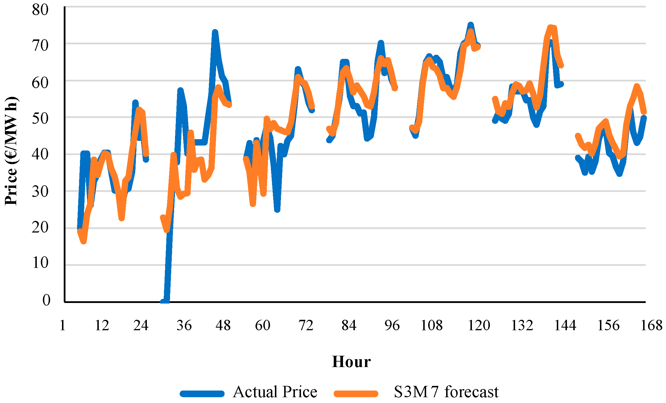
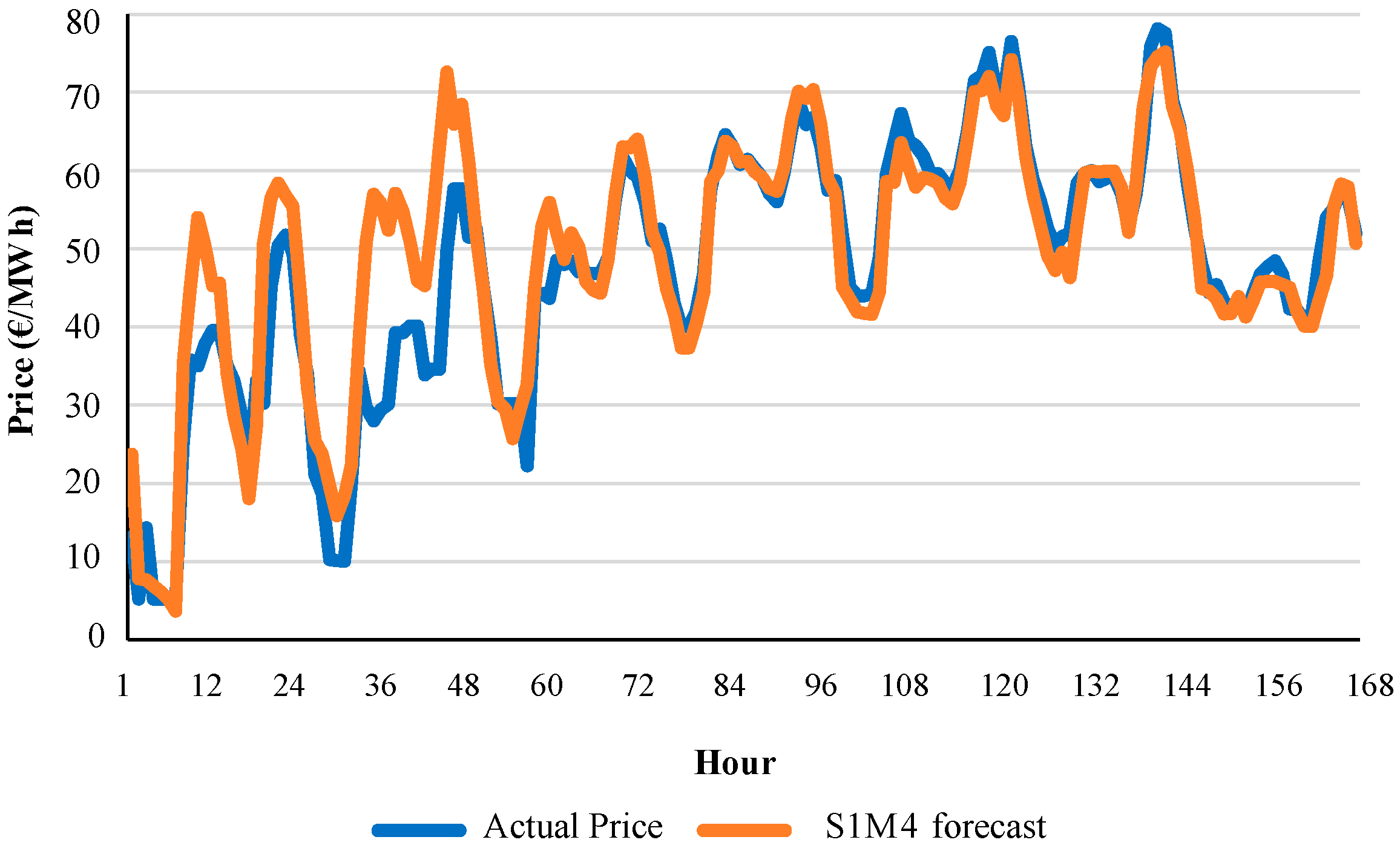
Figure 7 shows an example of the hourly evolution of actual price values and forecast values of model S1M4 for week 7 of year 2013.

5.2. Intraday Market Session 2

Let consider the possibility that variable V17I (the price D + 1 of intraday session 1 of the MIBEL) is available for ISMPF models for intraday market session 2. Models S2M2 to S2M5 of Table 9 tested the integration of each individual price variable (variables V3, V4, V5I and V17I) within baseline model S2M1. Thus, variable V3 (hourly price D) in model S2M2 (error of 16.71%) is clearly preferred with respect to variable V4 (hourly price D − 6) in model S2M3 (error of 19.61%). By integrating variables V5I (hourly price D + 1 of daily session) or V17I (hourly price D + 1 of intraday session 1) in model S2M1, model S2M4 led to an error of 9.84% and model S2M5 to 9.95%. 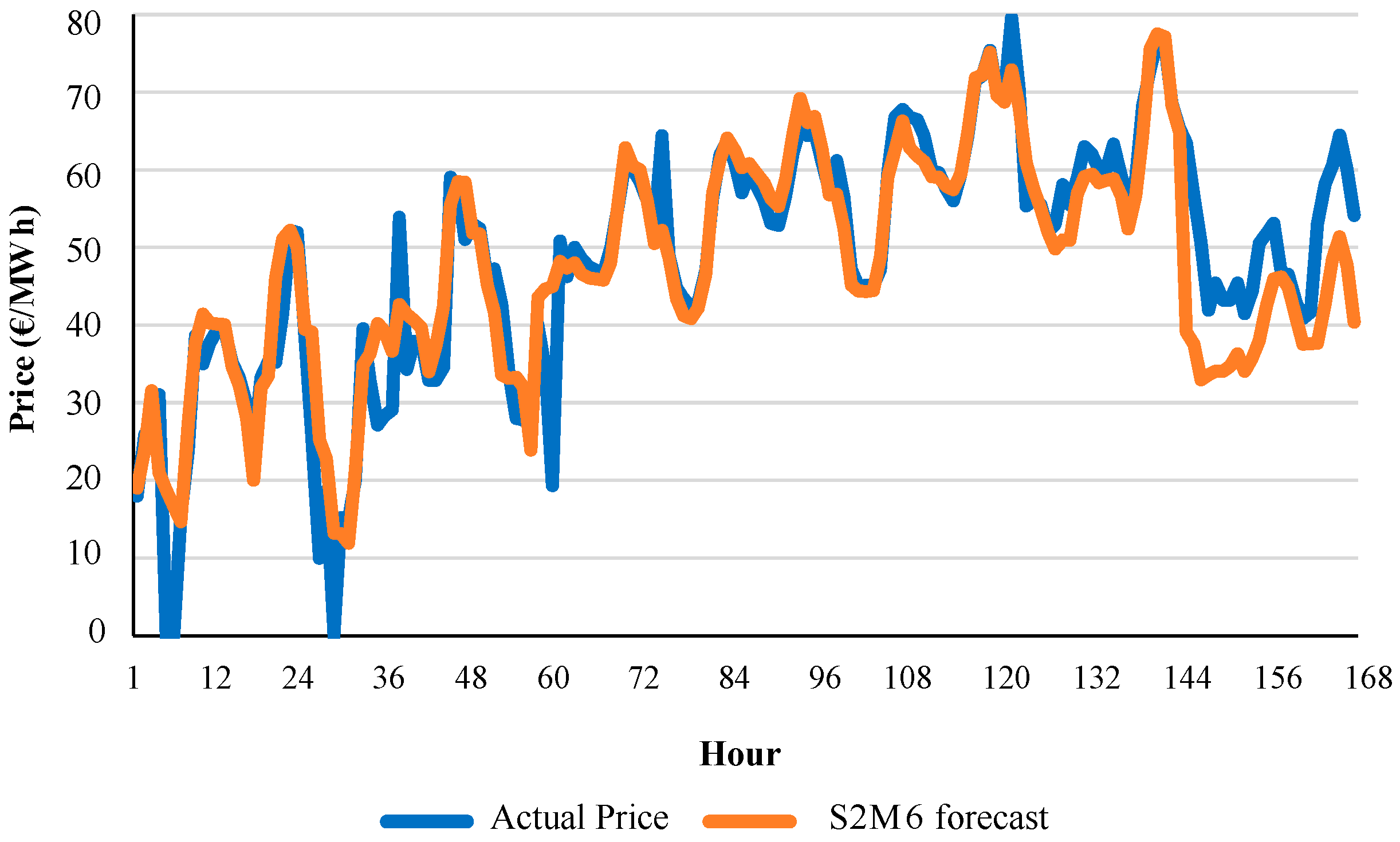Combining the two variables V5I and V17I with the variables of model S2M1, model S2M6 achieved the best MAPE of 8.85% among ISMPF models of intraday session 2. Please note that the performance of this model S2M6 (error of 8.85%) was higher than the best model S1M4 of intraday market session 1 (error of 7.49%).

The variable sets related to power demand (V6I and V7I) were tested following a procedure similar to that used for ISMPF models for intraday session 1; an error of 8.90% was obtained with model S2M7. Variables V8I to V11I (forecasted hourly weather variables D + 1 and forecasted hourly wind power generation D + 1) led to an error of 9.03% with model S2M8; and variables V12I to V16I (power generations D − 1) obtained an error of 9.16% with model S2M9. All these variables (V6I, V7I to V11I and V12I to V16I) did not achieve a better performance than the best model S2M6 (with a MAPE of 8.85%).

The best forecast error of 8.85% in model S2M6 for intraday market session 2 was higher than the best forecast error of 7.49% in model S1M4 for intraday market session 1. However, model S2M6 for intraday market session 2 still presented a significantly better performance than the best model for the daily session (model M18, with an error of 10.69% as shown in Table 5).

Figure 8 shows an example of the hourly evolution of actual price values and forecast values of model S2M6 for week 7 of year 2013.

5.3. Intraday Market Session 3

Let us consider that variable V17I (hourly price D + 1 of intraday session 1) and variable V18I (hourly price D + 1 of intraday session 2) can be available for ISMPF models for intraday market session 3. By applying similar procedures to those used for intraday sessions 1 and 2, the integration of individual price variables (variables V3, V4, V5I, V17I and V18I) of Table 10 within baseline model S3M1 was evaluated. Variables V5I, V17I and V18I led to better MAPEs of models S3M4 to S3M6 (MAPEs between 10.98% and 9.40%) with respect to models S3M2 and S3M3. The best combination of price variables, that is, variables V5I, V17I and V18I, was obtained in model S3M7 for intraday session 3 with a MAPE of 9.30%.

The inclusion of variables V6I and V16I with the variables of model S3M7 did not achieve improvements in the error (10.31% of model S3M8). The integration of variables V8I to V11I in model S3M9 obtained an error of 9.70%; the integration of variables V12I to V16I in model S3M10 led to an error of 10.09%.

Figure 9 shows an example of the hourly evolution of actual price values and forecast values of model S3M7 for week 7 of year 2013.

5.4. Intraday Market Session 4

Let us consider that variables V17I, V18I and V19I (hourly prices D + 1 of intraday sessions 1, 2 and 3) are available for ISMPF models for intraday market session 4. The analysis of the inclusion of individual variables V5I, V17I, V18I and V19I with chronological variables V1 and V2 of baseline model S5M1 showed that the best model is model S4M8 with a MAPE 9.08%, as shown in Table 11. This best model follows the pattern of variable combinations of ISMPF models for previous intraday sessions.

Again, variables V6I and V7I (power demand variables), variables V8I to V11I (forecasted variables) and variables V12I to V16I (power generations) did not improve the MAPE achieved by model S4M8, since they led to errors of 9.31% (model S4M9), 9.37% (model S4M10) and 9.49% (model S4M11).

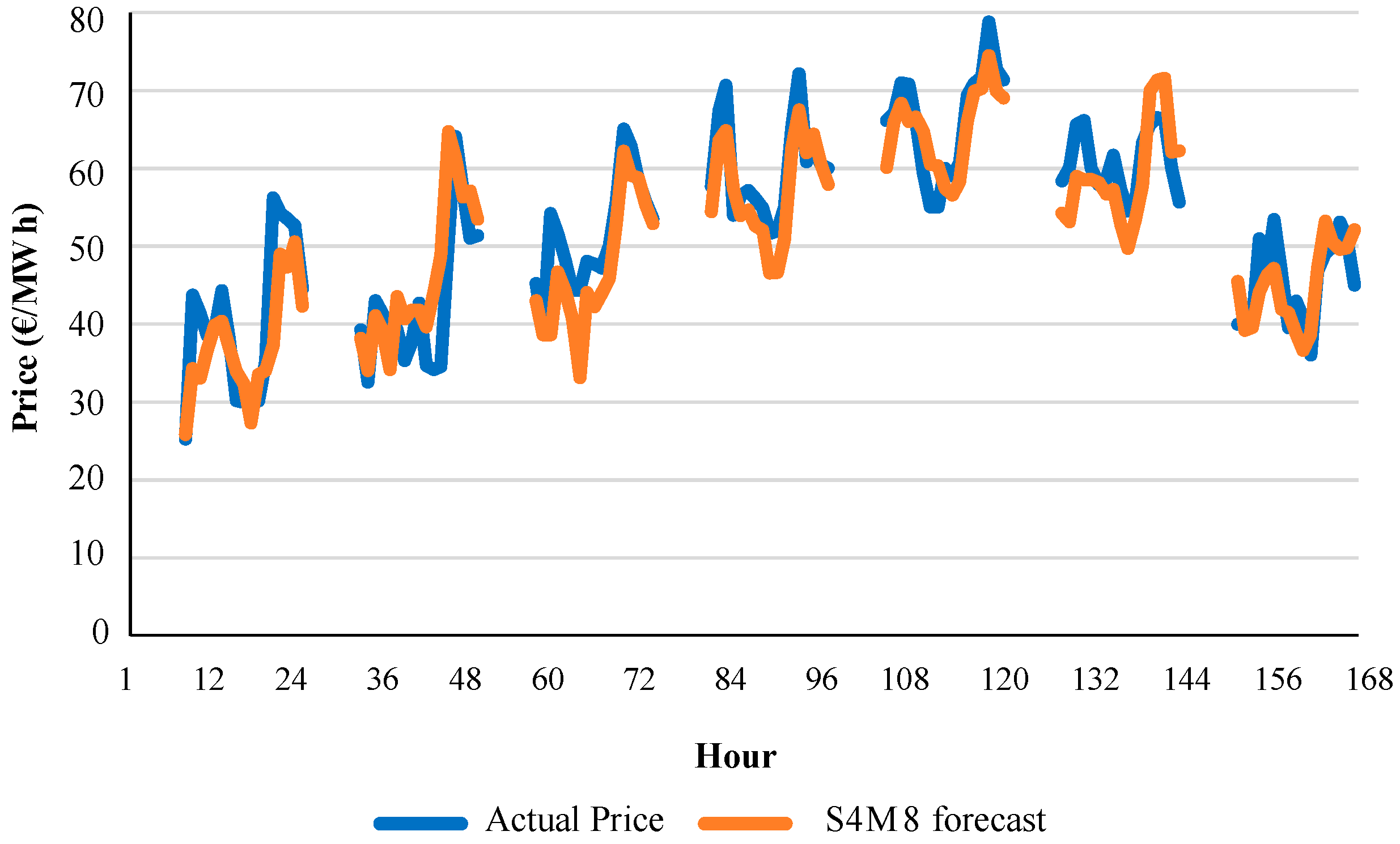
Figure 10 shows an example of the hourly evolution of actual price values and forecast values of model S4M8 for week 7 of year 2013.

5.5. Intraday Market Session 5

Let us consider that variables V17I to V20I (hourly prices D + 1 of intraday sessions 1 to 4) are available for ISMPF models for intraday market session 5. ISMPF models for intraday session 5 follow a similar pattern of variable combinations of ISMPF models for previous intraday sessions. The best ISMPF model is S5M9 with a MAPE of 9.52%, as shown in Table 12.

A MAPE of 12.17% was obtained with model S5M4 by using information from the daily session (variable V5I) in Table 12; an error of 11.47% with model S5M5 when using information from intraday session 1 (variable V17I); 11.07% with model S5M6 by using information from intraday session 2 (variable V18I); 10.40% with model S5M7 by using information from intraday session 3 (variable V19I); and an error of 10.18% was obtained with model S5M8 when using information from intraday session 4 (variable V20I). Therefore, the evolution of the MAPE from model S5M4 to model S5M8 in Table 12 indicates a progressive reduction in the forecasting error with the use of more updated information (hourly price D + 1 of the previous intraday sessions).

The integration of variables V6I and V7I in model S5M10 resulted in a MAPE of 9.53%. The consideration of variables V8I to V11I in model S5M11 led to an error of 9.69%. The inclusion of variables V12I to V16I in model S5M12 achieved an error of 10.16%. All these error values obtained by including additional variables V6I, V7I, V8I to V11I, and V12I to V16I to model S5M9 were higher than the error (9.52%) of the best ISMPF model (model S5M9) for intraday session 5.

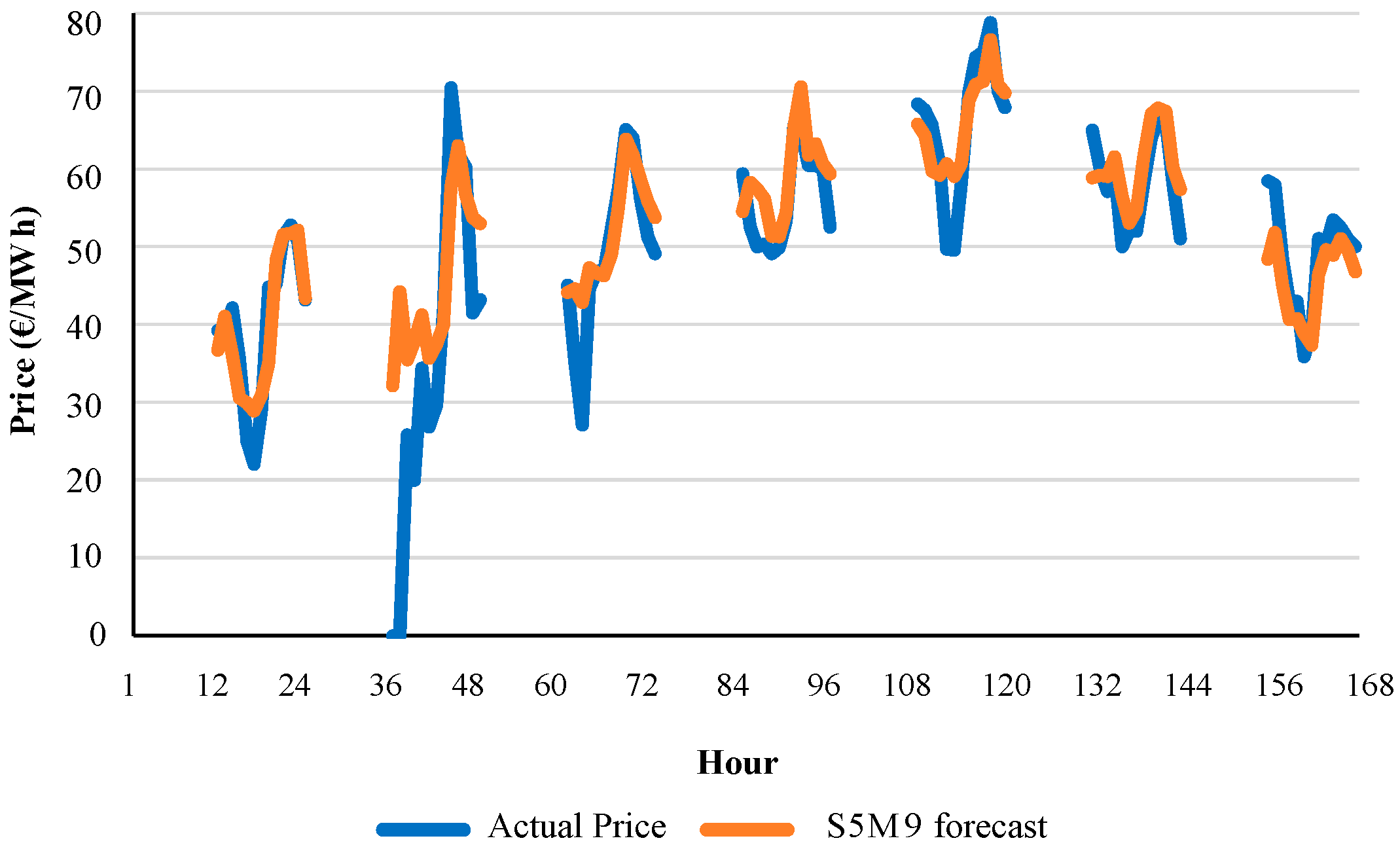
Figure 11 shows an example of the hourly evolution of actual price values and forecast values of model S5M9 for week 7 of year 2013.

5.6. Intraday Market Session 6

Let consider that variables V17I to V21I (hourly prices D + 1 of intraday sessions 1 to 5) are available for ISMPF models for intraday market session 6. ISMPF models for intraday session 6 follow a different pattern of variable combinations from that of ISMPF models for previous intraday sessions. As shown in Table 13, there are eight possible price variables: price D (variable V3); price D − 6 (variable V4); price D + 1 of daily session (variable V5I); and prices D + 1 of previous intraday sessions 1 to 5 (variables V17I to V21I). Variables V3 and V4 in models S6M2 and S6M3 improved the MAPE with respect to that of model S6M1. The evolution of the MAPE from model S6M4 to model S6M9 in Table 13, with a reduction from 15.35% of model S6M4 to 12.73% of model S6M9, indicates a progressive decrease in the MAPE due to the inclusion of more updated information.

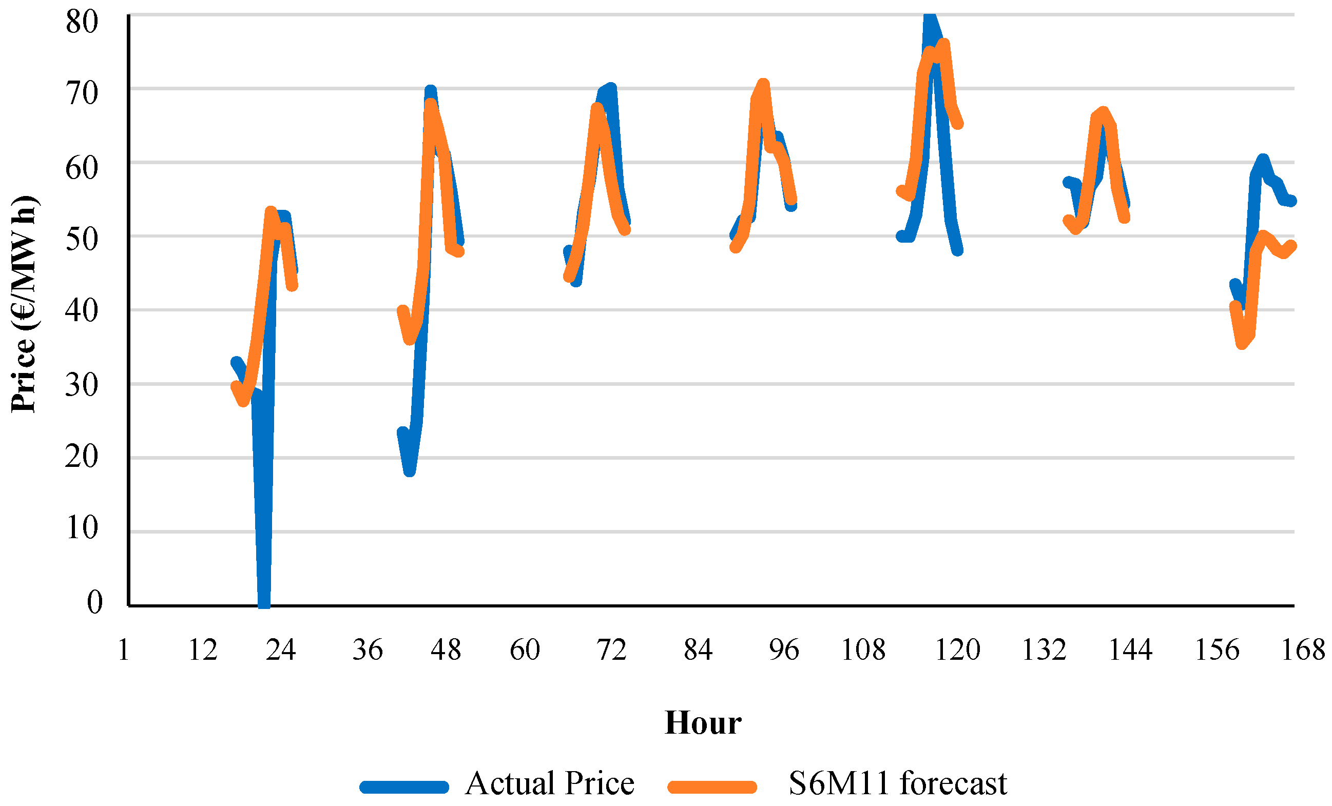
On the contrary to previous intraday sessions, the best ISMPF model for intraday session 6 does not use the combination of all the price D + 1 variables of previous intraday sessions and the price D + 1 of the daily session. The best MAPE of 12.48% was achieved with model S6M11 by including variables V19I to V21I corresponding to the previous three intraday sessions (intraday sessions 3, 4 and 5).

A suitable analysis, similar to that carried out for the other intraday sessions, allowed to determine that model S6M15 (including variables V6I and V7I) led to a higher MAPE (12.78%) than error 12.48% of the best model S6M11; model S6M16 (adding variables V8I to V11I) obtained an error of 13%; and model S6M17 (including variables V12I to V16I) resulted in an error of 13.99%.

Figure 12 shows an example of the hourly evolution of actual price values and forecast values of model S6M11 for week 7 of year 2013.

5.7. Comparison of the Best ISMPF Models with the Best DSMPF Model

Table 14. The best ISMPF models and the best DSMPF model.

Forecasting Session for MIBEL	Forecasting Period	Best Forecasting Model	MAPE (%)
Daily session	0 h (D + 1) to 23 h (D + 1)	M18	10.69
Intraday session 1	21 h (D) to 23 h (D + 1)	S1M4	7.49
Intraday session 2	0 h (D + 1) to 23 h (D + 1)	S2M6	8.85
Intraday session 3	4 h (D + 1) to 23 h (D + 1)	S3M7	9.30
Intraday session 4	7 h (D + 1) to 23 h (D + 1)	S4M8	9.08
Intraday session 5	11 h (D + 1) to 23 h (D + 1)	S5M9	9.52
Intraday session 6	15 h (D + 1) to 23 h (D + 1)	S6M11	12.48

shows the best ISMPF models and the best DSMPF model, including the corresponding main characteristics and the MAPEs. The error increased from the best model S1M4 of intraday session 1 (error of 7.49%) to the best model S6M11 for intraday session 6 (error of 12.48%). Error 10.69% of model M18 (the best DSMPF model) was higher than most of the errors of the best ISMPF models for intraday sessions (intraday sessions 1 to 5), although the main characteristics of the best ISMPF models for intraday sessions were different from those of the best DSMPF model for the daily session.

6. Conclusions

This paper presents novel ISMPF models for hourly price forecasting of the six intraday sessions of the MIBEL as well as a systematic analysis of the MAPEs corresponding to suitable combinations of their input variables in order to determine the best ISMPF model for each of the sessions, that is, the best combination of input variables for ISMPF models in each intraday session.

The methodology of the analysis is initially applied to DSMPF for the day-ahead hourly price forecasting, in the daily session of the MIBEL, and also applied to RMPE models for the estimation of the hourly prices.

DSMPF models use as input variables (price explanatory variables) recorded time series of hourly prices in previous days, regional-aggregated hourly power demands and hourly power generations of most of the types of electricity production in the previous day, forecasts of demand, wind power generation and weather (hourly wind speed, temperature and irradiation) for the day-ahead in the region, and chronological variables.

The main difference between the RMPE models and DSMPF models is that RMPE models use actual power generation values and actual power demand values of the day-ahead instead of the values of these variables on the previous day. Thus, RMPE models are not models for price forecast, but for price estimation.

Both DSMPF and RMPE models were satisfactorily applied to the real-life case study of the MIBEL that covers the mainland of Portugal and Spain. Descriptive statistics of price data have been provided. The MAPE of the best RMPE model was 9.9%; it represents the lowest limit of the MAPE of any RMPE model for price estimation or any DSMPF model for price forecast, using the same kind of input variables of RMPE models.

The MAPE of the best DSMPF model (model M18) was 10.7%, very close to the “minimum error” (9.9%) obtained by the best RMPE model, showing a very satisfactory performance of the best DSMPF model.

The ISMPF models consider the input variables included in DSMPF models as well as the hourly prices of the daily session and hourly prices of previous intraday sessions of the MIBEL. The methodology of the analysis used for DSMPF models is also applied to ISMPF models to find the combination of input variables that achieves the best MAPE for each intraday session of the MIBEL in order to determine the best ISMPF model.

The MAPE varied from 7.49% of the best ISMPF model (model S1M4) for the intraday session 1 to 9.52% of the best ISMPF model (model S5M9) for the intraday session 5; it raised to 12.48% of the best ISMPF model (model S6M11) for the intraday session 6. Thus, the MAPE of the best ISMPF models for intraday sessions 1 to 5 were clearly better than the error of 10.7% of the best DSMPF model.

The best ISMPF models for intraday sessions 1 to 5 use only the hourly prices of the daily session and hourly prices of previous intraday sessions, as well as chronological variables, and they are therefore significantly simpler than the best DSMPF model. On the other hand, the best ISMPF model of intraday session 6 exclusively utilizes the hourly prices of previous intraday sessions 3, 4 and 5, and the chronological variables, and it is also considerably simpler than the best DSMPF model.

The best Intraday Session Model for Price Forecasts of this paper, their performance in the MIBEL mainly in terms of MAPE, and the determination of their best input variables can be useful for agents of the electricity intraday market and the electric energy industry.