Article

Mid-Term Electricity Market Clearing Price Forecasting with Sparse Data: A Case in Newly-Reformed Yunnan Electricity Market

Institute of Hydropower System & Hydroinformatics, Dalian University of Technology, Dalian 116024, China
*
Author to whom correspondence should be addressed.
Energies 2016, 9(10), 804; https://doi.org/10.3390/en9100804
Submission received: 16 June 2016 / Revised: 18 September 2016 / Accepted: 27 September 2016 / Published: 8 October 2016
(This article belongs to the Special Issue Forecasting Models of Electricity Prices)

Abstract

:
For the power systems, for which few data are available for mid-term electricity market clearing price (MCP) forecasting at the early stage of market reform, a novel grey prediction model (defined as interval GM(0, N) model) is proposed in this paper. Over the traditional GM(0, N) model, three major improvements of the proposed model are: (i) the lower and upper bounds are firstly identified to give an interval estimation of the forecasting value; (ii) a novel whitenization method is then established to determine the definite forecasting value from the forecasting interval; and (iii) the model parameters are identified by an improved particle swarm optimization (PSO) instead of the least square method (LSM) for the limitation of LSM. Finally, a newly-reformed electricity market in Yunnan province of China is studied, and input variables are contrapuntally selected. The accuracy of the proposed model is validated by observed data. Compared with the multiple linear regression (MLR) model, the traditional GM(0, N) model and the artificial neural network (ANN) model, the proposed model gives a better performance and its superiority is further ensured by the use of the modified Diebold–Mariano (MDM) test, suggesting that it is suitable for mid-term electricity MCP forecasting in a data-sparse electricity market.

1. Introduction

Electricity price is one of the most important parameters of deregulated and competitive electricity markets; wherein, the electricity market clearing price (MCP) is the final outcome of the market bid price and generally determined by the aggregated demand and supply bid curves, which exists when an electricity market is clear of shortage and surplus. On 15 March 2015, the Communist Party of China (CPC) Central Committee and State Council’s opinions on further deepening the reforms of the electric power system [1] marked the beginning of new electricity market reform in China, after Investment Decentralization in 1986, Unbundling of Government Admin and Business Operation in 1997 and Unbundling of Generation and Transmission in 2002 [2]. Unlike mature electricity markets in other countries, to guarantee the security and stability operation at the early stage of reform, the Chinese electricity market mainly comprises the mid- and long-term exchanges so far. Therefore, the mid-term electricity MCP forecasting has become one of the most concerning issues, as it is essential for resource reallocation, maintenance scheduling, financial risk reducing, bilateral contracting, budgeting and planning purposes [3].
Over the last 15–20 years, electricity price forecasting (EPF) has been carried out with various methods, bringing a variety of success. Till now, there is no consensus criterion on the classification of these models [4,5]. To our knowledge, they can be mainly classified into the following categories: (1) equilibrium and simulation models, such as the Nash–Cournot model [6,7,8], production-cost models (PCM) [9], strategic PCM (SPCM) [10], and so on; (2) statistical methods, such as multiple regression [11], exponential smoothing [12,13], time series [14,15,16], wavelet transform (WT) [17,18,19], AR-type models ( such as auto-regressive moving average (ARMA) [16], auto-regressive integrated moving average (ARIMA) [20,21], seasonal ARIMA (SARIMA) [22]), and so on; (3) artificial intelligence models, such as artificial neural network (ANN) [23,24], support vector machine (SVM) [25,26] and data mining models [27,28]; and (4) hybrid models, which combine two or more single methods or models described above [29,30,31]. According to these research works, most works are focused on short-term EPF, commonly known as day-ahead EPF. In contrast, not much has been performed in the mid-term horizon [3,32,33,34,35]. Compared to short-term forecasting, mid-term forecasting is much more challenging. This is because the prediction horizon is much longer, and the price may not be contiguous to the immediate past periods, which means the trend information of the immediate past is not as valuable as for short-term forecasting. In addition, the influence factors of mid-term EPF are various and, worse, some are unavailable. When it comes to the newly-reformed electricity market in China, being at the early stage, another bigger challenge is how to build accurate models with relatively few available samples, which is beyond the capability of most forecasting models above. Appropriate prediction models need to be studied.
In systems theory, if the description of a system is completely known, it is known as a white system. In contrast, a black-box system means that it is completely unknown. When in an intermediate state, it is called a grey system [36]. The grey system theory (GST) was firstly proposed by Deng in 1982 [37], and several grey prediction models were created later. For the grey model, it is characterized by its prominent capability in modeling with small samples and poor information, which commonly exist in the natural world. Thus, it has been successfully employed in various fields and demonstrated satisfactory results, such as social [38,39], economic [40,41], agricultural [42], industrial [43], etc. The electricity MCP is a synthetic variable of the market mechanism with many uncertainties, obviously in accordance with the characteristics of GST, so the electricity MCP forecasting is adapted to be solved through grey prediction models. Furthermore, as the mid-term electricity MCP is not closely related to the immediate past periods and affected by multiple factors, a widely-used static multi-variable grey prediction model in GST named GM(0, N) is concerned in this paper. However, to directly forecast the mid-term electricity MCP, there are some difficulties or disadvantages in the traditional GM(0, N) model, including:
  • The input variables of the model would affect the forecasting result directly. Thus, the selection of appropriate influence factors of electricity MCP is extremely important, but also tough, as it varies from different electricity markets.
  • The mid-term electricity MCP is obviously volatile in nature and out of a monotonous trend. The forecasting accuracy is unsatisfactory when the value of the next forecasting point is away from the fitting model constructed only with known data.
  • The least square method (LSM) used in the traditional GM(0, N) model to identify parameters is effective on condition of the existence of the inverse of matrix B T B , but this does not work when B T B is a singular matrix in some cases.
To overcome these problems and achieve a successful implementation for mid-term electricity MCP forecasting with few available data, a novel grey prediction model defined as the interval GM(0, N) model is proposed in this paper. The main contributions of this work can be summarized as follows:
  • Based on depth analysis of the newly-reformed electricity market, the influence factors of electricity MCP are studied, and input variables are carefully selected according to three aspects: supply factors, demand factors and supplemented factors.
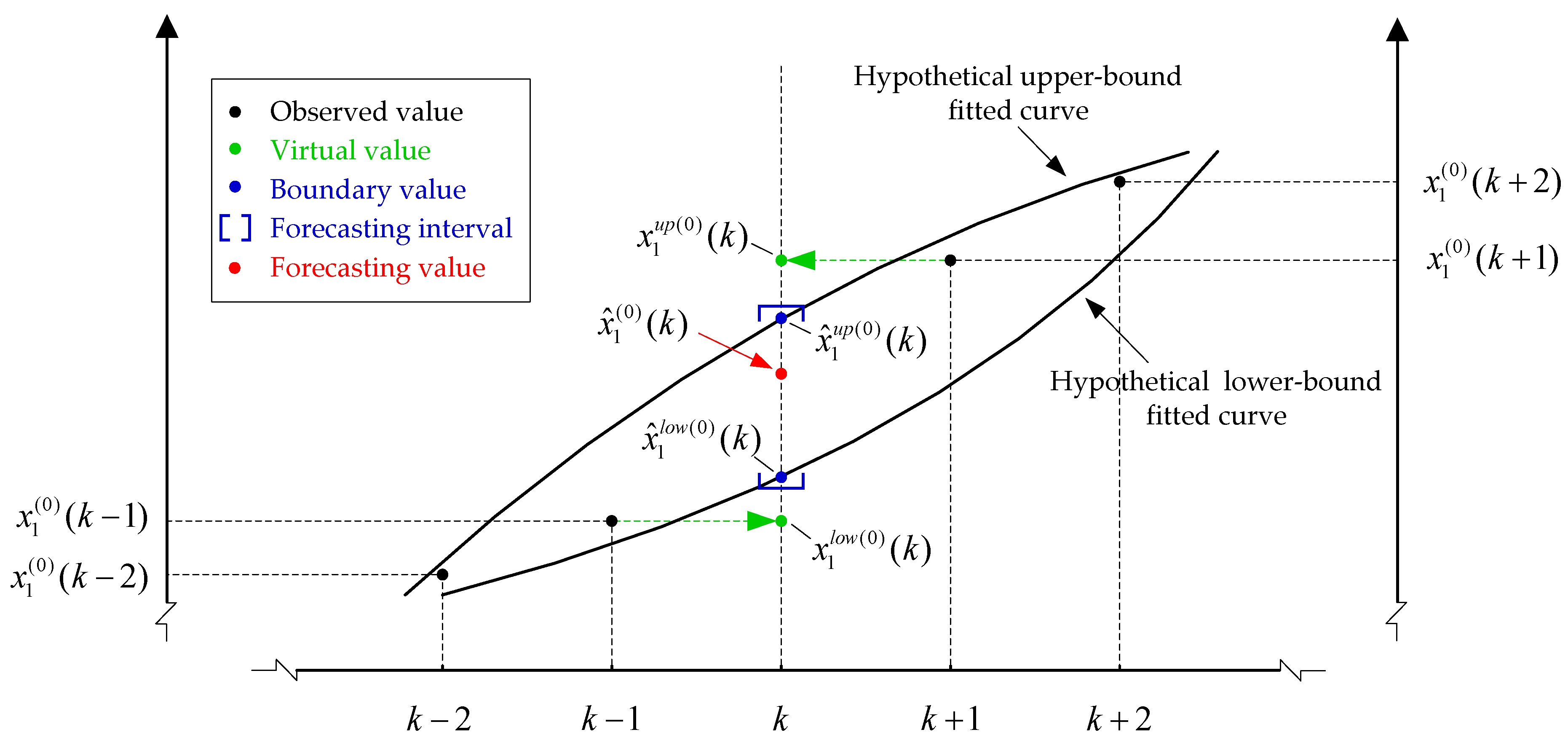
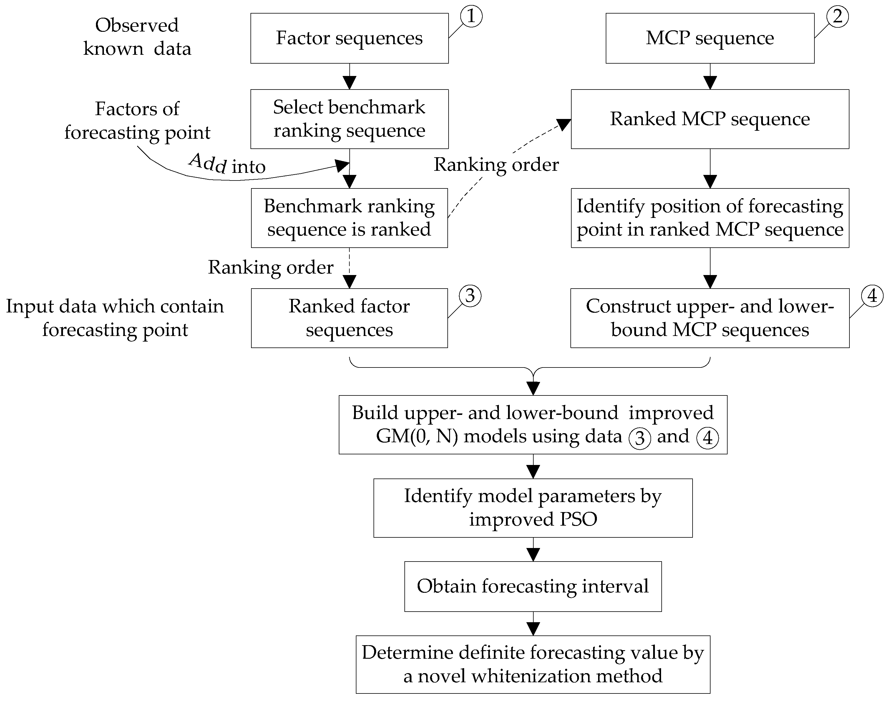
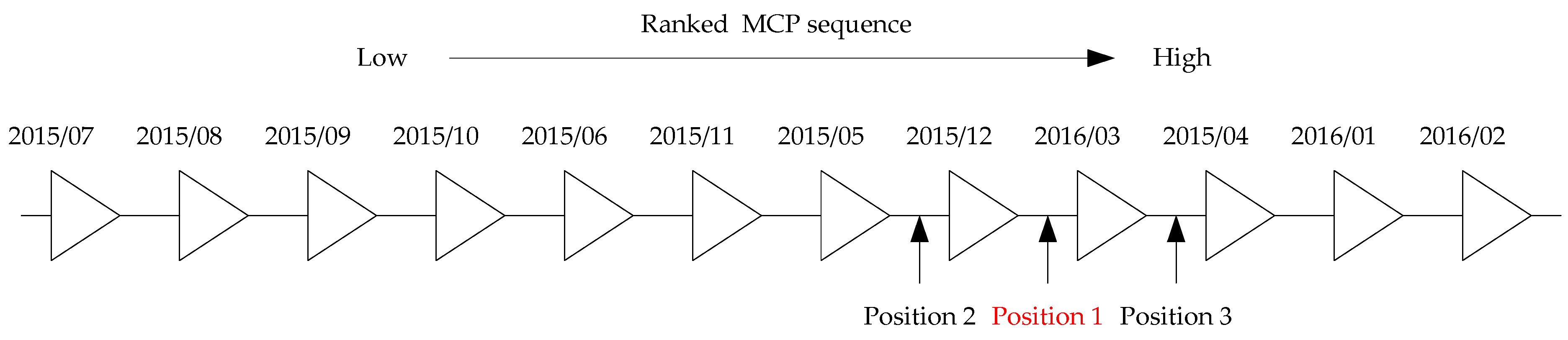
  • In the proposed interval GM(0, N) model, two improved GM(0, N) models are included, respectively estimating the upper and lower bounds of the forecasting value. Firstly, to reduce randomness and increase smoothness, all input sequences (not containing values of the next forecasting point) including the MCP sequence and factor sequences are ranked in accordance with the ascending order of the MCP sequence. Then, one of the factor sequences is selected as the benchmark ranking sequence according to its ranking order and correlation with the MCP sequence. The position of the forecasting point in the ranked MCP sequence thus can be determined by sorting the benchmark ranking sequence, which contains the factor value of the forecasting point. Finally, two neighboring (upper and lower) points of the forecasting point in the ranked MCP sequence are regarded as two virtual values to construct two new MCP sequences, which are respectively used as characteristic sequences for two improved GM(0, N) models, obtaining the forecasting interval. In the two improved GM(0, N) models, the input sequences used for building the model include not only known data, but also the virtual MCP and predicted influence factors of the forecasting point.
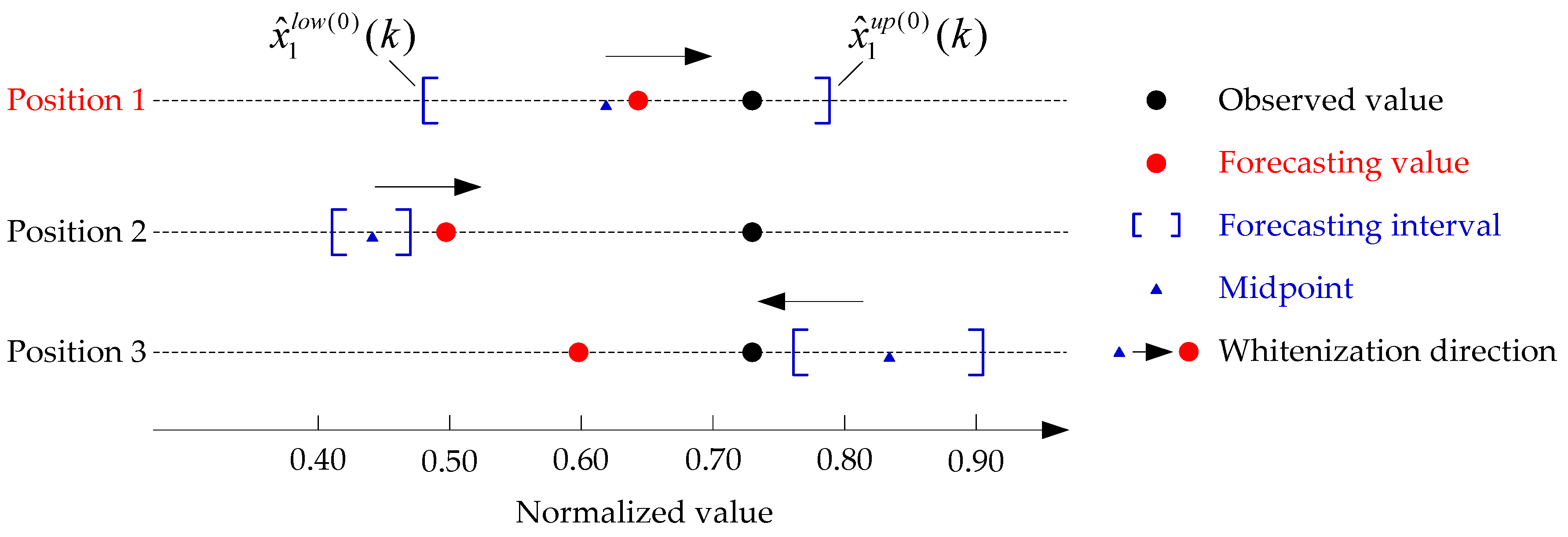
  • Based on the forecasting interval, a novel whitenization method considering correlations between electricity MCP and influence factors is established to determine the definite forecasting value.
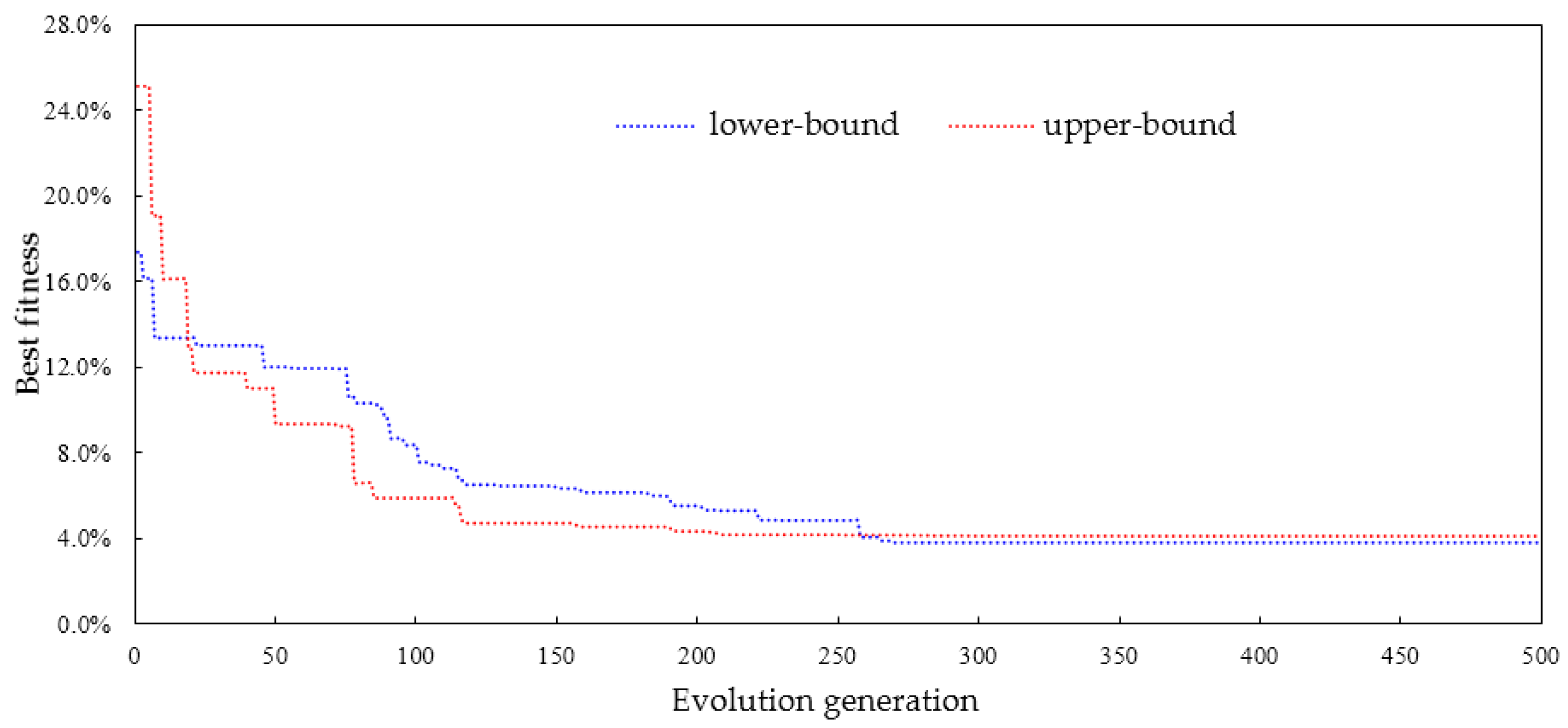
  • The parameters of the GM(0, N) model are identified by an improved particle swarm optimization (PSO) instead of LSM.
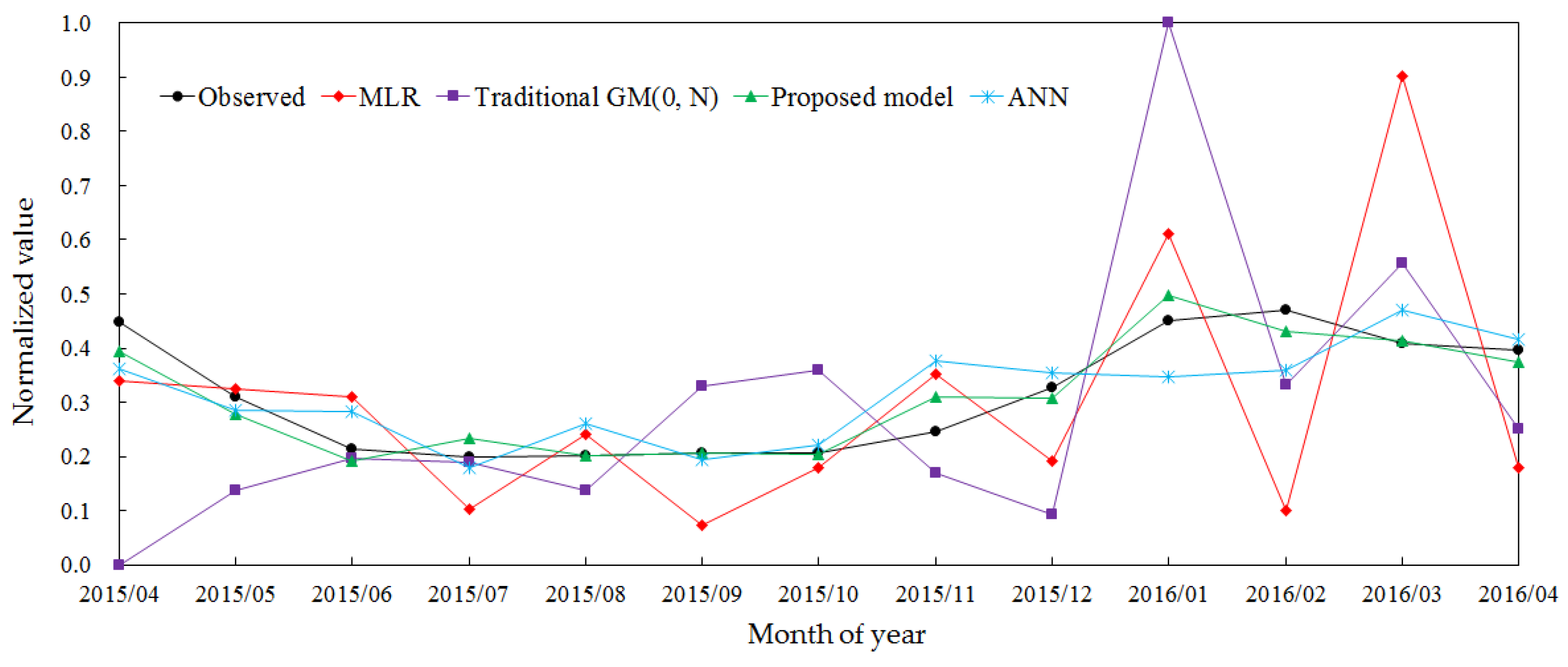
  • The performance of the proposed model has been validated by applying it to the newly-reformed Yunnan electricity market. Further comparisons between the proposed model and other models, including the multiple linear regression (MLR) model, the traditional GM(0, N) model and the artificial neural network (ANN) model, are carefully discussed and also evaluated by using the modified Diebold–Mariano (MDM) test. The results indicate that the proposed model is an effective means of mid-term electricity MCP forecasting with sparse data.
The remainder of this paper is organized as follows. In Section 2, the method and theory are introduced. Section 3 is devoted to the detailed presentation of the proposed model. In Section 4, electricity market conditions are analyzed, and input variables are selected. In Section 5, the case study and forecasting results are carefully discussed. Finally, Section 6 outlines the main conclusions.

2. Method and Theory

2.1. Principle of the Traditional GM(0, N) Model

Set X 1 ( 0 ) = { x 1 ( 0 ) ( 1 ) , x 1 ( 0 ) ( 2 ) , , x 1 ( 0 ) ( n ) } as the raw characteristic sequence (here, the electricity MCP sequence); n is the data length. Set X i ( 0 ) = { x i ( 0 ) ( 1 ) , x i ( 0 ) ( 2 ) , , x i ( 0 ) ( n ) } , i I , I = { 2 , 3 , , N } as the relevant factor sequences (here, the influence factors of mid-term electricity MCP); N is the number of all sequences, and the total number of factor sequences is N 1 . Therefore, the AGO (accumulated generation operation) sequence X i ( 1 ) = { x i ( 1 ) ( 1 ) , x i ( 1 ) ( 2 ) , , x i ( 1 ) ( n ) } is firstly generated by Equation (1).
x i ( 1 ) ( k ) = m = 1 k x i ( 0 ) ( m ) , ( k = 1 , 2 , , n ;   i = 1 , 2 , , N )
Then, call formula Equation (2):
x 1 ( 1 ) ( k ) = i = 2 N b i x i ( 1 ) ( k ) + a , ( k = 1 , 2 , , n )
as the traditional GM(0, N) model. Where, b i and a are identified parameters, which can be solved by the least square method (LSM), if the inverse of matrix B T B exists. That is:
P 0 N = [ b 2 , b 3 , , b N , a ] T = ( B T B ) 1 B T y N
where, B = [ x 2 ( 1 ) ( 1 ) x 3 ( 1 ) ( 1 ) x N ( 1 ) ( 1 ) 1 x 2 ( 1 ) ( 2 ) x 3 ( 1 ) ( 2 ) x N ( 1 ) ( 2 ) 1 x 2 ( 1 ) ( n ) x 3 ( 1 ) ( n ) x N ( 1 ) ( n ) 1 ] , y N = [ x 1 ( 1 ) ( 1 ) ,   x 1 ( 1 ) ( 2 ) ,   ,   x 1 ( 1 ) ( n ) , 1 ] T .
Thus, we can get the next forecasting value for the characteristic sequence by Equation (4).
{ x ^ 1 ( 0 ) ( 1 ) = x 1 ( 0 ) ( 1 ) x ^ 1 ( 0 ) ( k + 1 ) = x ^ 1 ( 1 ) ( k + 1 ) x ^ 1 ( 1 ) ( k ) ,   k = 1 , 2 , , n
where x ^ 1 ( 1 ) ( k + 1 ) is the forecasting value of x 1 ( 1 ) ( k + 1 ) ; x ^ 1 ( 0 ) ( k + 1 ) is the forecasting value of x 1 ( 0 ) ( k + 1 ) .

2.2. Limitation and Requirement for Implementation

2.2.1. Limitation of Least Square Method (LSM) in the Traditional GM(0, N) Model

In the traditional GM(0, N) model, parameters b i and a are identified by LSM, shown in Equation (3). However, this is conditioned on the existence of the inverse of matrix B T B .
Proof: The determinant of B T B is D e t ( B T B ) ; the inverse matrix of B T B exists only when:
D e t ( B T B ) 0
that is when the B is a column full rank matrix. That is when, for any constant u ( , + ) ,
X i ( 1 ) + u X j ( 1 ) 0 , ( i , j I , i j )
otherwise, the inverse of matrix B T B does not exist.
From the equations above, it can be observed that the limitation of LSM depends on the input dataset. However, Equation (6) does not hold for all cases, especially with the increasing length of available data. Therefore, the LSM cannot be adapted to identify parameters b i and a for the GM(0, N) model in some cases. To avoid any mistakes caused by this limitation and to ensure the general applicability of the model, the parameter identification method should be improved.

2.2.2. Requirements for Input Variables

Although the great feature of the GM(0, N) model is allowing the randomness of data sequences and modeling with small samples and poor conditions, the volatile nature of the electricity price has a negative effect on forecasting results. Despite the fact that AGO has been applied to convert the sequences to a monotonic increasing trend, the modeling accuracy is still limited by directly using raw known data. For better accuracy, the input data need to be pre-processed. Furthermore, the related influence factors of electricity MCP are various, and input variables should be carefully selected, as they also have an impact on the forecasting result.

2.3. Performance Evaluation

2.3.1. Checking Method of Grey Prediction Models

To evaluate the fitting precision of the proposed grey prediction model, two main parameters in the after-test residue checking method, posterior-error ( C ) and micro-error-probability ( P ), are adopted, respectively defined as:
C = S 2 S 1
P = p r o b a b i l i t y { | Δ x 1 ( 0 ) ( k ) Δ x ¯ 1 ( 0 ) ( k ) | < 0.6745 S 1 }
where:
{ S 1 = 1 n 1 k = 1 n [ x 1 ( 0 ) ( k ) x ¯ 1 ( 0 ) ( k ) ] 2 S 2 = 1 n 1 k = 1 n [ Δ x 1 ( 0 ) ( k ) Δ x ¯ 1 ( 0 ) ( k ) ] 2 x ¯ 1 ( 0 ) ( k ) = 1 n k = 1 n x 1 ( 0 ) ( k ) Δ x 1 ( 0 ) ( k ) = x 1 ( 0 ) ( k ) x ^ 1 ( 0 ) ( k ) Δ x ¯ 1 ( 0 ) ( k ) = 1 n k = 1 n Δ x 1 ( 0 ) ( k )
The fitting precision grade is shown in Table 1.

2.3.2. Performance Evaluation of Forecasting Models

For evaluating electricity MCP forecasting values, mean absolute error (MAE), mean squares error (MSE) and mean absolute percentage error (MAPE) are the most widely-used measurements, respectively shown in Equations (10)–(12). The smaller the MAE, MSE and MAPE, the better forecasting performance the model shows.
M A E = 1 n k = 1 n | x 1 ( 0 ) ( k ) x ^ 1 ( 0 ) ( k ) |
M S E = 1 n k = 1 n [ x 1 ( 0 ) ( k ) x ^ 1 ( 0 ) ( k ) ] 2
M A P E = 1 n k = 1 n | x 1 ( 0 ) ( k ) x ^ 1 ( 0 ) ( k ) x 1 ( 0 ) ( k ) | × 100 %
To further judge the forecasting performances of different forecasting models from a statistical point of view, a statistical evaluation method named modified Diebold–Mariano (MDM) test [44] is also proposed. The MDM test is an extension of the Diebold–Mariano test [45] and has been widely used in forecasting research. The MDM test statistic for the h-step ahead forecast is specified as:
M D M = [ n + 1 2 h + n 1 h ( h 1 ) n ] 1 2 [ V ( d ¯ ) ] 1 2 [ d ¯ ]
where V ( d ¯ ) = [ n 1 ( γ 0 + 2 k = 1 h 1 γ k ) ] is the variance of d ¯ ; γ k = n 1 t = k + 1 n ( d t d ¯ ) ( d t k d ¯ ) is the k -th autocovariance of d t ; d ¯ = n 1 t = 1 n d t is the mean of d t ; d t = L ( e 1 , t ) L ( e 2 , t ) ,   t = 1 , 2 , 3 , , n is the loss differentials; L ( e i , t ) is the loss function of forecast error e i , t , i = 1 , 2 ; e i , t = x t x ^ i , t , x t denotes the actual data series, and x ^ i , t denotes the forecasting series of forecasting model i . In our study, the popular loss functions used in power systems, i.e., the MAE and MSE loss functions, are adopted. Under the null hypothesis of the equal forecasting performances of forecasting models, the MDM test statistic follows a t-distribution with (n − 1) degrees of freedom, so that tests can be carried out. As the detailed principle of the MDM test can be easily found in related papers, we will not repeat it here.

3. Novel Interval GM(0, N) Model

Sorting is a common way to get a descending (or ascending) sequence. However, the position of the forecasting point in the MCP sequence cannot be obtained, as its actual value is unknown. For this, one of the factor sequences is selected as the benchmark ranking sequence to determine the position of the forecasting point in the MCP sequence. Then, the actual value of the forecasting point is respectively replaced by its two neighboring (upper and lower) values in the MCP sequence. Two new MCP sequences thus are constructed, which are respectively used as the characteristic sequence for two improved GM(0, N) models, obtaining the upper and lower bounds of the forecasting value (i.e., forecasting interval). Furthermore, the model parameters are identified by an improved PSO instead of LSM. Finally, the definite forecasting value is believed to be related to this forecasting interval and further determined by a novel whitenization method. In this section, the implementation of this improved grey prediction model (defined as the interval GM(0, N) model) is given in detail.

3.1. Selection of the Benchmark Ranking Sequence

The factor sequence that shares the most similarities with the characteristic sequence is selected to help with determining the position of the forecasting point in the MCP sequence. The chosen factor sequence is called the benchmark ranking sequence, and the steps are given below.
Step 1. Get factor sequences that have the same (or reverse) ranking order as the characteristic sequence, defined as X i s u b ( 0 ) . Two sequences X = ( x 1 ,   , x k , , x n ) and Y = ( y 1 ,   , y k , , y n ) are regarded as having the same (or reverse) ranking order, if:
(1)
The lengths of X and Y are equal.
(2)
A new sequence X ˜ = { x 1 , , x k , , x n } is obtained by ranking X in ascending order of value. Corresponding with the same index of the subscript, Y ˜ = { y 1 , , y k , , y n } is formed. For any k , there is y k y k 1 0 (or < 0 ).
Similarly, the factor sequences X i s u b ( 0 ) can be obtained, i I s u b , I s u b I .
Step 2. The correlation coefficient r 1 , i between X 1 ( 0 ) and X i ( 0 ) is calculated by correlation analysis, shown in Equation (14).
r 1 , i = r ( X 1 ( 0 ) , X i ( 0 ) ) = k = 1 n ( x 1 ( 0 ) ( k ) x ¯ 1 ( 0 ) ) ( x i ( 0 ) ( k ) x ¯ i ( 0 ) ) k = 1 n ( x 1 ( 0 ) ( k ) x ¯ 1 ( 0 ) ) k = 1 n ( x i ( 0 ) ( k ) x ¯ i ( 0 ) ) , ( i I )
where x ¯ i ( 0 ) = 1 n k = 1 n x i ( 0 ) ( k ) is the mean value of X i ( 0 ) . Then, the benchmark ranking sequence (define its index in factor sequences as τ ) is determined by the following rules: if I s u b , τ is the index when r 1 , τ = MAX i I s u b { r 1 , i } , else if I s u b = , τ is the index when r 1 , τ = MAX i I { r 1 , i } . Therefore, the characteristic sequence and factor sequences are ranked in accordance with the ascending or descending order of the benchmark ranking sequence. In what follows, sequences mean ranked sequences.

3.2. Calculation for Forecasting Interval

By comparing the corresponding factor value of the forecasting point in the benchmark ranking sequence, the position of the forecasting point can be obtained, which is also regarded as the position in the ranked MCP sequence. Suppose the position is k ; the ranked MCP sequence that contains the forecasting point is:
X 1 ( 0 ) = { x 1 ( 0 ) ( 1 ) , x 1 ( 0 ) ( 2 ) , , x 1 ( 0 ) ( k 1 ) , ( k ) , x 1 ( 0 ) ( k + 1 ) , , x 1 ( 0 ) ( n + 1 ) }
where the ( k ) is the point to be forecasted and the data length is changed from n to n + 1 . Defining the lower- and upper-bound virtual values of x 1 ( 0 ) ( k ) as x 1 l o w ( 0 ) ( k ) and x 1 u p ( 0 ) ( k ) , respectively. Therefore, the lower- and upper-bound MCP sequences can be constructed, respectively named as X 1 l o w ( 0 ) and X 1 u p ( 0 ) , and expressed as:
{ X 1 l o w ( 0 ) = { x 1 ( 0 ) ( 1 ) , x 1 ( 0 ) ( 2 ) , , x 1 ( 0 ) ( k 1 ) , x 1 l o w ( 0 ) ( k ) , x 1 ( 0 ) ( k + 1 ) , , x 1 ( 0 ) ( n + 1 ) } X 1 u p ( 0 )   = { x 1 ( 0 ) ( 1 ) , x 1 ( 0 ) ( 2 ) , , x 1 ( 0 ) ( k 1 ) , x 1 u p ( 0 ) ( k ) , x 1 ( 0 ) ( k + 1 ) , , x 1 ( 0 ) ( n + 1 ) }
two neighboring (lower and upper) points of x 1 ( 0 ) ( k ) in the ranked MCP sequence, i.e., x 1 ( 0 ) ( k 1 ) and x 1 ( 0 ) ( k + 1 ) , are used as the virtual values. Thus, Equation (16) is:
{ X 1 l o w ( 0 ) = { x 1 ( 0 ) ( 1 ) , x 1 ( 0 ) ( 2 ) , , x 1 ( 0 ) ( k 1 ) , x 1 ( 0 ) ( k 1 ) , x 1 ( 0 ) ( k + 1 ) , , x 1 ( 0 ) ( n + 1 ) } X 1 u p ( 0 )   = { x 1 ( 0 ) ( 1 ) , x 1 ( 0 ) ( 2 ) , , x 1 ( 0 ) ( k 1 ) , x 1 ( 0 ) ( k + 1 ) , x 1 ( 0 ) ( k + 1 ) , , x 1 ( 0 ) ( n + 1 ) }
Then, the X 1 l o w ( 0 ) and X 1 u p ( 0 ) are respectively used as characteristic sequences for two improved GM(0, N) models, correspondingly offering the lower- and upper-bound forecasting values, defined as x ^ 1 l o w ( 0 ) ( k ) and x ^ 1 u p ( 0 ) ( k ) . Especially, when the position is at the beginning (or ending) of the MCP sequence, there only exists an upper-bound (or lower-bound) MCP sequence. In this case, a one-sided interval is obtained. In the improved GM(0, N) model, all model parameters are identified by an improved PSO (detailed in Section 3.4), and input sequences include not only known data, but also the virtual MCP and predicted factors of the forecasting point.

3.3. Definite Forecasting Value Determination

When the forecasting interval [ x ^ 1 l o w ( 0 ) ( k )   ,   x ^ 1 u p ( 0 ) ( k ) ] is gained, the purpose of the whitenization method in GST is to obtain the definite forecasting value. Generally, the expression is:
x ^ 1 ( 0 ) ( k ) = α x ^ 1 l o w ( 0 ) ( k ) + ( 1 α ) x ^ 1 u p ( 0 ) ( k )
where α is a coefficient that represents the proportion of x ^ 1 l o w ( 0 ) ( k ) to x ^ 1 ( 0 ) ( k ) . This means that the definite forecasting value is a linear combination of the two boundary values. The most used is the equal proportion method, namely α = 0.5 . However, this may result in additional error because the gap between x ^ 1 ( 0 ) ( k ) and x ^ 1 l o w ( 0 ) ( k ) is not equal to that between x ^ 1 ( 0 ) ( k ) and x ^ 1 u p ( 0 ) ( k ) in most cases. To give a more detailed explanation to coefficient α and to calculate it accurately, a novel whitenization method is needed. Defining the gap between x i ( 0 ) ( k ) and x i ( 0 ) ( k 1 ) as Δ x i ( 0 ) ( k ) , the absolute error between x ^ 1 ( 0 ) ( k ) and x ^ 1 l o w ( 0 ) ( k ) as Δ x ^ 1 l o w ( 0 ) ( k ) , that is:
{ Δ x i ( 0 ) ( k ) = x i ( 0 ) ( k ) x i ( 0 ) ( k 1 ) , i = { 1 , 2 , , N } Δ x ^ 1 l o w ( 0 ) ( k ) = | x ^ 1 ( 0 ) ( k ) x ^ 1 l o w ( 0 ) ( k ) |
as the x ^ 1 l o w ( 0 ) ( k ) is simulated from the sequence X 1 l o w ( 0 ) in which the lower-bound value x 1 ( 0 ) ( k 1 ) is used as the replacement value of point k ; the gap Δ x 1 ( 0 ) ( k ) = x 1 ( 0 ) ( k ) x 1 ( 0 ) ( k 1 ) = x 1 ( 0 ) ( k ) x 1 l o w ( 0 ) ( k ) is the root of the existence of Δ x ^ 1 l o w ( 0 ) ( k ) . The amount of Δ x 1 ( 0 ) ( k ) certainly reflects the impact of x ^ 1 l o w ( 0 ) ( k ) on x ^ 1 0 ( k ) . Similarly, Δ x 1 ( 0 ) ( k + 1 ) reflects the impact of x ^ 1 u p ( 0 ) ( k ) on x ^ 1 0 ( k ) . Thus, the coefficient α , which represents the proportion of x ^ 1 l o w ( 0 ) ( k ) to x ^ 1 ( 0 ) ( k ) , is related with Δ x 1 ( 0 ) ( k ) and Δ x 1 ( 0 ) ( k + 1 ) and can be calculated by Equation (20). A schematic diagram is also shown in Figure 1. Especially with the one-sided interval as explained in Section 3.2, the definite forecasting value is only related with Δ x 1 ( 0 ) ( k ) or Δ x 1 ( 0 ) ( k + 1 ) , and the value of α respectively equals zero and one when the position is the beginning and ending.
α = Δ x 1 ( 0 ) ( k + 1 ) Δ x 1 ( 0 ) ( k ) + Δ x 1 ( 0 ) ( k + 1 )
However, x 1 ( 0 ) ( k ) is unknown; thus, Δ x 1 ( 0 ) ( k ) and Δ x 1 ( 0 ) ( k + 1 ) are also unknown. Therefore, coefficient α cannot be calculated by Equation (20) directly. In this paper, considering the correlations between electricity MCP and influence factors, a novel whitenization method is proposed. The value of coefficient α is calculated by correlation coefficient weighted gaps of factor sequences, expressed in Equation (21).
{ α i = Δ x i ( 0 ) ( k + 1 ) Δ x i ( 0 ) ( k ) + Δ x i ( 0 ) ( k + 1 ) α = i = 2 N ( | r 1 , i | i = 2 N | r 1 , i | × α i ) ,   i = { 2 , 3 , , N }
where r 1 , i is the correlation coefficient between X 1 ( 0 ) and X i ( 0 ) expressed in Equation (14).

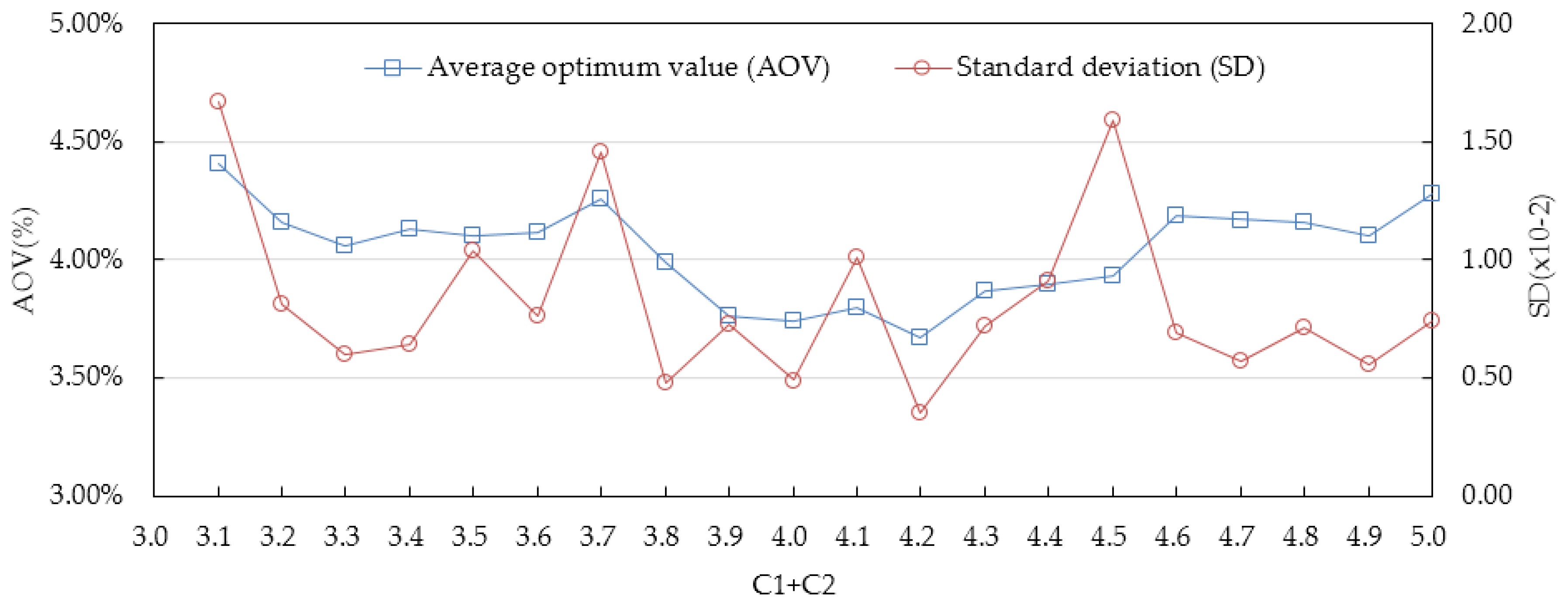
3.4. Parameters Identification by Improved Particle Swarm Optimization (PSO)

As mentioned in Section 2.1, model parameters to be identified are b i , i { 2 , 3 , , N } and a . Under given input data including the characteristic sequence and factor sequences, the goal is to seek a vector of these parameters, which provides the best forecasting results. The optimal model can be formulated as follows:
min   f ( b i , a ) = M A P E = 1 n + 1 k = 1 n + 1 | x 1 ( 0 ) ( k ) x ^ 1 ( 0 ) ( k ) x 1 ( 0 ) ( k ) | × 100 % subject   to b i ( , + ) ,   i { 2 , 3 , , N } a ( , + )
where n + 1 is the data length of the characteristic sequence (containing the forecasting point).
Particle swarm optimization (PSO) is an evolutionary algorithm introduced by Kennedy and Eberhart in 1995 [46]. Due to its simplicity of implementation and ability to quickly converge to a reasonably good solution, PSO has been very widely used in many fields. However, for multimodal functions or high-dimensional problems, the canonical PSO tends to be trapped in premature convergence and provides a poor solution. Therefore, a PSO based on time-varying parameters is used in this paper to identify parameters for the proposed interval GM(0, N) model. It has been proven that the time-varying PSO can significantly improve algorithm performance in terms of the global search ability and the convergence speed [47,48,49,50]. The procedure of time-varying PSO is described in detail as follows.
Step 1. Initialize particles. The number of particles is set to 60 after repeated testing. The position vector of the t -th particle is defined as X t = { x t 1 , x t 2 , , x t N } and the velocity vector as V t = { v t 1 , v t 2 , , v t N } , where t = 1 , 2 , 3 , , 60 . The positions of particles correspond to the solution of b i , i { 2 , 3 , , N } and a . For faster convergence, the initial particles are constructed with the assistance of the multiple linear regression (MLR) model. The MLR model takes the form:
y = β X + ε
where y , X are respectively the AGO characteristic sequence X 1 ( 1 ) and factor sequences X i ( 1 ) , i = { 2 , 3 , , N } . Suppose the solution is X i n i = { β , ε } = { x 1 i n i , x 2 i n i , , x N i n i } , then:
x t d = x d i n i + r ( x m a x x m i n ) + x m i n , t = 1 , 2 , 3 , , 60 , d = 1 , 2 , 3 , , D
where x m a x = MAX 1 d N { | x d i n i | } , x m i n = MAX 1 d N { | x d i n i | } , r is a random number in interval [0, 1], d is the index of parameters and D is the dimension of particle, D = N .
Step 2. Evaluate fitness for each particle and further identify the best position (defined as P t k = { p t 1 k , p t 2 k , , p t D k } ) of each particle and the best position (defined as P g k = { p g 1 k , p g 2 k , , p g D k } ) of the swarm. Up to the k -th evolution generation, let p t b e s t denote the best fitness of the t -th particle. For each particle, if its current fitness value is better than p t b e s t , then set this value as p t b e s t and its position as P t k . Similarly, the particle with the best fitness of the swarm is identified, and its position is defined as P g k .
Step 3. Update the position and velocity for each particle, shown in Equation (25).
{ v t d k + 1 = ω v t d k + c 1 r 1 ( p t d k x t d k ) + c 2 r 2 ( p g d k x t d k ) x t d k + 1 = x t d k + v t d k + 1
where ω is the inertia weight; d = 1 , 2 , 3 , , D ; t = 1 , 2 , 3 , , 60 ; k is the current evolution generation; c 1 , c 2 are two acceleration coefficients in which c 1 is named the cognitive learning rate and c 2 is named the social learning rate; r 1 , r 2 are two random numbers in the interval [0, 1].
ω , c 1 and c 2 are three main parameters in PSO, which can significantly affect the performance of PSO. It has been demonstrated that a relatively larger value of ω is beneficial for global search, and a smaller one is good for local search [51]. Therefore, Shi [47] introduced a linear decreasing inertia weight, and later, Chatterjee [48] developed the trajectory of ω according to a nonlinear function, which is also used in this article, shown in Equation (26).
ω = ω s t a r t ( ω s t a r t ω e n d ) ( g G m a x ) 2
where ω s t a r t and ω e n d are the initial value and end value, respectively. g and G m a x represent the present and maximum evolution generation, respectively. Generally, ω s t a r t = 0.9 , ω e n d = 0.4 . G m a x is set as constant 500 in this paper. In addition, Eberhart [46] described that a relatively high cognitive learning rate c 1 is beneficial for particles to wander through the entire search space, and a large social learning rate c 2 performs better in local search. Therefore, Ratnaweera [49] and Wang [50] proposed time-varying acceleration coefficients, which can be mathematically represented as follows:
c 1 = c 1 , m a x + ( c 1 , m i n c 1 , m a x ) ( g G m a x )
c 2 = c 2 , m i n + ( c 2 , m a x c 2 , m i n ) ( g G m a x )
where, c 1 , m i n , c 1 , m a x , c 2 , m i n and c 2 , m a x are constant factors. To find out the best ranges of c 1 and c 2 , series numerical simulations are also carried out (detailed in Section 5.1).
Step 4. Repeat Steps 2–4 until the iteration reaches its maximum value. Therefore, the best fitness value can be confirmed, and its corresponding particle is obtained. The position of this particle is the optimal solution for parameters b i and a .

3.5. Summary of Calculation Process

As described above, the calculation process of our proposed interval GM(0, N) model can be summarized as below in Figure 2.

4. Study Area and Influence Factors

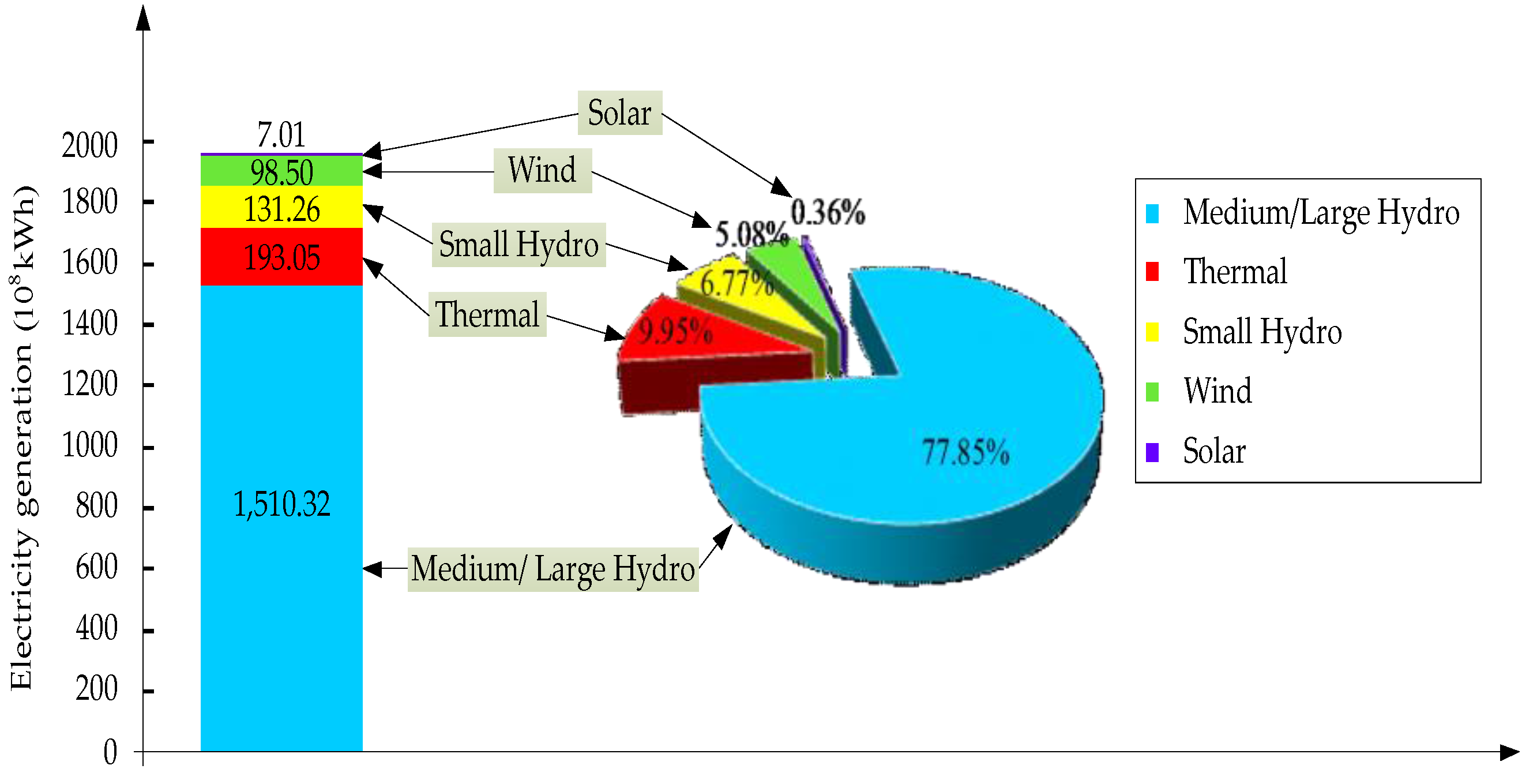
4.1. Newly-Reformed Yunnan Electricity Market

The Chinese government is starting its implementation of further electricity market reform in several piloting provinces, and Yunnan province is one of them [52]. The insufficient electricity demand and great surplus of clean energy are the main reasons for Yunnan to promote the reform of its electricity sector. At the early stage of electricity market reform, to guarantee the stability and security operation of the power grid, some units are treated as “must run units”, which do not participate in the market competition. Meanwhile, to meet the requirements of environmental policies, electricity generated by clean and renewable energy sources should be fully acquired in a competitive market, such as wind, solar and small hydro. The generation contracts are made in monthly electricity market. The process and key times of Yunnan’s monthly electricity market are shown in Figure 3. At the closure of bidding, the Yunnan Power Exchange Center (YPEC) aggregates the submitted seller and buyer bids. Then, the market supply and demand curves are generated, and the electricity MCP is calculated.

4.2. Identification of Input Variables

The biggest difference between electricity and other commodities is that it cannot be stored in large quantities, which leads to a high volatility of electricity price. Many factors may determine or affect electricity price, such as historical price, historical/forecasted load, weather conditions, macroeconomic policies, competitors’ irrational behaviors, and so on [5,10,53]. Till now, there are no consensus factors for price forecasting. Generally, the researchers tend to utilize past experience, also taking into consideration the unique economic environments of different markets, in selecting the input variables for their respective models. Therefore, we need to understand Yunnan’s supply and demand conditions and select appropriate input variables. In this paper, factors that cannot be quantified and expressed in numerical values are not considered, such as macroeconomic policies and competitors’ irrational behaviors.
Yunnan has extremely rich hydropower resources, and three of the 13 hydropower bases in China are located here. About 74.2% of the total installed capacity is hydropower, with 14.0% of small hydropower and 60.2% of medium/large hydropower. Besides hydropower, thermal, wind and solar power are also included, accounting for 16.2%, 8.0% and 1.5% of the total installed capacity respectively. Over 77% of the yearly generation in Yunnan is medium/large hydropower based; around 10% is generated by thermal power; and the remaining 13% is a mixture of production types including small hydro, wind and solar power. By the end of 2015, Yunnan’s installed capacity and electricity generation of each energy resource are shown in Figure 4 and Figure 5. Yunnan is also an important electricity supplier for China’s west-to-east electricity transmission project, Laos and Vietnam. In 2015, about 44% of the total energy production has been exported. Therefore, its electricity demand can be classified into two types: one is provincial electricity demand, and the other is export electricity demand.
Based on the experience, electricity supply and demand conditions of the Yunnan market, three types of influence factors are considered.

4.2.1. Supply Factors

The medium/large hydropower and thermal power are the main energy sources of Yunnan, which would directly affect the electricity MCP. As clean and renewable energy sources, the wind power, small hydropower and solar power all have the priority right to be purchased, which would increase the competition between other generators without the priority right and affect the electricity MCP, as well. Therefore, the available energy of each energy resource is concerned, and the energy production is considered as the input variable on the supply factors’ side. It is noted that the factors that can further influence energy production are not included. The reasons for this are: (1) compared with energy production, the factors that can influence energy production are having relatively indirect influences on the market price; to a certain degree, their influences on the market price have already been reflected in that of energy production; and (2) the factors that influence energy production can be various, and some of them are unavailable. Take hydropower as an example: its energy production is strongly correlated with runoffs, reservoir’s capacity and level, unit maintenance, flood prevention requirements, operation rules, and so on. It seems extremely difficult to consider all of these factors; the adopted energy production is a synthetic effect of these on electricity MCP. Besides, the portion that does not participate in the market competition (such as must run units) has been excluded from the available energies.

4.2.2. Demand Factors

The electricity MCP is obviously related to the market demand. Currently, in Yunnan, more than 40% of generated electricity is transmitted to outside areas through mid- or long-term contracts. The amount of export electricity has an influence on the competition of provincial electricity consumers and should affect the electricity MCP. For the provincial electricity demand, about 90% is provided in the monthly electricity market. The export electricity demand and provincial electricity demand are the main demand factors and selected as input variables.

4.2.3. Supplemented Factors

In Yunnan’s developing electricity market, there are only two types of participants so far: the generating companies (GENCOs) and consumption companies (CONCOs). The number of GENCOs and CONCOs reflects the competition in the supply and demand sides. With more market participants, the market tends to be a perfectly competitive market, and the electricity MCP changes. Here, the number of GENCOs and CONCOs in the electricity market is used as supplemented input variables.
The input variables for electricity MCP forecasting considered in this article are listed in the following Table 2. Meanwhile, we should notice that the selection of appropriate input variables plays an important role in ensuring accuracy. For different electricity markets, the energy source compositions and economic environments are obviously different, resulting in specific input variables. The proposed model is promising to be applied to other electricity markets, but the input variables should be carefully re-identified before modeling.

4.3. Data Collection and Normalization

For the case study, actual monthly data including MCP sequence and factor sequences in the Yunnan electricity market, from April 2015–April 2016 are used. The data shown in Table 3 are normalized by the min-max normalization ( N o r . ), which is formulated as:
X = X X m i n X m a x X m i n
where X m a x and X m i n are the maximum and minimum values of the X sequence, respectively. Correspondingly, the inverse normalization transformation ( I n v . ) is:
X = X ( X m a x X m i n ) + X m i n

5. Case Study

5.1. An Example for Forecasting

To detail the forecasting procedure of the proposed interval GM(0, N) model, a forecasting example for April 2016 is given. In this case study, the proposed model is trained by data from April 2015–March 2016. The procedure is described as follows.
Step 1. According to Section 3.1, the influence factor F 1 is selected as the benchmark ranking sequence because it has nearly the reverse ranking order and the highest correlation coefficient with the MCP sequence. The correlation coefficient is 0.9059. Then, all data sequences that contain the forecasting point are ranked in accordance with the descending order of F 1 , partly shown in Table 4.
Step 2. The position of forecasting point is determined by comparing the F 1 value of April 2016 with other months, i.e., between December 2015 and March 2016. Two neighboring values, respectively 0.7791 and 0.4726, are used as two virtual values for April 2016. Thus, the upper- and lower-bound MCP sequences are constructed. They are:
X 1 u p ( 0 ) = { 0.0000 , 0.0105 , , 0.4726 , 0.7791 , 0.7791 , , 1.0000 }
X 1 l o w ( 0 ) = { 0.0000 , 0.0105 , , 0.4726 , 0.4726 , 0.7791 , , 1.0000 }
Step 3. Two improved GM(0, N) models are respectively built from the upper- and lower-bound MCP sequences combined with ranked factor sequences. Additionally, the model parameters are identified by the time-varying PSO as described in Section 3.4. To find out the best ranges of c 1 and c 2 , numerical simulations are carried out. Based on the values used in [49,50,54,55,56,57,58], the test range of c 1 + c 2 is set to [3.0, 5.0]. The average and standard deviation of the optimum solutions for 100 trials of different values of c 1 + c 2 are shown in Table 5, and curves are presented in Figure 6 accordingly. From the result, we can see that when c 1 + c 2 = 4.2 , the performance is best. Thus, in our study, with the increasing of iterations, c 1 is decreasing from 3.7 down to 0.5, and c 2 is increasing from 0.5–3.7. In this way, the resulting MCP forecasting interval is [0.4787, 0.7910]. The evolution process of best fitness when calculating upper- and lower-bound forecasting values by the time-varying PSO is shown below in Figure 7.
Step 4. As described in Section 3.3, the proportion coefficient α is calculated by Equation (21). Thus, the definite forecasting value of April 2016 is:
x ^ 1 ( 0 ) = α x ^ 1 l o w ( 0 ) + ( 1 α ) x ^ 1 u p ( 0 ) = 0.4700 × 0.4787 + ( 1 0.4700 ) × 0.7910 = 0.6442
Therefore, the forecasting value of April 2016 is 0.2803 after inverse normalization transformation. As the observed value is 0.2893, the MAE and MAPE are respectively | 0.2893 0.2803 | = 0.0090 and | 0.2893 0.2803 | ÷ 0.2893 × 100 % = 3.10 % . The forecasting result is acceptable. It is important to note that the forecasting result is based on the assumption that the input factor sequences of the forecasting point are accurately predicted.

5.2. Sensitivity Analysis of Position

To validate the applicability of the proposed interval GM(0, N) model, a sensitivity analysis of the position of the forecasting point is discussed. Here, also take the MCP forecasting of April 2016 as an example. The true position of April 2016 in the ranked MCP sequence is Position 1. Suppose that the position is somehow misjudged; define the left position as Position 2 and the right as Position 3, as shown in Figure 8.
The proposed interval GM(0, N) model is applied to three different positions respectively, and the results are shown in Table 6. The MAPE for Position 1 is 3.10%, which is the best among the three positions. It obviously shows that the correct position estimation can provide a more accurate forecasting interval, which has a direct influence on the forecasting result. For Positions 2 and 3, the MAPEs are 8.28% and 4.79%, respectively. Compared to Position 1, although their forecasting performances are deteriorating, they are also acceptable in mid-term forecasting. The MAPE of the three positions is 5.39%. By taking into account the correlation between electricity MCP and influence factors, the coefficient α given by the developed novel whitenization method has a certain degree of correction to the forecasting interval. As shown in Figure 9, whether the position of the forecasting point is correct or not, the coefficient α will guide the forecasting interval towards the actual value, which also shows a better result than the equal proportion method ( α = 0.5 ). For Positions 1 and 2, the forecasting interval is on the left of the observed value, so the direction of α is from left to right. On the other hand, the forecasting interval of Position 3 is on the right; the direction is accordingly from right to left. Although the position of the forecasting point is not exactly judged in some cases, if the deviation of the position is not too big, the proposed model can obtain an acceptable forecasting result.

5.3. Comparison with Other Models

To further illustrate the forecasting performance of the proposed interval GM(0, N) model (Model 4), three other forecasting models are established for comparison, i.e., the multiple linear regression (MLR) model (Model 1), the traditional GM(0, N) model (Model 2) and the artificial neural network (ANN) model (Model 3). The MLR model is a typical static model for price forecasting by investigating the relationship between a dependent variable and several independent variables, which is also shaped like the proposed model. The used ANN model is a typical three-layered back propagation neural network model, including one input layer, one hidden layer and one output layer, which is usually preferred in practical engineering applications [23,59,60]. The sigmoid transfer function is used in both the neurons of the hidden and output layers. Nine inputs (influence factors) and one output (market price) are applied to the ANN model. At the training stage, the Levenberg–Marquardt algorithm is used to train the ANN model. Various numbers of neurons in the hidden layer are tested, and all statistical criteria of these network structures are recorded and compared. The best results are produced with 11 hidden units. The maximum iterations used in this paper is 1000. All four models are applied to forecast electricity MCP for each month in turn from April 2015–April 2016 under the same experimental conditions. For each month, the data of other months are used as input data for building these models respectively.
Forecasting results of these models are shown in Table 7 and Figure 10. We can see that the proposed interval GM(0, N) model shows a higher precision than the other compared models. The MAPE of the proposed model is 3.80%, and that of the MLR model is 22.06%; the traditional GM(0, N) model is 23.70%; the ANN model is 8.00%. Although the MAPE of the ANN model does not differ very greatly from that of the proposed model, the fluctuation of its results is much higher. The maximum absolute percentage error of the ANN model is 21.12%, which is not acceptable. The error variance of the proposed model is 0.0297, which is also much less than the MLR model (0.1581), the traditional GM(0, N) model (0.1801) and the ANN model (0.0550). For fitting precision checking, the C and P of the proposed model are 0.32 and 100.0%, respectively, showing a good fitting precision grade. While these of the traditional GM(0, N) model are 2.22 and 30.78%, respectively, the forecasting result is unqualified. This truly shows that our improvements on the traditional GM(0, N) model are effective in mid-term electricity MCP forecasting, and good forecasting results are obtained.

5.4. Forecasting Evaluation Based on the Modified Diebold–Mariano (MDM) Test

In this part, the forecasting performance is compared via the MDM test. The MDM test is carried out respectively between our proposed model and the other three forecasting models. The evaluation results are summarized in Table 8.
From Table 8, conclusions can be drawn by comparison of Model 1 and Model 4:
  • According to the MDM test based on the MAE loss function, the null hypothesis is rejected at the 1% level of significance. In other words, the observed differences are pretty significant, and the forecasting performance of Model 4 is better than Model 1.
  • According to the MDM test based on the MSE loss function, the null hypothesis is rejected at the 10% level of significance. That is to say, the observed differences are also significant, and the forecasting performance of Model 4 is better than Model 1.
Similarly, according to the comparisons of Models 2 and 4 and Models 3 and 4, both the MDM test by MAE and MSE loss functions evaluate that the forecasting performance of Model 4 is better than Models 2 and 3. Therefore, the superiority of the proposed model is further validated statistically.

6. Conclusions

Accurate mid-term electricity MCP forecasting is essential for all market participants. In this paper, a novel interval GM(0, N) model for mid-term electricity MCP forecasting is proposed, aiming to present a feasible method for the electricity market with few available data. In the proposed model, two improved GM(0, N) models are included to respectively estimate the upper- and lower-bound forecasting values. Firstly, all input sequences (not containing further values) including the MCP sequence and factor sequences are ranked in accordance with the ascending order of the MCP sequence. Then, one of the factor sequences is selected as the benchmark ranking sequence according to its ranking order and correlation with the MCP sequence. The position of forecasting point in the MCP sequence thus can be determined by the benchmark ranking sequence. Finally, the upper and lower points of the forecasting point in the MCP sequence are regarded as two virtual values to construct two new MCP sequences, which are respectively used as input for two improved GM(0, N) models, obtaining the forecasting interval. In the two improved GM(0, N) models, the input sequences used for modeling include not only known data, but also the virtual MCP and predicted factors of the forecasting point, and model parameters are identified by an improved PSO instead of LSM. Based on the forecasting interval, a novel whitenization method, taking correlation coefficient weighted gaps of factor sequences into consideration, is also established to determine the definite forecasting value.
The proposed model has been applied to the newly-reformed Yunnan electricity market. Being at the early stage of reform, this market shares many common features with restructuring practices in other countries, while simultaneously exhibiting many unique characteristics, as well. After careful analysis of its market conditions, the input variables are appropriately determined, among which the energy production of medium/large hydro power is selected as the benchmark ranking sequence. For April 2016, the absolute percentage error of the forecasting value is 3.10%. Additionally, the MAPE of the proposed model for MCP forecasting from April 2015–April 2016 is 3.80%, which shows a better forecasting performance compared with the MLR model, the traditional GM(0, N) model and the ANN model, and its superiority is also confirmed by the modified Diebold–Mariano test. The good forecasting results indicate that the proposed model is suitable for mid-term electricity MCP forecasting in a data-sparse electricity market.

Acknowledgments

This study is supported by the National Natural Science Foundation of China (No. 91547201) and the Major International Joint Research Project from the National Nature Science Foundation of China (51210014).

Author Contributions

Chuntian Cheng and Bin Luo developed and solved the proposed model and carried out this analysis. Bin Luo, Shumin Miao and Xinyu Wu wrote the manuscript and contributed to the revisions.

Conflicts of Interest

The authors declare no conflict of interest.

References

  1. The Communist Party of China (CPC) Central Committee and State Council of PRC. Opinions on Further Deepening the Reforms of electricity power system. Available online: http://www.cec.org.cn/huanbao/xingyexinxi/fazhangaige/2015-03-25/135625.html (accessed on 25 March 2015).
  2. Ma, C.; He, L. From state monopoly to renewable portfolio: Restructuring China’s electric utility. Energy Policy 2008, 36, 1697–1711. [Google Scholar] [CrossRef]
  3. Yan, X.; Chowdhury, N.A. Mid-term electricity market clearing price forecasting: A hybrid LSSVM and ARMAX approach. Int. J. Electr. Power Energy Syst. 2013, 53, 20–26. [Google Scholar] [CrossRef]
  4. Weron, R. Electricity price forecasting: A review of the state-of-the-art with a look into the future. Int. J. Forecast. 2014, 30, 1030–1081. [Google Scholar] [CrossRef]
  5. Aggarwal, S.K.; Saini, L.M.; Kumar, A. Electricity price forecasting in deregulated markets: A review and evaluation. Int. J. Electr. Power Energy Syst. 2009, 31, 13–22. [Google Scholar] [CrossRef]
  6. Rubin, O.D.; Babcock, B.A. The impact of expansion of wind power capacity and pricing methods on the efficiency of deregulated electricity markets. Energy 2013, 59, 676–688. [Google Scholar] [CrossRef]
  7. Sapio, S.; Wylomanska, A. The impact of forward trading on the spot power price volatility with Cournot competition. In Proceedings of the 5th international conference on the European electricity market, Lisboa, Portugal, 28–30 May 2008; pp. 105–110.
  8. Ruibal, C.M.; Mazumdar, M. Forecasting the mean and the variance of electricity prices in deregulated markets. IEEE Trans. Power Syst. 2008, 23, 25–32. [Google Scholar] [CrossRef]
  9. Wood, A.J.; Wollenberg, B.F. Power Generation, Operation and Control; Wiley: New York, NY, USA, 1996. [Google Scholar]
  10. Batlle, C.; Barquin, J. A strategic production costing model for electricity market price analysis. IEEE Trans. Power Syst. 2005, 20, 67–74. [Google Scholar] [CrossRef]
  11. Kian, A.; Keyhani, A. Stochastic price modeling of electricity in deregulated energy markets. In Proceedings of the 34th Annual Hawaii International Conference on System Sciences, Maui, HI, USA, 6 January 2001; pp. 1–7.
  12. Robinson, T.A. Electricity pool prices: A case study in nonlinear time-series modelling. Appl. Econ. 2000, 32, 527–532. [Google Scholar] [CrossRef]
  13. Carpio, J.; Juan, J.; López, D. Multivariate exponential smoothing and dynamic factor model applied to hourly electricity price analysis. Technometrics 2014, 56, 494–503. [Google Scholar] [CrossRef]
  14. Nogales, F.J.; Contreras, J.; Conejo, A.J.; Espinola, R. Forecasting next-day electricity prices by time series models. IEEE Trans. Power Syst. 2002, 17, 342–348. [Google Scholar] [CrossRef]
  15. Obradovic, Z.; Tomsovic, K. Time series methods for forecasting electricity market pricing. In Proceedings of the IEEE Power Engineering Society Summer Meeting, Edmonton, AB, Canada, 18–22 July 1999; pp. 1264–1265.
  16. Cuaresma, J.C.; Hlouskova, J.; Kossmeier, S.; Obersteiner, M. Forecasting electricity spot-prices using linear univariate time-series models. Appl. Energy 2004, 77, 87–106. [Google Scholar] [CrossRef]
  17. Conejo, A.J.; Plazas, M.A.; Espinola, R.; Molina, A.B. Day-ahead electricity price forecasting using the Wavelet Transform and ARIMA Models. IEEE Trans. Power Syst. 2005, 20, 1035–1042. [Google Scholar] [CrossRef]
  18. Kim, C.; Yu, I.K.; Song, Y.H. Prediction of system marginal price of electricity using wavelet transform analysis. Energy Convers. Manag. 2002, 43, 1839–1851. [Google Scholar] [CrossRef]
  19. Zhang, J.; Tan, Z. Day-ahead electricity price forecasting using WT, CLSSVM and EGARCH model. Int. J. Electr. Power Energy Syst. 2013, 45, 362–368. [Google Scholar] [CrossRef]
  20. Contreras, J.; Espinola, R.; Nogales, F.J.; Conejo, A.J. ARIMA models to predict next-day electricity prices. IEEE Trans. Power Syst. 2003, 18, 1014–1020. [Google Scholar] [CrossRef]
  21. Jakaša, T.; Andročec, I.; Sprčić, P. Electricity price forecasting - ARIMA model approach. In Proceedings of the 8th International Conference on the European Energy Market (EEM), Zagreb, Croatia, 25–27 May 2011; pp. 222–225.
  22. Xie, M.; Sandels, C.; Zhu, K. A seasonal ARIMA model with exogenous variables for elspot electricity prices in Sweden. In Proceedings of the 10th International Conference on the European Energy Market (EEM), Stockholm, Sweden, 27–31 May 2013; pp. 1–4.
  23. Szkuta, B.R.; Sanabria, L.A.; Dillon, T.S. Electricity price short-term forecasting using artificial neural networks. IEEE. Trans. Power Syst. 1999, 14, 851–857. [Google Scholar] [CrossRef]
  24. Keles, D.; Scelle, J.; Paraschiv, F.; Fichtner, W. Extended forecast methods for day-ahead electricity spot prices applying artificial neural networks. Appl. Energy 2016, 162, 218–230. [Google Scholar] [CrossRef]
  25. Shrivastava, N.A.; Khosravi, A.; Panigrahi, B.K. Prediction interval estimation of electricity prices using PSO-Tuned Support Vector Machines. IEEE Trans. Ind. Inf. 2015, 11, 322–331. [Google Scholar] [CrossRef]
  26. Papadimitriou, T.; Gogas, P.; Stathakis, E. Forecasting energy markets using support vector machines. Energy Econ. 2014, 44, 135–142. [Google Scholar] [CrossRef]
  27. Zhao, J.H.; Dong, Z.; Li, X.; Wong, K. A framework for electricity price spike analysis with advanced data mining methods. IEEE Trans. Power Syst. 2007, 22, 376–385. [Google Scholar] [CrossRef]
  28. Huang, D.; Zareipour, H.; Rosehartet, W.D.; Amjady, N. Data mining for electricity price classification and the application to demand-side management. IEEE Trans. Smart Grid 2012, 3, 808–817. [Google Scholar] [CrossRef]
  29. Tan, Z.F.; Zhang, J.L.; Wang, J.H.; Xu, J. Day-ahead electricity price forecasting using wavelet transform combined with ARIMA and GARCH models. Appl. Energy 2010, 87, 3606–3610. [Google Scholar] [CrossRef]
  30. Gonzalez, V.; Contreras, J.; Bunn, D. Forecasting power prices using a hybrid Fundamental-Econometric model. IEEE Trans. Power Syst. 2012, 27, 363–372. [Google Scholar] [CrossRef]
  31. Cerjan, M.; Matijaš, M.; Delimar, M. Dynamic hybrid model for short-term electricity price forecasting. Energies 2014, 7, 3304–3318. [Google Scholar] [CrossRef]
  32. Torghaban, S.S.; Zareipour, H.; Tuan, L.A. Medium-term electricity market price forecasting: a data-driven approach. In Proceedings of the 2010 North American Power Symposium (NAPS 2010), Arlington, TX, USA, 26–28 September 2010; pp. 1–7.
  33. Torghaban, S.S.; Motamedi, A.; Zareipour, H.; Tuan, L.A. Medium-term electricity price forecasting. In Proceedings of the 2012 North American Power Symposium (NAPS 2012), Champaign, IL, USA, 9–11 September 2012; pp. 1–8.
  34. Bello, A.; Reneses, J.; Munoz, A. Medium-term probabilistic forecasting of extremely low prices in electricity markets: Application to the Spanish case. Energies 2016, 9, 193. [Google Scholar] [CrossRef]
  35. Yan, X.; Chowdhury, N.A. Mid-term electricity market clearing price forecasting: A multiple SVM approach. Int. J. Electr. Power Energy Syst. 2014, 58, 206–214. [Google Scholar] [CrossRef]
  36. Liu, S.; Forrest, J.; Yang, Y. A brief introduction to grey systems theory. Grey Systems: Theory Appl. 2012, 2, 89–104. [Google Scholar] [CrossRef]
  37. Deng, J.L. The control problem of grey systems. Syst. Control Lett. 1982, 1, 288–294. [Google Scholar]
  38. Qiu, B.J.; Zhang, J.H.; Qi, Y.T.; Liu, Y. Grey-theory-based optimization model of emergency logistics considering time uncertainty. PLoS ONE 2015, 10, e0139132. [Google Scholar] [CrossRef] [PubMed]
  39. Wei, J.C.; Zhou, L.; Wang, F.; Wu, D.S. Work safety evaluation in Mainland China using grey theory. Appl. Math. Model. 2015, 39, 924–933. [Google Scholar] [CrossRef]
  40. Zhou, H.; Wu, X.H.; Wang, W.; Chen, L.P. Forecast of next day clearing price in deregulated electricity market. In Proceedings of the IEEE International Conference on Systems, Man and Cybernetics, San Antonio, TX, USA, 11–14 October 2009; pp. 4397–4401.
  41. Lei, M.; Feng, Z. A proposed grey model for short-term electricity price forecasting in competitive power markets. Int. J. Electr. Power Energy Syst. 2012, 43, 531–538. [Google Scholar] [CrossRef]
  42. Ou, S.L. Forecasting agricultural output with an improved grey forecasting model based on the genetic algorithm. Comput. Electron. Agr. 2012, 85, 33–39. [Google Scholar] [CrossRef]
  43. Wang, C.H.; Hsu, L.C. Using genetic algorithms grey theory to forecast high technology industrial output. Appl. Math. Comput. 2008, 95, 256–263. [Google Scholar] [CrossRef]
  44. Harvey, D.; Leybourne, S.; Newbold, P. Testing the equality of prediction mean squared errors. Int. J. Forecast. 1997, 13, 281–291. [Google Scholar] [CrossRef]
  45. Diebold, F.X.; Mariano, R.S. Comparing predictive accuracy. J. Bus. Econ. Stat. 1995, 13, 253–263. [Google Scholar]
  46. Eberhart, R.; Kennedy, J. A new optimizer using particle swarm theory. In Proceedings of the 6th micro-machine and human, science, Nagoya, Japan, 4–6 October 1995; pp. 39–43.
  47. Shi, Y.; Eberhart, R. Empirical study of particle swarm optimization. In Proceedings of the IEEE International Congress, Evolutionary Computation, Washington, DC, USA, 6–9 July 1999; pp. 101–106.
  48. Chatterjee, A.; Siarry, P. Nonlinear inertia weight variation for dynamic adaptation in particle swarm optimization. Comput. Oper. Res. 2006, 33, 859–871. [Google Scholar] [CrossRef]
  49. Ratnaweera, A.; Halgamuge, S.K.; Watson, H.C. Self-organizing hierarchical particle swarm optimizer with time-varying acceleration coefficients. IEEE Trans. Evol. Comput. 2004, 8, 240–255. [Google Scholar] [CrossRef]
  50. Wang, Y.; Zhou, J.Z.; Zhou, C. An improved self-adaptive PSO technique for short-term hydrothermal scheduling. Expert Syst. Appl. 2012, 39, 2288–2295. [Google Scholar] [CrossRef]
  51. Shi, Y.; Eberhart, R. A modified particle swarm optimizer. In Proceedings of the IEEE World Congress on Computational Intelligence, Anchorage, AK, USA, 4–9 May 1998; pp. 69–73.
  52. National Development and Reform Commission. Notice to Accelerate Reform of Transmission and Distribution Price. Available online: http://jgs.ndrc.gov.cn/zcfg/201504/t20150416_688233.html (accessed on 13 April 2014).
  53. Gao, F.; Guan, X.; Cao, X.; Papalexopoulos, A. Forecasting power market clearing price and quantity using a neural network method. In Proceedings of the Power Engineering Society Summer Meeting, Seattle, WA, USA, 16–20 July 2000; pp. 2183–2188.
  54. Jiang, Y.; Liu, C.; Huang, C. Improved particle swarm algorithm for hydrological parameter optimization. Appl. Math. Comput. 2010, 217, 3207–3215. [Google Scholar] [CrossRef]
  55. Montalvo, I.; Izquierdo, J.; Pérez, R. A diversity-enriched variant of discrete PSO applied to the design of water distribution networks. Eng. Optimiz. 2008, 40, 655–668. [Google Scholar] [CrossRef]
  56. Gong, Y.J.; Zhang, J.; Chung, H.S. An efficient resource allocation scheme using particle swarm optimization. IEEE Trans. Evol. Comput. 2012, 16, 801–816. [Google Scholar] [CrossRef]
  57. Clerc, M.; Kennedy, J. The particle swarm-explosion, stability, and convergence in a multidimensional complex space. IEEE Trans. Evol. Comput. 2002, 6, 58–73. [Google Scholar] [CrossRef]
  58. Trelea, I.C. The particle swarm optimization algorithm: convergence analysis and parameter selection. Inf. Process. Lett. 2003, 85, 317–325. [Google Scholar] [CrossRef]
  59. Zhang, J.; Cheng, C.T. Day-ahead electricity price forecasting using artificial intelligence. In Proceedings the of IEEE Electric Power and Energy Conference, Vancouver, BC, Canada, 6–7 October 2008; pp. 1–5.
  60. Cheng, C.T.; Niu, W.J.; Feng, Z.K.; Shen, J.J.; Chau, K.W. Daily reservoir runoff forecasting method using artificial neural network based on quantum-behaved particle swarm optimization. Water 2015, 7, 4232–4246. [Google Scholar] [CrossRef]
Figure 1. The schematic diagram of the whitenization method.
Energies 09 00804 g001
Figure 2. Flow chart of the calculation process of the proposed interval GM(0, N) model.
Energies 09 00804 g002
Figure 3. The process and key times of Yunnan’s monthly electricity market.
Energies 09 00804 g003
Figure 4. The installed capacity mix of Yunnan at the end of 2015.
Energies 09 00804 g004
Figure 5. The electricity generation mix of Yunnan at the end of 2015.
Energies 09 00804 g005
Figure 6. The curves of the average optimum value (AOV) and standard deviation (SD) for 100 trials of different values of c 1 + c 2 .
Energies 09 00804 g006
Figure 7. The evolution process of best fitness when calculating upper- and lower-bound forecasting values.
Energies 09 00804 g007
Figure 8. Different positions of April 2016 in the ranked market clearing price (MCP) sequence.
Energies 09 00804 g008
Figure 9. Definite forecasting values of Positions 1–3 determined by the novel whitenization method.
Energies 09 00804 g009
Figure 10. Forecasting results of different models from April 2015–April 2016.
Energies 09 00804 g010
Table 1. Reference for the fitting precision grade.
ParametersFitting Precision Grade
GoodQualifiedJustUnqualified
C <0.350.35–0.500.50–0.65≥0.65
P >0.950.80–0.950.70–0.80≤0.70
Table 2. The input variables for electricity market clearing price (MCP) forecasting.
IndexTypesInput VariablesSymbols
1Supply factorsEnergy production of medium/large hydro power F 1
2Energy production of thermal power F 2
3Energy production of small hydro power F 3
4Energy production of wind power F 4
5Energy production of solar power F 5
6Demand factorsExport electricity demand F 6
7Provincial electricity demand F 7
8Supplemented factorsNumber of GENCOs F 8
9Number of CONCOs F 9
Table 3. Monthly MCP and influence factors of the Yunnan electricity market from April 2015–April 2016.
MonthMCP F 1 F 2 F 3 F 4 F 5 F 6 F 7 F 8 F 9
April 20150.91740.20150.86890.03740.33540.09450.29720.72690.34620.0044
May 20150.41280.36300.85920.02900.29250.01990.53150.73430.23080.0000
June 20150.04940.59850.35320.31250.17010.00000.69650.88760.38460.1027
July 20150.00001.00000.36470.88160.00000.09950.91560.87740.61540.1754
August 20150.01050.92980.29921.00000.02410.09951.00000.93680.50000.1789
September 20150.02960.78410.00000.88540.03770.09450.96571.00000.23080.2170
October 20150.03030.76270.71970.52640.25430.15920.89490.98850.26920.2365
November 20150.16920.36670.73060.33540.37470.29850.36930.52180.26920.2294
December 20150.47260.33811.00000.28950.47410.34830.31010.52200.00000.1798
January 20160.92590.18900.67540.13600.64100.53230.22680.84761.00000.8335
February 20161.00000.00000.43390.00000.80950.61690.00000.00000.92310.6740
March 20160.77910.20340.51400.00531.00001.00000.27830.43500.92310.7741
April 20160.73300.25470.55460.00310.65990.77610.29920.70861.00001.0000
Table 4. Ranked monthly MCP and the influence factors that contain the forecasting point.
MonthMCP F 1 F 2 F 3 F 4 F 5 F 6 F 7 F 8 F 9
------
May 20150.41280.36300.85920.02900.29250.01990.53150.73430.23080.0000
December 20150.47260.33811.00000.28950.47410.34830.31010.52200.00000.1798
April 2016 ( k ) 0.25470.55460.00310.65990.77610.29920.70861.00001.0000
March 20160.77910.20340.51400.00531.00001.00000.27830.43500.92310.7741
April 20150.91740.20150.86890.03740.33540.09450.29720.72690.34620.0044
------
Table 5. The average optimum value (AOV) and standard deviation (SD) for 100 trials of different values of c 1 + c 2 .
Different Values and Ranges of c 1 and c 2
Statistical Index c 1 + c 2 = 3.1 c 1 + c 2 = 3.2 c 1 + c 2 = 3.3 c 1 + c 2 = 3.4 c 1 + c 2 = 3.5
c 1 = 2.6~0.5 c 1 = 2.7~0.5 c 1 = 2.8~0.5 c 1 = 2.9~0.5 c 1 = 3.0~0.5
c 2 = 0.5~2.6 c 2 = 0.5~2.7 c 2 = 0.5~2.8 c 2 = 0.5~2.9 c 2 = 0.5~3.0
AOV (%)4.414.164.064.134.10
SD (×10−2)1.670.810.600.641.04
Statistical Index c 1 + c 2 = 3.6 c 1 + c 2 = 3.7 c 1 + c 2 = 3.8 c 1 + c 2 = 3.9 c 1 + c 2 = 4.0
c 1 = 3.1~0.5 c 1 = 3.2~0.5 c 1 = 3.3~0.5 c 1 = 3.4~0.5 c 1 = 3.5~0.5
c 2 = 0.5~3.1 c 2 = 0.5~3.2 c 2 = 0.5~3.3 c 2 = 0.5~3.4 c 2 = 0.5~3.5
AOV (%)4.124.263.993.763.74
SD (×10−2)0.761.460.480.730.49
Statistical Index c 1 + c 2 = 4.1 c 1 + c 2 = 4.2 c 1 + c 2 = 4.3 c 1 + c 2 = 4.4 c 1 + c 2 = 4.5
c 1 = 3.6~0.5 c 1 = 3.7~0.5 c 1 = 3.8~0.5 c 1 = 3.9~0.5 c 1 = 4.0~0.5
c 2 = 0.5~3.6 c 2 = 0.5~3.7 c 2 = 0.5~3.8 c 2 = 0.5~3.9 c 2 = 0.5~4.0
AOV (%)3.803.673.873.903.93
SD (×10−2)1.010.350.720.911.59
Statistical Index c 1 + c 2 = 4.6 c 1 + c 2 = 4.7 c 1 + c 2 = 4.8 c 1 + c 2 = 4.9 c 1 + c 2 = 5.0
c 1 = 4.1~0.5 c 1 = 4.2~0.5 c 1 = 4.3~0.5 c 1 = 4.4~0.5 c 1 = 4.5~0.5
c 2 = 0.5~4.1 c 2 = 0.5~4.2 c 2 = 0.5~4.3 c 2 = 0.5~4.4 c 2 = 0.5~4.5
AOV (%)4.194.174.164.104.28
SD (×10−2)0.690.570.710.560.74
Notes: c 1 = 2.6 ~ 0.5 means that c 1 is changing from 2.6 to 0.5, and similar to the others.
Table 6. Forecasting results of April 2016 in Positions 1–3.
PositionObserved ValueVirtual ValuesForecasting IntervalForecasting ValueMAPE (%)
Nor.Inv.LowerUpperLowerUpperαNor.Inv.
Position 10.73300.28930.47260.77910.47870.79100.47000.64420.28033.10
Position 20.41280.47260.41860.4702−0.50470.49620.26538.28
Position 30.77910.91740.77350.90982.30120.59610.27554.79
Average0.73300.28930.55480.72300.55690.72370.75550.57890.27375.39
Table 7. Forecasting results of the proposed model compared with the other three models.
MonthObserved ValueForecasting ValueAbsolute Percentage Error (%)
Model 1Model 2Model 3Model 4Model 1Model 2Model 3Model 4
April 20150.44710.33940.00000.36270.392913.0854.3210.256.58
May 20150.31070.32530.13700.28410.27782.1425.303.874.79
June 20150.21240.31010.19570.28150.192016.622.8311.753.46
July 20150.19900.10230.19010.17940.233416.811.553.425.98
August 20150.20180.24030.13690.25950.20056.6511.249.980.23
September 20150.20700.07330.32860.19490.205622.9420.852.090.25
October 20150.20720.17950.35830.22020.20334.7525.902.230.68
November 20150.24480.35300.16960.37590.311117.4312.1121.1210.68
December 20150.32680.19260.09170.35430.306919.1033.453.912.83
January 20160.44940.61141.00000.34680.498119.6266.7112.435.89
February 20160.46950.09910.33210.36010.430743.8016.2412.934.59
March 20160.40970.90140.55640.47010.412562.5818.667.680.35
April 20160.39720.17930.25020.41570.373228.1819.012.393.10
MAPE-----22.0623.708.003.80
Table 8. Forecasting evaluation results based on the modified Diebold–Mariano (MDM) test.
IndicatorsMDM Test Results between Different Models
Models 1 and 4Models 2 and 4Models 3 and 4
MDM-MAE3.2614 ***3.5409 ***3.4856 ***
MDM-MSE2.0354 *2.0850 *2.8789 **
Notes: MDM-MAE denotes the MDM test based on the MAE loss function; MDM-MSE denotes the MDM test based on the MSE loss function; ***, ** and * denote significance at the 1%, 5% and 10% levels, respectively.

