Predictive Modeling of a Paradigm Mechanical Cooling Tower: I. Adjoint Sensitivity Model

Abstract

Cooling towers discharge waste heat from an industrial process into the atmosphere, and are essential for the functioning of large energy-producing plants, including nuclear reactors. Using a numerical simulation model of the cooling tower together with measurements of outlet air relative humidity, outlet air and water temperatures enables the quantification of the rate of thermal energy dissipation removed from the respective process. The computed quantities depend on many model parameters including correlations, boundary conditions, material properties, etc. Changes in these model parameters will induce changes in the computed quantities of interest (called “model responses”). These changes are quantified by the functional derivatives (called “sensitivities”) of the model responses with respect to the model parameters. These sensitivities are computed in this work by applying the general Adjoint Sensitivity Analysis Methodology (ASAM) for nonlinear systems. These sensitivities are needed for: (i) ranking the parameters in their importance to contributing to response uncertainties; (ii) propagating the uncertainties (covariances) in these model parameters to quantify the uncertainties (covariances) in the model responses; (iii) performing predictive modeling, including assimilation of experimental measurements and calibration of model parameters to produce optimal predicted quantities (both model parameters and responses) with reduced predicted uncertainties.

1. Introduction

A mechanical draft cooling tower (MDCT) discharges waste heat from an industrial process into the atmosphere. Cooling towers are essential for the functioning of large energy-producing plants, including nuclear reactors. Using a numerical simulation model of the cooling tower together with measurements of outlet air relative humidity, outlet air and water temperatures enables the quantification of the rate of thermal energy dissipation removed from the respective process. In addition to computing the temperature drop of the cooling water as it passes through the tower, a cooling tower model that derives heat dissipation rates from thermal imagery needs to convert the remotely measured cooling tower throat or area-weighted temperature to a cooling water inlet temperature. Therefore, a cooling tower model comprises two main components, namely: (i) an inner model which computes the amount of cooling undergone by the water as it passes through the tower as a function of inlet cooling water temperature and ambient weather conditions (air temperature and humidity); and (ii) an outer model which uses a remotely measured throat or area-weighted temperature and iterates on the inlet water temperature to match the target temperature of interest. The cooling tower model produces an estimate of the rate at which energy is being discharged to the atmosphere by evaporation and sensible heat transfer. The sensible heat transfer is estimated using the computed change in air or water enthalpy as it passes through the MDCT. If the MDCT fans are on, a prescribed mass flow rate of air and water is used. If the MDCT fans are off, an additional mechanical energy equation is iteratively solved to determine the mass flow rate of air.

The flow regime in the fill section of a cooling tower, which can be cross-flow or counter-flow, determines the type of the respective cooling tower. A model for computing the steady-state thermal performance has been recently presented [1]; this model simulates both cross-flow and counter-flow wet mechanical draft cooling towers. Using as inputs the temperature and mass flow rate of the incoming water together with the temperature and humidity ratio of the incoming ambient air, this model computes the temperature and mass flow rate of the effluent water, as well as the temperature and water vapor content of the exhaust air. The air mass flow rate is specified when the cooling tower operates in the mechanical draft mode. When the fan is turned-off, the cooling tower operates in the natural draft/wind-aided mode, in which case the air mass flow rate is calculated using the numerical model.

In the present work, the counter-flow cooling tower presented in [1] is further developed by applying a considerably more accurate and efficient numerical method for computing the steady state distributions of the following quantities: (i) the water mass flow rates at the exit of each control volume along the height of the fill section of the cooling tower; (ii) the water temperatures at the exit of each control volume along the height of the fill section of the cooling tower; (iii) the air temperatures at the exit of each control volume along the height of the fill section of the cooling tower; (iv) the humidity ratios at the exit of each control volume along the height of the fill section of the cooling tower; and (v) the air relative humidity at the exit of each control volume. In contrast to many cases of non-convergence experienced by the original method [1], the numerical method applied in this work is highly efficient and yields accurate results everywhere, as shown in Section 2.1, below.

More importantly, however, this work presents the development of the adjoint cooling tower sensitivity model for computing efficiently and exactly the sensitivities (i.e., functional derivatives) of the model responses (i.e., quantities of interest) to all 52 model parameters. The adjoint sensitivity model is developed by applying the general Adjoint Sensitivity Analysis Methodology (ASAM) for nonlinear systems, which was originally presented in [2,3,4]. Even though the forward cooling tower model is nonlinear in the state functions, the adjoint sensitivity model is linear in the adjoint state functions, which correspond one-to-one to the forward state functions mentioned in the foregoing. Using the adjoint state functions, the sensitivities of each model response to all of the 52 model parameters can be computed exactly using a single adjoint model computation, as opposed to 52 computations, as would be required if the sensitivities would have been computed—approximately as opposed to exactly—using the forward model in conjunction with finite-differences. The sensitivities are needed for (i) ranking the parameters in the order of their importance for contributing to response uncertainties; (ii) propagating the uncertainties (variances and covariances) in the model parameters to quantify the uncertainties (variances and covariances) in the model responses; (iii) performing predictive modeling, which includes assimilation of experimental measurements and calibration of model parameters to produce optimally predicted nominal values for both model parameters and responses, with reduced predicted uncertainties. The development of the adjoint sensitivity model for the counter-flow cooling tower is presented in Section 2 of this work, together with results for the respective adjoint state functions. A discussion of the significance of the results obtained in this work is presented in Section 3. The predictive modeling of the counter-flow cooling tower will be performed by applying the “predictive modeling for coupled multi-physics systems” (PM_CMPS) methodology recently developed in [5]; the results of this predictive modeling will presented in the sequel to this paper [6].

2. Results

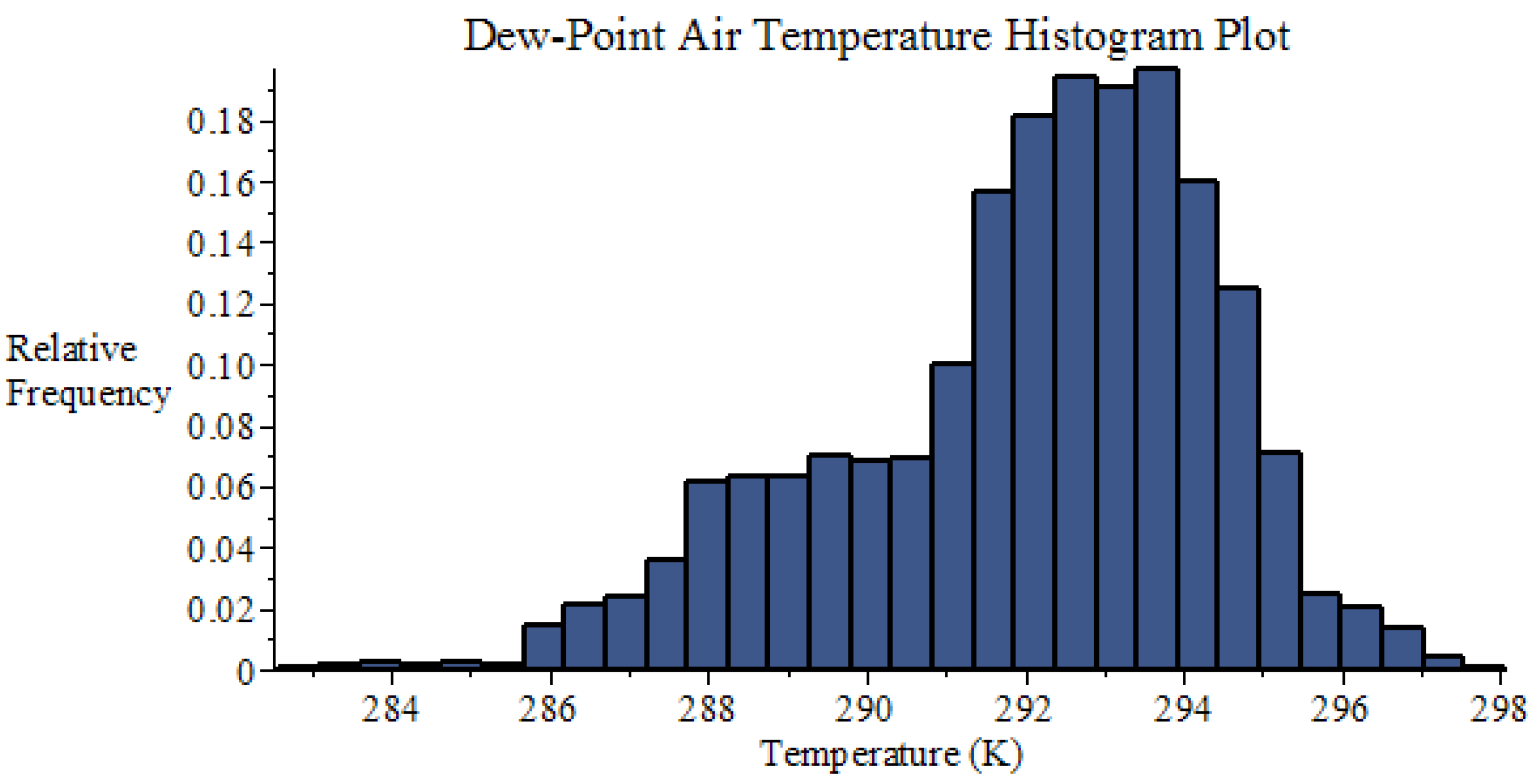
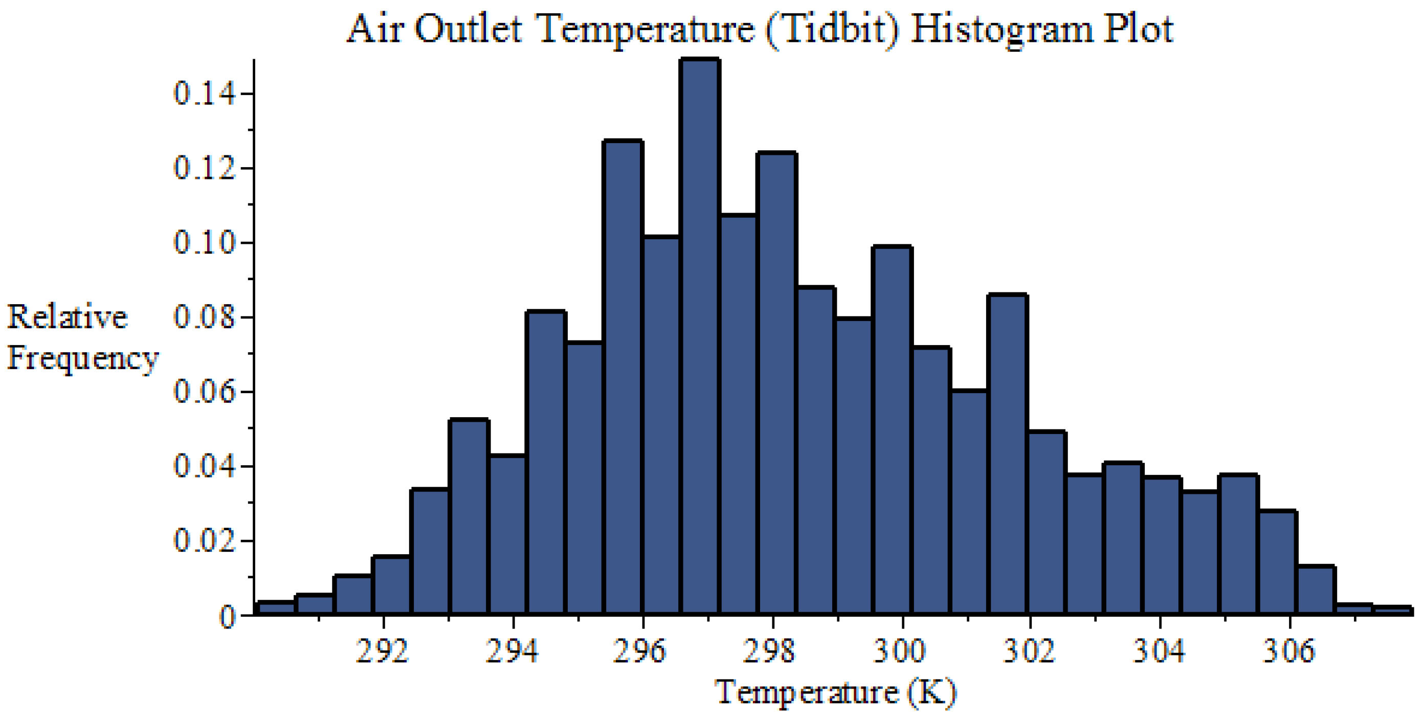
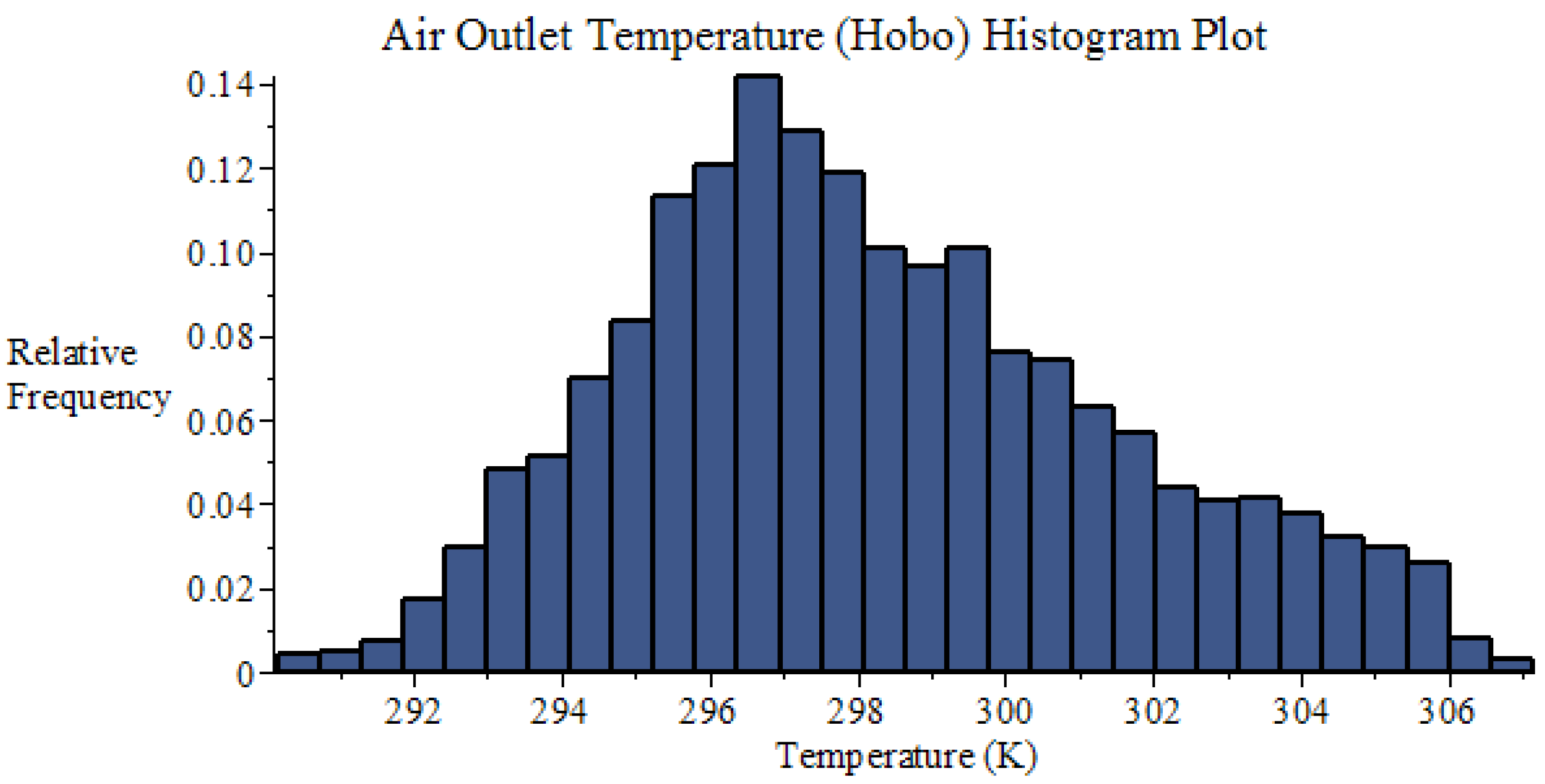
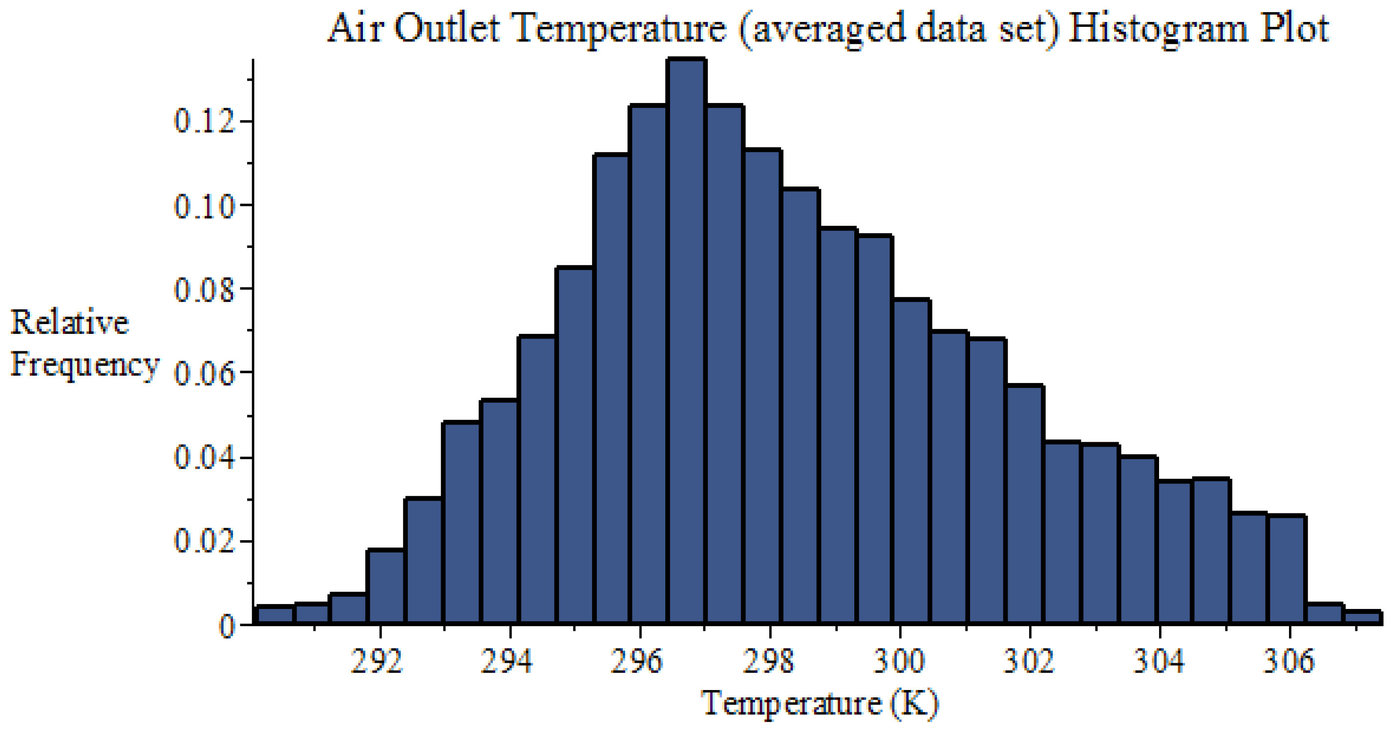
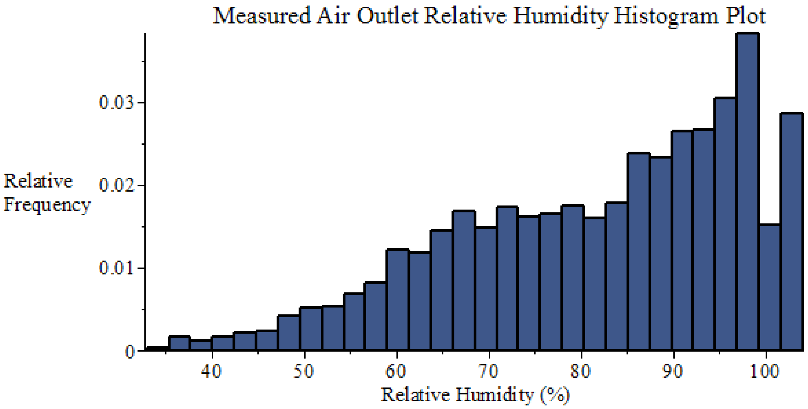
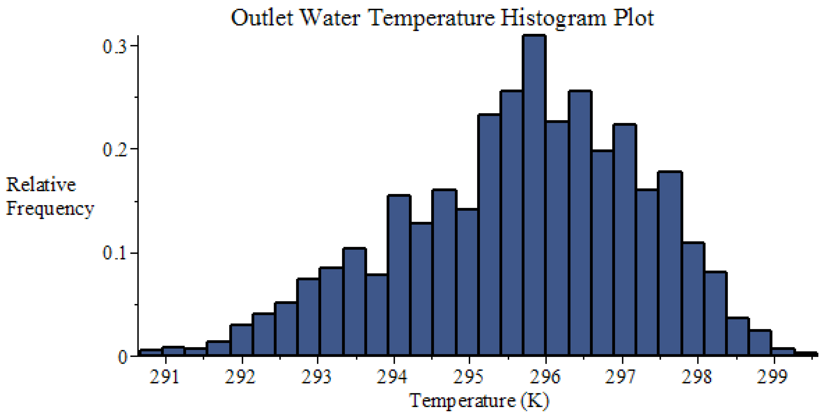
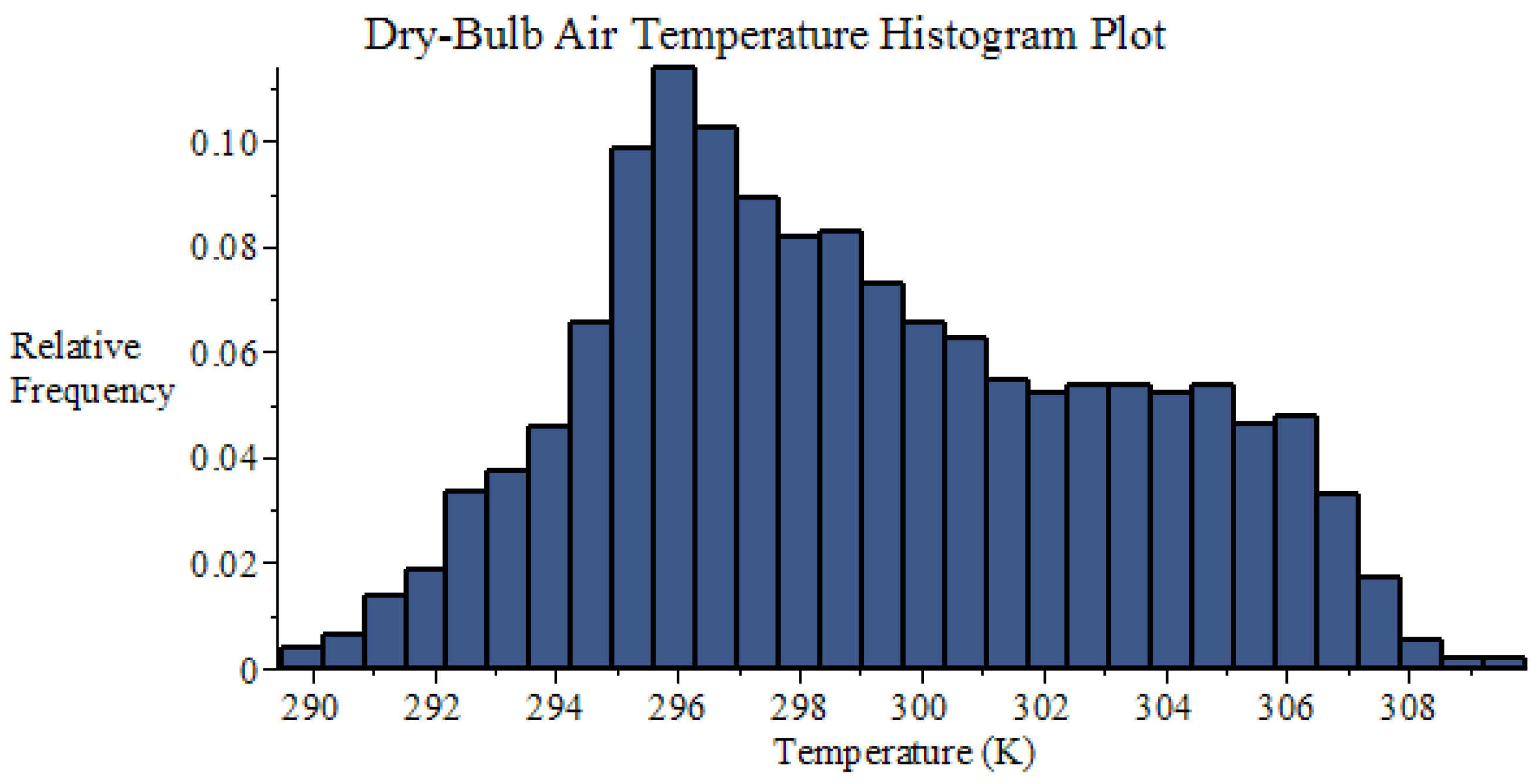
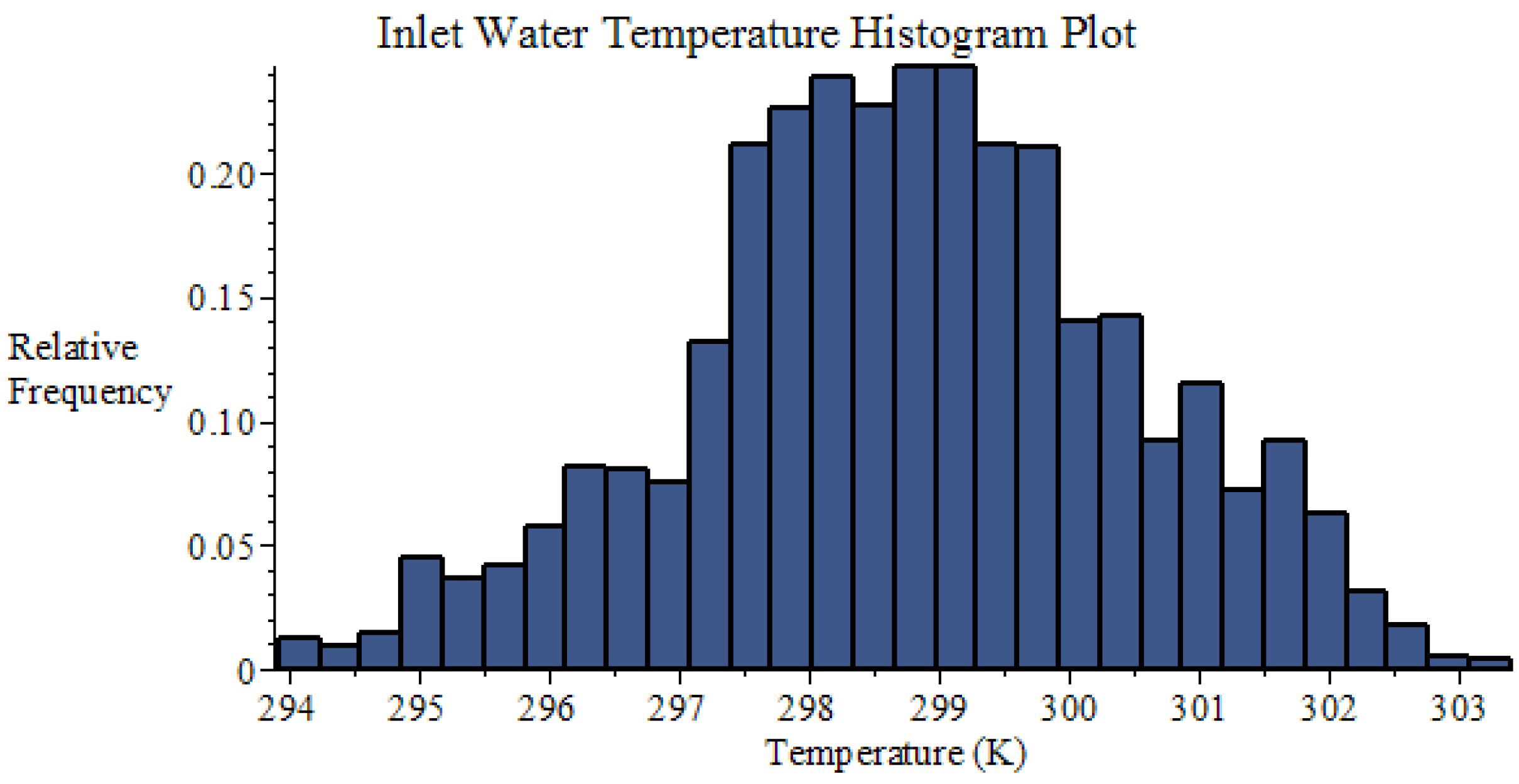
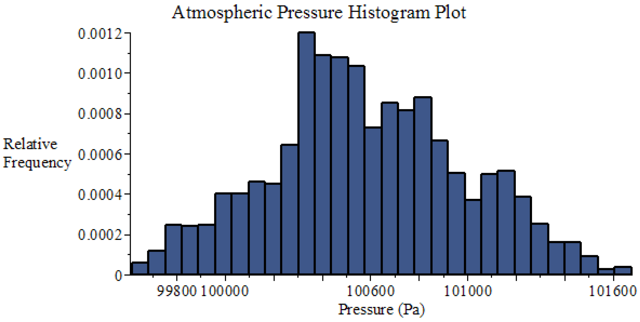
During the period from April, 2004 through August, 2004, a total 8079 measured benchmark data sets for F-area cooling towers (fan-on case) were recorded every fifteen minutes at SRNL for F-Area Cooling Towers [7]. Each of these data sets contained measurements of the following (four) quantities: (i) outlet air temperature measured with the sensor called “Tidbit”, which will be denoted as T_{a,out(Tidbit)}; (ii) outlet air temperature measured with the sensor called “Hobo”, which will be denoted as T_a,out(Hobo); (iii) outlet water temperature, which will be denoted as $T_{w,out}^{meas}$; (iv) outlet air relative humidity, which will be denoted as RH^meas. Histogram plots of these 7668 measurement sets (each set containing measurements of T_{a,out(Tidbit)}, T_a,out(Hobo), $T_{w,out}^{meas}$ and RH^meas), together with statistical analyses of these measurements, are presented in Appendix A. These measured quantities provide the basis for the choosing the state functions underlying the mathematical modeling of the cooling tower, which is presented in Section 2.1. An accurate and efficient numerical method for solving the equations underlying the counter-flow cooling tower is also presented in this section. Section 2.2 presents the development of the cooling tower adjoint sensitivity model, along with the solution method for computing the adjoint state functions. The numerical accuracy of solving the equations underlying the adjoint sensitivity model will also be verified.

2.1. Mathematical Model of the Counter-Flow Cooling Tower

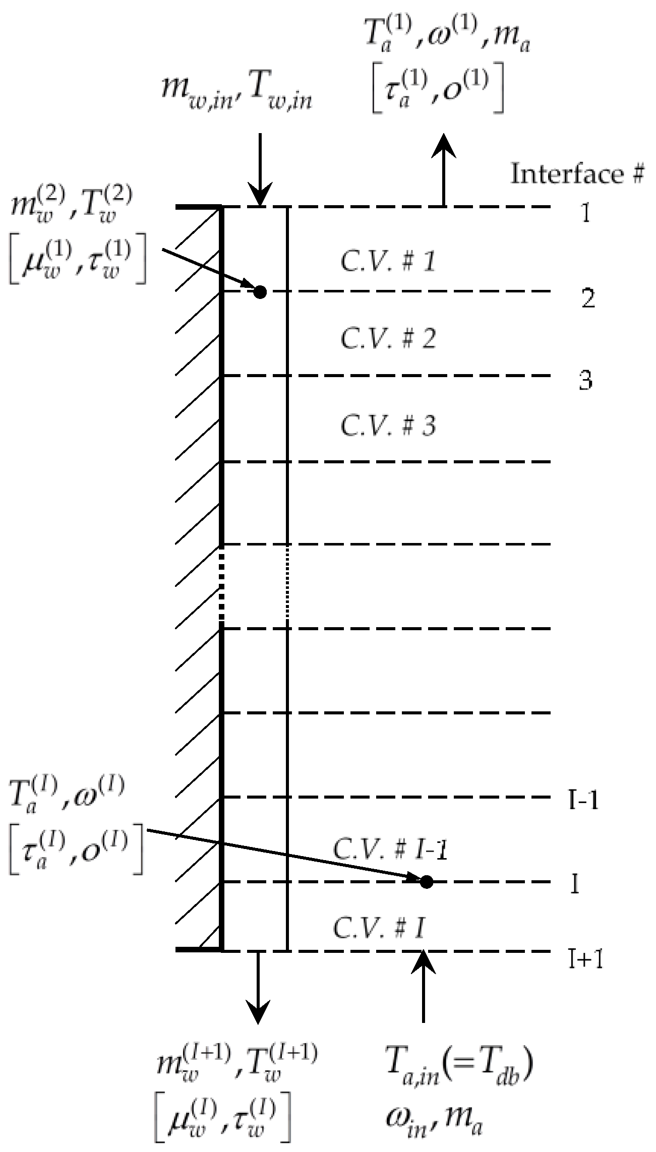
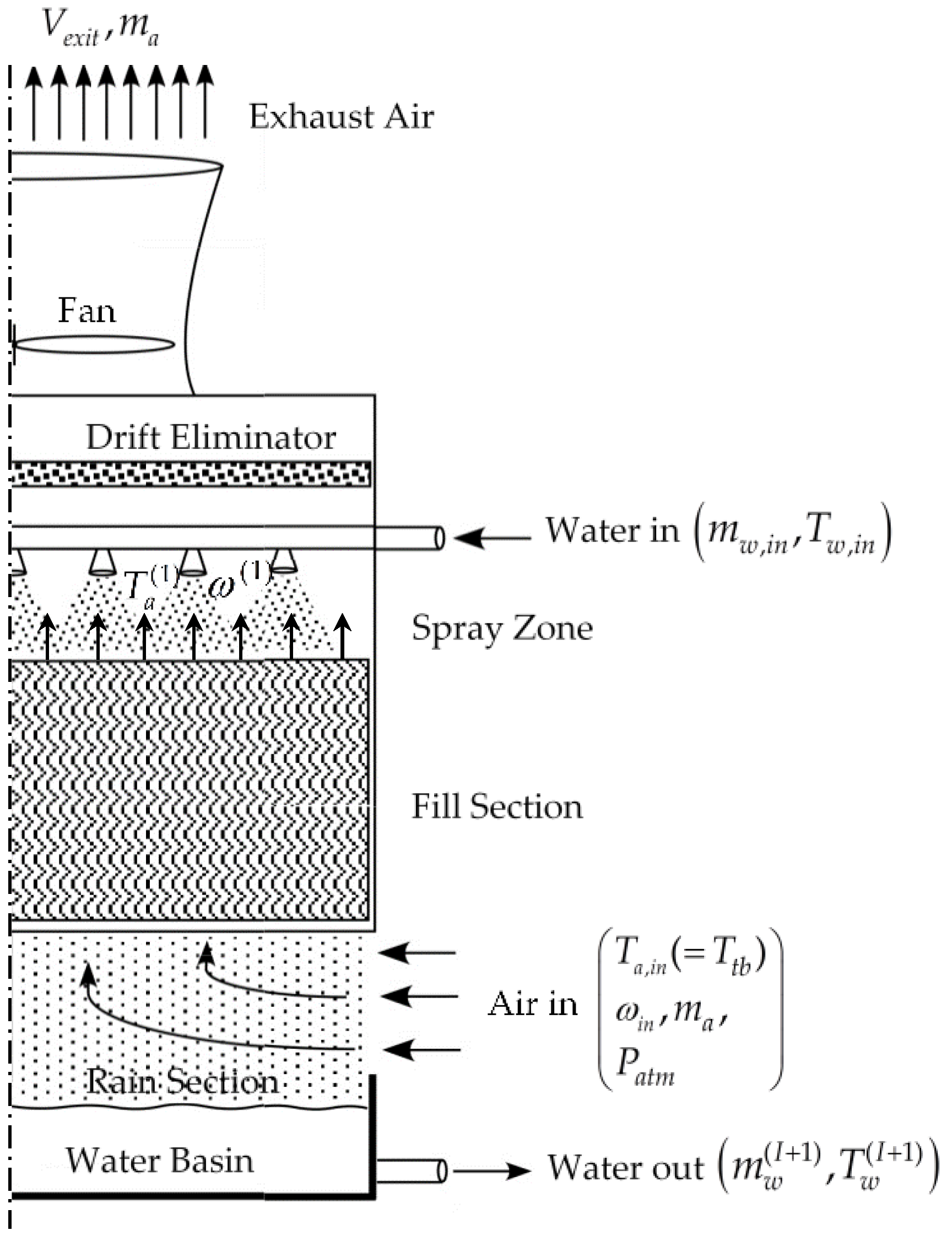
The counter-flow cooling tower considered in this work has been originally developed in [1] and is schematically presented in Figure 1.

As this figure indicates, forced air flow enters the tower through the “rain section” above the water basin, flows upward through the fill section and the drift eliminator, and exits at the tower’s top through an exhaust that encloses a fan. Hot water enters above the fill section and is sprayed onto the top of the fill section to create a uniform, downward falling, film flow through the fill’s numerous meandering vertical passages. Film fills are designed to maximize the water free surface area and the residence time inside of the fill section. Heat and mass transfer occurs at the falling film’s free surface between the water film and the upward air flow. The drift eliminator above the spray zone removes entrained water droplets from the upward flowing air. Below the fill section, the water droplets fall into a collection basin, placed at the bottom of the cooling tower. The heat and mass transfer processes occur overwhelmingly in the fill section. Modeling the heat and mass transfer processes between falling water film and rising air in the cooling tower’s fill section is accomplished by solving the following balance equations: (A) liquid continuity; (B) liquid energy balance; (C) water vapor continuity; (D) air/water vapor energy balance. The assumptions used in deriving these equations are as follows:

• the air and/or water temperatures are uniform throughout each stream at any cross section;
• the cooling tower has uniform cross-sectional area;
• the heat and mass transfer occur solely in the direction normal to flows;
• the heat and mass transfer through tower walls to the environment is negligible;
• the heat transfer from the cooling tower fan and motor assembly to the air is negligible;
• the air and water vapor mix as ideal gasses;
• the flow between flat plates is unsaturated through the fill section.

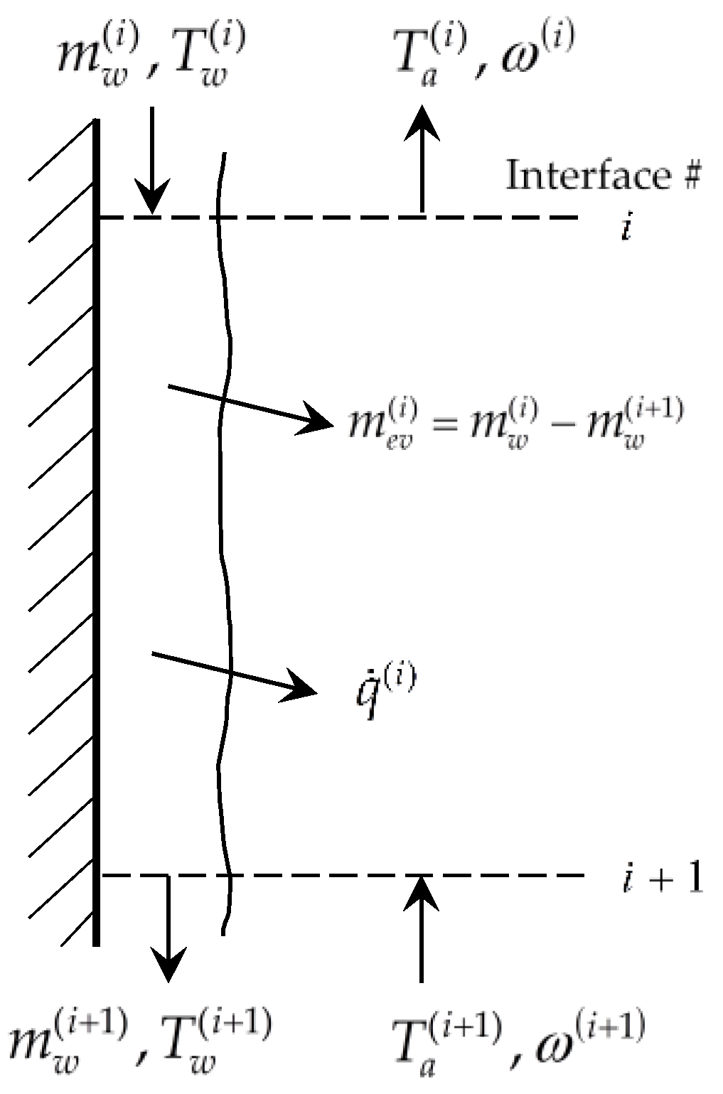
This work considers moderately sized towers for which the heat and mass transfer processes in the rain section is negligible. The fill section is modeled by discretizing it in vertically stacked control volumes as depicted in Figure 2. The heat and mass transfer between the falling water film and the rising air in a typical control volume of the cooling tower’s fill section is presented in Figure 3.

In the mechanical draft mode, the mass flow rate of dry air is specified. With the fan off and hot water flowing through the cooling tower, air will continue to flow through the tower due to buoyancy. Wind pressure at the air inlet to the cooling tower will also enhance air flow through the tower. The air flow rate is determined from the overall mechanical energy equation for the dry air flow. The state functions underlying the cooling tower model (cf., Figure 1, Figure 2 and Figure 3) are as follows:

• the water mass flow rates, denoted as $m_w^{(i)}(i=2,\dots ,50)$, at the exit of each control volume, i, along the height of the fill section of the cooling tower;
• the water temperatures, denoted as $T_w^{(i)}(i=2,\dots ,50)$, at the exit of each control volume, i, along the height of the fill section of the cooling tower;
• the air temperatures, denoted as $T_a^{(i)}(i=1,\dots ,49)$, at the exit of each control volume, i, along the height of the fill section of the cooling tower; and
• the humidity ratios, denoted as .${\omega }^{(i)}(i=1,\dots ,49)$, at the exit of each control volume, i, along the height of the fill section of the cooling tower.

It is convenient to consider the above state functions to be components of the following (column) vectors:

$$m_w\equiv {\left[m_w^{(2)},\dots ,m_w^{(I+1)}\right]}^{†},T_w\equiv {\left[T_w^{(2)},\dots ,T_w^{(I+1)}\right]}^{†},T_a\equiv {\left[T_a^{(1)},\dots ,T_a^{(I)}\right]}^{†},\mathsf{\omega }\equiv {\left[{\mathsf{\omega }}^{(1)},\dots ,{\mathsf{\omega }}^{(I)}\right]}^{†}$$

(1)

In this work, the dagger $(+)$ will be used to denote “transposition”, and all vectors will be considered to be column vectors. The governing conservation equations within the total of I = 49 control volumes represented in Figure 2 are as follows [1]:

• Liquid continuity equations:

  (i) 

  Control Volume i = 1:

  $$N_1^{(1)}\left(m_w,T_w,T_a,\mathsf{\omega };\mathit{\alpha }\right)\triangleq m_w^{(2)}-m_{w,in}+\frac{M(m_a,\mathit{\alpha })}{\overline{R}}\left[\frac{P_{vs}^{(2)}(T_w^{(2)},\mathit{\alpha })}{T_w^{(2)}}-\frac{{\mathsf{\omega }}^{(1)}{P}_{atm}}{T_a^{(1)}(0.622+{\mathsf{\omega }}^{(1)})}\right]=0;$$

  (2)

  (ii) 

  Control Volumes i = 2,..., I−1:

  $$N_1^{\left(i\right)}\left(m_w,T_w,T_a,\mathsf{\omega };\mathit{\alpha }\right)\triangleq m_w^{(i+1)}-m_w^{(i)}+\frac{M(m_a,\mathit{\alpha })}{\overline{R}}\left[\frac{P_{vs}^{(i+1)}(T_w^{(i+1)},\mathit{\alpha })}{T_w^{(i+1)}}-\frac{{\mathsf{\omega }}^{(i)}{P}_{atm}}{T_a^{(i)}(0.622+{\mathsf{\omega }}^{(i)})}\right]=0;$$

  (3)

  (iii) 

  Control Volume i = I:

  $$N_1^{(I)}\left(m_w,T_w,T_a,\mathsf{\omega };\mathit{\alpha }\right)\triangleq m_w^{(I+1)}-m_w^{(I)}+\frac{M(m_a,\mathit{\alpha })}{\overline{R}}\left[\frac{P_{vs}^{(I+1)}(T_w^{(I+1)},\mathit{\alpha })}{T_w^{(I+1)}}-\frac{{\mathsf{\omega }}^{(I)}{P}_{atm}}{T_a^{(I)}(0.622+{\mathsf{\omega }}^{(I)})}\right]=0;$$

  (4)

• Liquid energy balance equations:

  (i) 

  Control Volume i = 1:

  $$\begin{array}{ll}\hfill N_2^{(1)}(m_w,T_w,T_a,\mathsf{\omega };\mathit{\alpha }& )\triangleq m_{w,in}{h}_f(T_{w,in},\mathit{\alpha })-(T_w^{(2)}-T_a^{(1)})H(m_a,\mathit{\alpha })\hfill \\ & -m_w^{(2)}{h}_f^{(2)}(T_w^{(2)},\mathit{\alpha })-(m_{w,in}-m_w^{(2)})h_{g,w}^{(2)}(T_w^{(2)},\mathit{\alpha })=0;\hfill \end{array}$$

  (5)

  (ii) 

  Control Volumes i = 2,…, I−1:

  $$\begin{array}{l}{N}_2^{\left(i\right)}\left(m_w,T_w,T_a,\mathsf{\omega };\mathit{\alpha }\right)\triangleq m_w^{(i)}{h}_f^{(i)}(T_w^{(i)},\mathit{\alpha })-(T_w^{(i+1)}-T_a^{(i)})H(m_a,\mathit{\alpha })\\ -m_w^{(i+1)}{h}_f^{(i+1)}(T_w^{(i+1)},\mathit{\alpha })-(m_w^{(i)}-m_w^{(i+1)})h_{g,w}^{(i+1)}(T_w^{(i+1)},\mathit{\alpha })=0;\end{array}$$

  (6)

  (iii) 

  Control Volume i = I:

  $$\begin{array}{l}{N}_2^{(I)}\left(m_w,T_w,T_a,\mathsf{\omega };\mathit{\alpha }\right)\triangleq m_w^{(I)}{h}_f^{(I)}(T_w^{(I)},\mathit{\alpha })-(T_w^{(I+1)}-T_a^{(I)})H(m_a,\mathit{\alpha })\\ -m_w^{(I+1)}{h}_f^{(I+1)}(T_w^{(I+1)},\mathit{\alpha })-(m_w^{(I)}-m_w^{(I+1)})h_{g,w}^{(I+1)}(T_w^{(I+1)},\mathit{\alpha })=0;\end{array}$$

  (7)

• Water vapor continuity equations:

  (i) 

  Control Volume i = 1:

  $$N_3^{(1)}\left(m_w,T_w,T_a,\mathsf{\omega };\mathit{\alpha }\right)\triangleq {\mathsf{\omega }}^{(2)}-{\mathsf{\omega }}^{(1)}+\frac{m_{w.in}-m_w^{(2)}}{\left|m_a\right|}=0;$$

  (8)

  (ii) 

  Control Volumes i = 2,..., I−1:

  $$N_3^{\left(i\right)}\left(m_w,T_w,T_a,\mathsf{\omega };\mathit{\alpha }\right)\triangleq {\mathsf{\omega }}^{(i+1)}-{\mathsf{\omega }}^{(i)}+\frac{m_w^{(i)}-m_w^{(i+1)}}{\left|m_a\right|}=0;$$

  (9)

  (iii) 

  Control Volume i = I:

  $$N_3^{(I)}\left(m_w,T_w,T_a,\mathsf{\omega };\mathit{\alpha }\right)\triangleq {\mathsf{\omega }}_{in}-{\mathsf{\omega }}^{(I)}+\frac{m_w^{(I)}-m_w^{(I+1)}}{\left|m_a\right|}=0;$$

  (10)

• The air/water vapor energy balance equations:

  (i) 

  Control Volume i = 1:

  $$\begin{array}{l}{N}_4^{(1)}\left(m_w,T_w,T_a,\mathsf{\omega };\mathit{\alpha }\right)\triangleq (T_a^{(2)}-T_a^{(1)})C_p^{(1)}(\frac{T_a^{(1)}+273.15}{2},\mathit{\alpha })-{\mathsf{\omega }}^{(1)}{h}_{g,a}^{(1)}(T_a^{(1)},\mathit{\alpha })\\ +\frac{(T_w^{(2)}-T_a^{(1)})H(m_a,\mathit{\alpha })}{\left|m_a\right|}+\frac{(m_{w,in}-m_w^{(2)})h_{g,w}^{(2)}(T_w^{(2)},\mathit{\alpha })}{\left|m_a\right|}+{\mathsf{\omega }}^{(2)}{h}_{g,a}^{(2)}(T_a^{(2)},\mathit{\alpha })=0;\end{array}$$

  (11)

  (ii) 

  Control Volumes i = 2,..., I−1:

  $$\begin{array}{l}{N}_4^{(i)}\left(m_w,T_w,T_a,\mathsf{\omega };\mathit{\alpha }\right)\triangleq (T_a^{(i+1)}-T_a^{(i)})C_p^{(i)}(\frac{T_a^{(i)}+273.15}{2},\mathit{\alpha })-{\mathsf{\omega }}^{(i)}{h}_{g,a}^{(i)}(T_a^{(i)},\mathit{\alpha })\\ +\frac{(T_w^{(i+1)}-T_a^{(i)})H(m_a,\mathit{\alpha })}{\left|m_a\right|}+\frac{(m_w^{(i)}-m_w^{(i+1)})h_{g,w}^{(i+1)}(T_w^{(i+1)},\mathit{\alpha })}{\left|m_a\right|}+{\mathsf{\omega }}^{(i+1)}{h}_{g,a}^{(i+1)}(T_a^{(i+1)},\mathit{\alpha })=0;\end{array}$$

  (12)

  (iii) 

  Control Volume i = I:

  $$\begin{array}{l}{N}_4^{(I)}\left(m_w,T_w,T_a,\mathsf{\omega };\mathit{\alpha }\right)\triangleq (T_{a,in}-T_a^{(I)})C_p{}^{(I)}(\frac{T_a^{(I)}+273.15}{2},\mathit{\alpha })-{\mathsf{\omega }}^{(I)}{h}_{g,a}^{(I)}(T_a^{(I)},\mathit{\alpha })\\ +\frac{(T_w^{(I+1)}-T_a^{(I)})H(m_a,\mathit{\alpha })}{\left|m_a\right|}+\frac{(m_w^{(I)}-m_w^{(I+1)})h_{g,w}^{(I+1)}(T_w^{(I+1)},\mathit{\alpha })}{\left|m_a\right|}+{\mathsf{\omega }}_{in}{h}_{g,a}(T_{a,in},\mathit{\alpha })=0.\end{array}$$

  (13)

The components of the vector $\mathit{\alpha }$, which appears in Equations (2)–(13), comprise the model parameters which are generically denoted as ${\alpha }_i$, i.e.:

$$\mathit{\alpha }\triangleq \left({\alpha }_1,\dots ,{\alpha }_{N_{\alpha }}\right),$$

(14)

where $N_{\alpha }$ denotes the total number of model parameters. These model parameters are experimentally derived quantities, and their complete distributions parameters are not known; however, we have determined the first four moments (means, variance/covariance, skewness, and kurtosis) of each of these parameter distributions, as detailed in Appendix B.

In the original work [1], the above equations were solved using a two stage-iterative method comprising an “inner-iteration” using Newton’s method within each control volume, followed by an outer iteration aimed at achieving overall convergence. This procedure, though, did not converge at all of the points of interest. Therefore, after testing several alternatives provided in [8] and [9], we have replaced the original solution method in [1] by Newton’s method together with the GMRES linear iterative solver for sparse matrices [10] provided in the NSPCG package [9], which turned out to be the most efficient among those we have tested. This GMRES method [10] approximates the exact solution-vector of a linear system by using the Arnoldi iteration to find the approximate solution-vector by minimizing the norm of the residual vector over a Krylov subspace. The specific computational steps are as follows:

(a)

Write Equations (1)–(13) in vector form as:

$$N\left(u\right)=0,$$

(15)

where the following definitions were used:

$$N\triangleq {\left(N_1^{(1)},..,N_1^{(I)},\dots ,N_4^{(1)},\dots ,N_4^{(I)}\right)}^{†},u\triangleq {\left(m_w,T_w,T_a,\mathsf{\omega }\right)}^{†}$$

(16)

(b)

Set the initial guess, $u_0$, to be the inlet boundary conditions;

(c)

Steps d through g, below, constitute the outer iteration loop; for $n=0,1,2,\dots$, iterate over the following steps until convergence:

(d)

Inner iteration loop: for $m=1,2,\dots ,$ use the iterative GMRES linear solver with the Modified Incomplete Cholesky (MIC) preconditioner, with restarts, to solve, until convergence, the following system to compute the vector $\delta u$:

$$J\left(u_n\right)\delta u=-N\left(u_n\right),$$

(17)

where $n$ is the current outer loop iteration number, and the Jacobian matrix of derivatives of Equations (2)–(13) with respect to the state functions is the block-matrix:

$$J\left(u_n\right)\triangleq \left(\begin{array}{cccc}{A}_1& B_1& C_1& D_1\\ A_2& B_2& C_2& D_2\\ A_3& B_3& C_3& D_3\\ A_4& B_4& C_4& D_4\end{array}\right),$$

(18)

with matrix-components defined in Appendix C. As shown in this Appendix, the Jacobian represented by Equation (18) is a non-symmetric sparse matrix of order 196 by 196, with 14 nonzero diagonals. The non-symmetric diagonal storage format is used to store the respective 14 nonzero diagonals, so that the “condensed” Jacobian matrix has dimensions 196 by 14. Since the Jacobian is highly non-symmetric, the cost of the iterations of the GMRES solver grows as O(m²), where m is the iteration number within the GMRES solver. To reduce this computational cost, the GMRES solver is configured to run with the restart feature. The optimized value for the restart frequency is 10 for this specific application. The MIC preconditioner can speed up the convergence of the GMRES solver using the parameters OMEGA and LVFILL [9] in the modified incomplete factorization methods for the MIC preconditioner; for this application the following values were found to be optimal: OMEGA = 0.000000001 and LVFILL = 1. The Jacobian is not updated inside the sparse GMRES solver. The default convergence of GMRES is tested with the following criterion [9]:

$${\left[\frac{\langle {\tilde{z}}^{(m)},{\tilde{z}}^{(m)}\rangle }{\langle \delta u^{(m)},\delta u^{(m)}\rangle }\right]}^{\frac{1}{2}}<\zeta$$

(19)

where ${\tilde{z}}^{(m)}$ denotes the pseudo-residual at m^th-iteration of the GMRES solver, $\delta u^{(m)}$ is the solution of Equation (17) at m^th-iteration, and $\zeta$ denotes the stopping test value for the GMRES solver.

(e)

Set

$$u_{n+1}=u_n+\delta u,$$

(20)

where $n$ is the current outer loop iteration number, and update the Jacobian.

(f)

Test for convergence of the outer loop until the error in the solution is less than a specified maximum value. For solving Equations (2)–(13), the following error criterion has been used:

$$error=\max \left(\frac{\left|\delta m_w^{(i)}\right|}{m_w^{(i)}},\frac{\left|\delta T_w^{(i)}\right|}{T_w^{(i)}},\frac{\left|\delta T_a^{(i)}\right|}{T_a^{(i)}},\frac{\left|\delta {\omega }^{(i)}\right|}{{\omega }^{(i)}}\right)<{10}^{-6}$$

(g)

Set $n=n+1$ and go to step d.

The above solution strategy for solving Equations (2)–(13) converged successfully for all the 8079 benchmark data sets. As described previously, each of these data sets contained measurements of the following quantities: (i) outlet air temperature measured with the sensor called “Tidbit”; (ii) outlet air temperature measured with the sensor called “Hobo”; (iii) outlet water temperature; (iv) outlet air relative humidity. For each of these benchmark data sets, the outer loop iterations described above (i.e., steps c through g) converge in 4 iterations; for each outer loop iteration, the GMRES solver used for solving Equation (17) converges in 12 iterations. The “zero-to-zero” verification of the solution’s accuracy using Equations (2) through (13) gives an error of the order of ${10}^{-7}$.

In view of the above-mentioned measurements, the responses of interest for this work are as follows:

(a)

the vector $m_w\triangleq {\left[m_w^{(2)},\dots ,m_w^{(I+1)}\right]}^{†}$ of water mass flow rates at the exit of each control volume i, $(i=1,\dots ,49)$;

(b)

the vector $T_w\triangleq {\left[T_w^{(2)},\dots ,T_w^{(I+1)}\right]}^{†}$ of water temperatures at the exit of each control volume i, $(i=1,\dots ,49)$;

(c)

the vector $T_a\triangleq {\left[T_a^{(1)},\dots ,T_a^{(I)}\right]}^{†}$ of air temperatures at the exit of each control volume i, $(i=1,\dots ,49)$;

(d)

the vector $RH\triangleq {\left[R{H}^{(1)},\dots ,R{H}^{(I)}\right]}^{†}$, having components of the air relative humidity at the exit of each control volume i, $(i=1,\dots ,49)$.

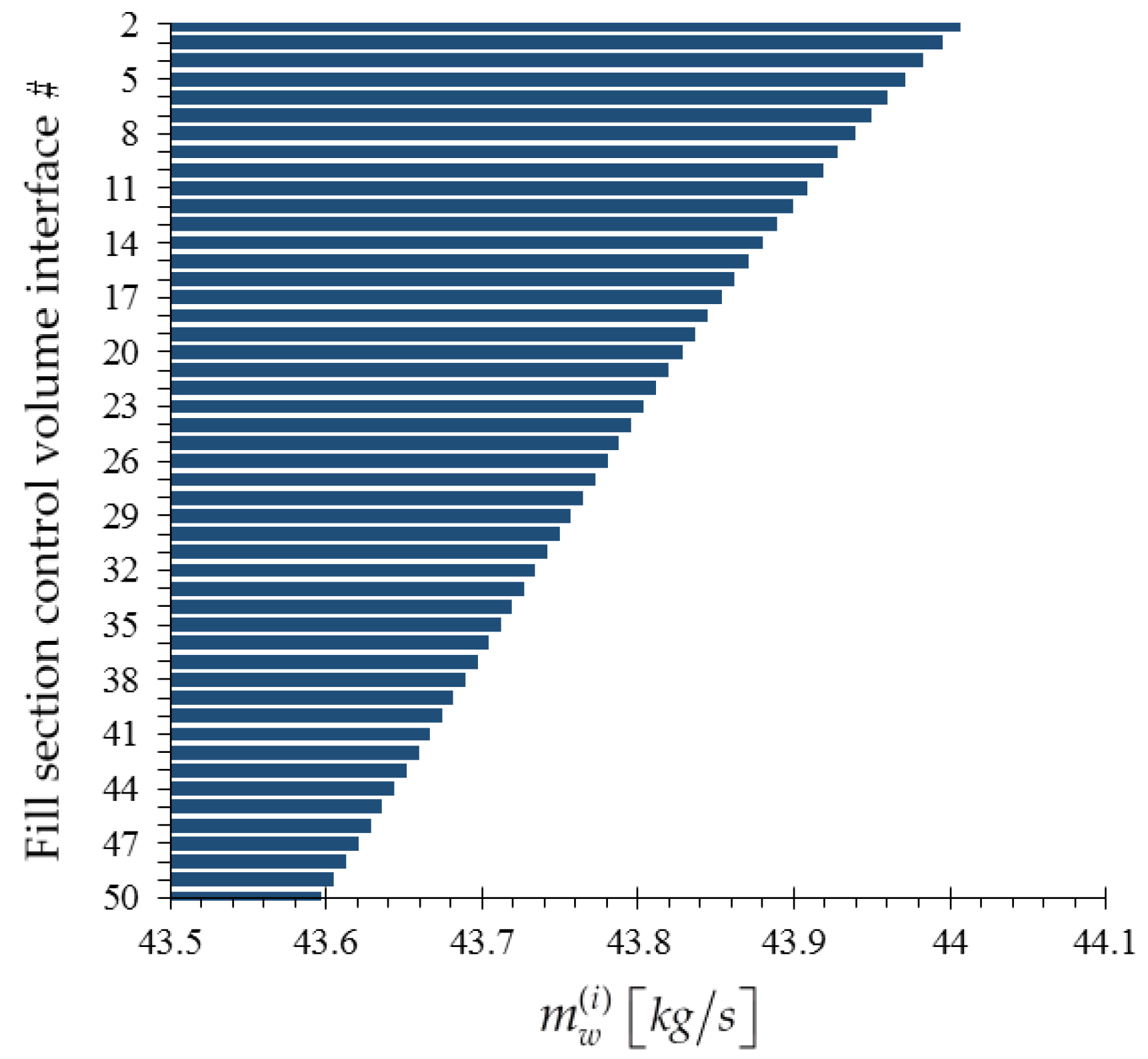
While the water mass flow rates $m_w^{(i)}$, the water temperatures $T_w^{(i)}$, and the air temperatures $T_a^{(i)}$ are obtained directly as the solutions of Equations (2)–(13), the air relative humidity, $R{H}^{(i)}$, is computed for each control volume using the expression:

$$R{H}^{(i)}=\frac{P_v\left({\mathsf{\omega }}^{(i)},\mathit{\alpha }\right)}{P_{vs}\left(T_a^{(i)},\mathit{\alpha }\right)}\times 100=\frac{\left(\frac{{\mathsf{\omega }}^{(i)}{P}_{atm}}{{\mathsf{\omega }}^{(i)}+0.622}\right)}{\left(e^{a_0+\frac{a_1}{T_a^{(i)}}}\right)}\times 100.$$

(21)

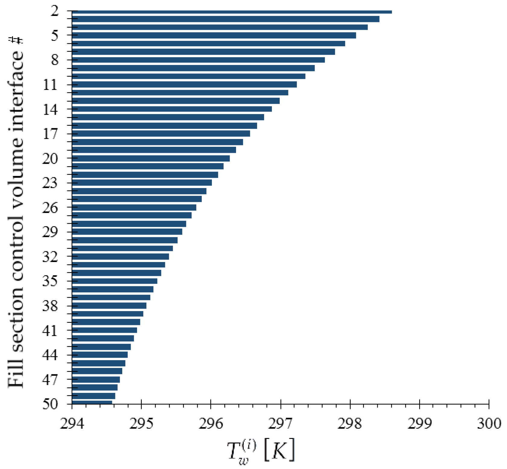
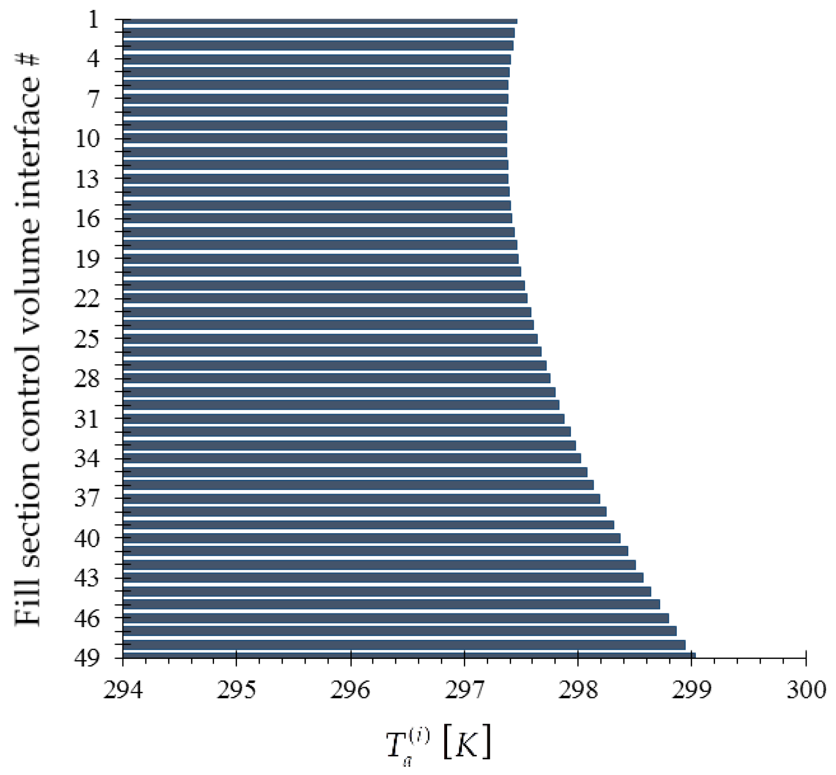
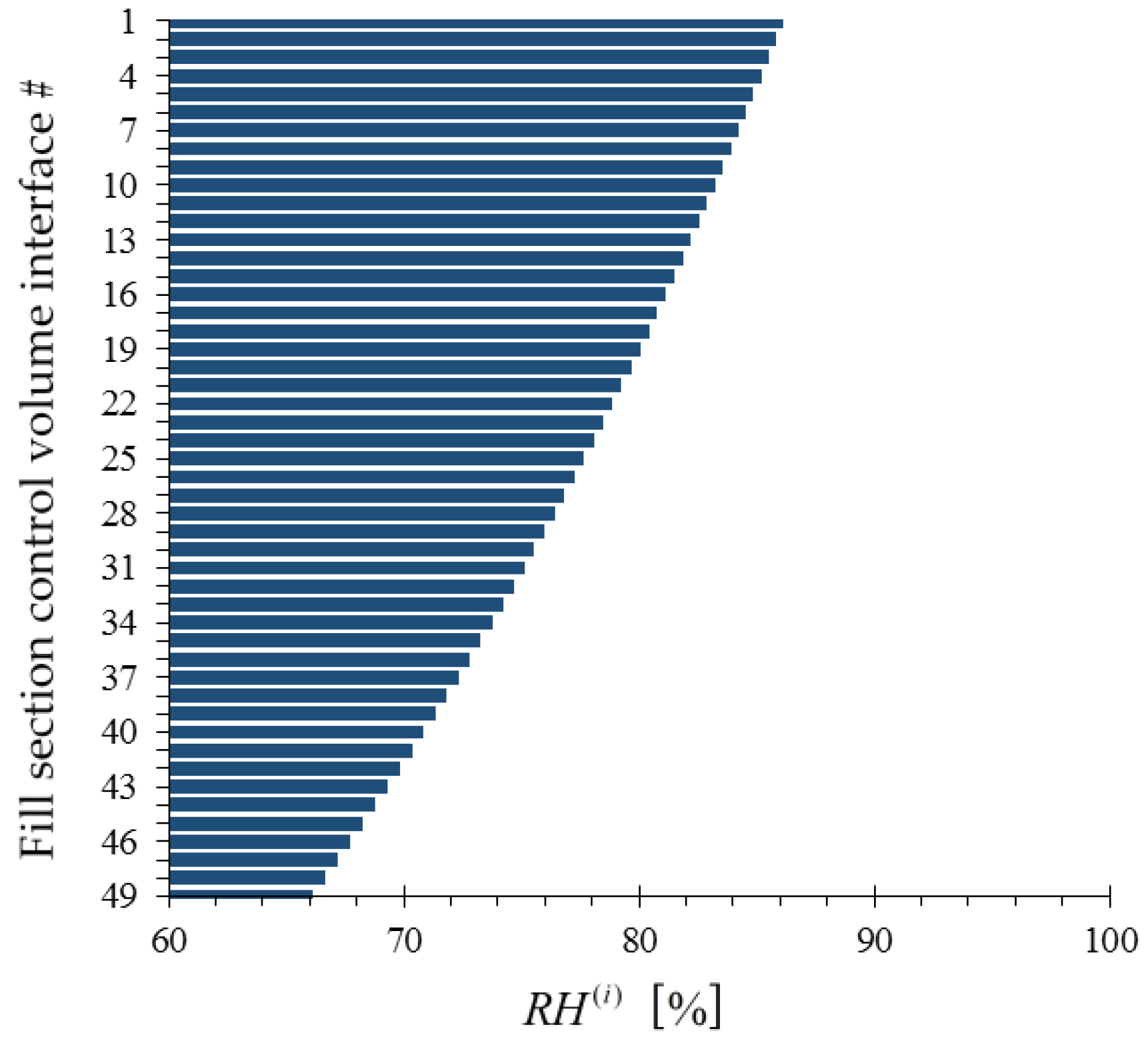
The bar plots, showing the respective values of the water mass flow rates $m_w^{(i)}$, the water temperatures $T_w^{(i)}$, the air temperatures $T_a^{(i)}$, and the air relative humidity, $R{H}^{(i)}$, at the exit of each control volume, are presented in Figure 4, Figure 5, Figure 6 and Figure 7, below.

2.2. Development of the Cooling Tower Adjoint Sensitivity Model, with Solution Verification

All of the responses of interest in this work, e.g., the experimentally measured and/or computed responses discussed in the previous Sections, can be generally represented in the functional form $R\left(m_w,T_w,T_a,\mathsf{\omega };\mathit{\alpha }\right)$, where $R$ is a known functional of the model’s state functions and parameters. As generally shown in [2], the sensitivity of such as this response to arbitrary variations in the model’s parameters $\delta \mathit{\alpha }\equiv \left(\delta {\alpha }_1,\dots ,\delta {\alpha }_{N_{\alpha }}\right)$ and state functions $\delta m_w,\delta T_w,\delta T_a,\delta \mathsf{\omega }$ is provided by the response’s Gateaux (G-) differential $DR\left(m_w^0,T_w^0,T_a^0,{\mathsf{\omega }}^0;{\mathit{\alpha }}^0;\delta m_w,\delta T_w,\delta T_a,\delta \mathsf{\omega };\delta \mathit{\alpha }\right)$, which is defined as follows:

$$\begin{array}{l}DR\left(m_w^0,T_w^0,T_a^0,{\mathsf{\omega }}^0;{\mathit{\alpha }}^0;\delta m_w,\delta T_w,\delta T_a,\delta \mathsf{\omega };\delta \mathit{\alpha }\right)\triangleq \\ \frac{d}{d\epsilon }{\left[R\left(m_w^0+\epsilon \delta m_w,T_w^0+\epsilon \delta T_w,T_a^0+\epsilon \delta T_a,{\mathsf{\omega }}^0+\epsilon \delta \mathsf{\omega };{\mathit{\alpha }}^0+\epsilon \delta \mathit{\alpha }\right)\right]}_{\epsilon =0}\\ =D{R}_{direct}+D{R}_{indirect},\end{array}$$

(22)

where the so-called “direct effect” term, $D{R}_{direct}$, and the so-called “indirect effect” term, $D{R}_{indirect}$, are defined, respectively, as follows:

$$D{R}_{direct}\equiv {\displaystyle \sum _{i=1}^{N_{\alpha }}\left(\frac{\partial R}{\partial {\alpha }_i}\delta {\alpha }_i\right)},$$

(23)

$$\begin{array}{ll}\hfill D{R}_{indirect}& \triangleq {\displaystyle \sum _{i=1}^I\left(\frac{\partial R}{\partial m_w^{\left(i+1\right)}}\delta m_w^{\left(i+1\right)}+\frac{\partial R}{\partial T_w^{\left(i+1\right)}}\delta T_w^{\left(i+1\right)}+\frac{\partial R}{\partial T_a^{\left(i\right)}}\delta T_a^{\left(i\right)}+\frac{\partial R}{\partial {\omega }^{\left(i\right)}}\delta {\omega }^{\left(i\right)}\right)}\hfill \\ & =R_1\cdot \delta m_w+R_2\cdot \delta T_w+R_3\cdot \delta T_a+R_4\cdot \delta \mathsf{\omega },\hfill \end{array}$$

(24)

where the components of the vectors $R_{\ell }\equiv \left(r_{\ell }^{\left(1\right)},\dots ,r_{\ell }^{\left(I\right)}\right),\ell =1,2,3,4$ are defined as follows:

$$r_1^{\left(i\right)}\equiv \frac{\partial R}{\partial m_w^{\left(i+1\right)}};r_2^{\left(i\right)}\equiv \frac{\partial R}{\partial T_w^{\left(i+1\right)}};r_3^{\left(i\right)}\equiv \frac{\partial R}{\partial T_a^{\left(i\right)}};r_4^{\left(i\right)}\equiv \frac{\partial R}{\partial {\omega }^{\left(i\right)}};i=1,\dots ,I.$$

(25)

Since the model parameters are related to the model’s state functions through Equations (2)–(13), it follows that variations in the model parameter will induce variations in the state variables. More precisely, it has been shown in [2,3,4] that to first-order in the parameter variations, the respective variations in the state variables can be computed by solving the G-differentiated model equations, namely:

$$\frac{d}{d\epsilon }{\left[N\left(u^0+\epsilon \delta u;{\mathit{\alpha }}^0+\epsilon \delta \mathit{\alpha }\right)\right]}_{\epsilon =0}=0,$$

Performing the above differentiation on Equations (2) through (13) yields the following forward sensitivity system:

$$\left(\begin{array}{cccc}{A}_1& B_1& C_1& D_1\\ A_2& B_2& C_2& D_2\\ A_3& B_3& C_3& D_3\\ A_4& B_4& C_4& D_4\end{array}\right)\left(\begin{array}{c}\delta m_w\\ \delta T_w\\ \delta T_a\\ \delta \mathsf{\omega }\end{array}\right)=\left(\begin{array}{c}{Q}_1\\ Q_2\\ Q_3\\ Q_4\end{array}\right),$$

(26)

where the components of the vectors $Q_{\ell }\equiv \left(q_{\ell }^{\left(1\right)},\dots ,q_{\ell }^{\left(I\right)}\right),\ell =1,2,3,4$ are defined as follows:

$$q_{\ell }^{\left(i\right)}\equiv {\displaystyle \sum _{j=1}^{N_{\alpha }}\left(\frac{\partial N_{\ell }^{\left(i\right)}}{\partial {\alpha }_j}\delta {\alpha }_j\right)};i=1,\dots ,I;\ell =1,2,3,4.$$

(27)

The system represented by Equation (26) is called the forward sensitivity system, which can be solved, in principle, to compute the variations in the state functions for every variation in the model parameters. In turn, the solution of Equation (26) can be used in Equation (24) to compute the “indirect effect” term, $D{R}_{indirect}$. However, since there are many parameter variations to consider, solving Equation (26) repeatedly to compute $D{R}_{indirect}$ becomes computationally impracticable. The need for solving Equation (26) repeatedly to compute $D{R}_{indirect}$ can be circumvented by applying the Adjoint Sensitivity Analysis Procedure (ASAM) formulated in [2,3,4]. The ASAM proceeds by forming the inner-product of Equation (26) with a yet unspecified vector of the form ${\left[{\mathsf{\mu }}_w,{\mathsf{\tau }}_w,{\mathsf{\tau }}_a,o\right]}^{†}$, having the same structure as the vector $u\triangleq {\left(m_w,T_w,T_a,\mathsf{\omega }\right)}^{†}$, transposing the resulting scalar equation and using Equation (24). Furthermore, by requiring that the vector ${\left[{\mathsf{\mu }}_w,{\mathsf{\tau }}_w,{\mathsf{\tau }}_a,o\right]}^{†}$ satisfy the following adjoint sensitivity system:

$$\left(\begin{array}{cccc}{A}_1^{†}& A_2^{†}& A_3^{†}& A_4^{†}\\ B_1^{†}& B_2^{†}& B_3^{†}& B_4^{†}\\ C_1^{†}& C_2^{†}& C_3^{†}& C_4^{†}\\ D_1^{†}& D_2^{†}& D_3^{†}& D_4^{†}\end{array}\right)\left(\begin{array}{c}{\mathsf{\mu }}_w\\ {\mathsf{\tau }}_w\\ {\mathsf{\tau }}_a\\ o\end{array}\right)=\left(\begin{array}{c}{R}_1\\ R_2\\ R_3\\ R_4\end{array}\right),$$

(28)

it ultimately results that the “indirect effect” term can be expressed in the form

$$D{R}_{indirect}\equiv {\mathsf{\mu }}_w\cdot Q_1+{\mathsf{\tau }}_w\cdot Q_2+{\mathsf{\tau }}_a\cdot Q_3+o\cdot Q_4$$

(29)

The system represented by Equation (28) is called the adjoint sensitivity system, which –notably– is independent of parameter variations. Therefore, the adjoint sensitivity system needs to be solved only once, to compute the adjoint functions ${\left[{\mathsf{\mu }}_w,{\mathsf{\tau }}_w,{\mathsf{\tau }}_a,o\right]}^{†}$. In turn, the adjoint functions are used to compute $D{R}_{indirect}$, efficiently and exactly, using Equation (29). As an illustrative example of computing response sensitivities using the adjoint sensitivity system, consider that the model response of interest is the air relative humidity, $R{H}^{(i)}$, in a generic control volume i, as given by Equation (21). For this model response, the “direct effect” term, denoted as $D{\left[R{H}^{(i)}\right]}_{direct}$, is readily obtained in the form:

$$D{\left[R{H}^{(i)}\right]}_{direct}=\frac{\partial \left(R{H}^{(i)}\right)}{\partial P_{atm}}\left(\delta P_{atm}\right)+\frac{\partial \left(R{H}^{(i)}\right)}{\partial a_0}\left(\delta a_0\right)+\frac{\partial \left(R{H}^{(i)}\right)}{\partial a_1}\left(\delta a_1\right),i=1,\dots ,I;$$

(30)

where:

$$\frac{\partial \left(R{H}^{(i)}\right)}{\partial P_{atm}}=\frac{\partial }{\partial P_{atm}}\left[\frac{P_v\left({\mathsf{\omega }}^{(i)},\mathit{\alpha }\right)}{P_{vs}\left(T_a^{(i)},\mathit{\alpha }\right)}\times 100\right]=\frac{0.622}{\left(0.622+{\mathsf{\omega }}^{(i)}\right)e^{a_0+\frac{a_1}{T_a^{(i)}}}}\times 100;i=1,\dots ,I;$$

(31)

$$\frac{\partial \left(R{H}^{(i)}\right)}{\partial a_0}=\frac{\partial }{\partial a_0}\left[\frac{P_v\left({\mathsf{\omega }}^{(i)},\mathit{\alpha }\right)}{P_{vs}\left(T_a^{(i)},\mathit{\alpha }\right)}\times 100\right]=-\frac{0.622P_{atm}}{\left(0.622+{\mathsf{\omega }}^{(i)}\right)e^{a_0+\frac{a_1}{T_a^{(i)}}}}\times 100;i=1,\dots ,I;$$

(32)

$$\frac{\partial \left(R{H}^{(i)}\right)}{\partial a_1}=\frac{\partial }{\partial a_1}\left[\frac{P_v\left({\mathsf{\omega }}^{(i)},\mathit{\alpha }\right)}{P_{vs}\left(T_a^{(i)},\mathit{\alpha }\right)}\times 100\right]=-\frac{0.622P_{atm}}{\left(0.622+{\mathsf{\omega }}^{(i)}\right)e^{a_0+\frac{a_1}{T_a^{(i)}}}}\frac{-1}{T_a^{(i)}}\times 100;i=1,\dots ,I.$$

(33)

On the other hand, the “indirect effect” term, denoted as $D{\left[R{H}^{(i)}\right]}_{indirect}$, is readily obtained in the form:

$$D{\left[R{H}^{(i)}\right]}_{indirect}=\frac{\partial \left(R{H}^{(i)}\right)}{\partial {\omega }^{\left(i\right)}}\left(\delta {\omega }^{\left(i\right)}\right)+\frac{\partial \left(R{H}^{(i)}\right)}{\partial T_a^{(i)}}\left(\delta T_a^{(i)}\right);i=1,\dots ,I;$$

(34)

where:

$$\begin{array}{ll}\frac{\partial \left(R{H}^{(i)}\right)}{\partial {\omega }^{\left(i\right)}}& =\frac{\partial }{\partial {\omega }^{\left(i\right)}}\left[\frac{P_v\left({\mathsf{\omega }}^{(i)},\mathit{\alpha }\right)}{P_{vs}\left(T_a^{(i)},\mathit{\alpha }\right)}\times 100\right]=\frac{100}{P_{vs}\left(T_a^{(i)},\mathsf{\alpha }\right)}\frac{\partial P_v\left({\mathsf{\omega }}^{(i)},\mathit{\alpha }\right)}{\partial {\omega }^{\left(i\right)}}\\ & =\frac{0.622P_{atm}}{{\left(0.622+{\omega }^{\left(i\right)}\right)}^2{e}^{a_0+\frac{a_1}{T_a^{(i)}}}}\times 100;i=1,\dots ,I;\end{array}$$

(35)

$$\begin{array}{ll}\frac{\partial \left(R{H}^{(i)}\right)}{\partial T_a^{(i)}}& =\frac{\partial }{\partial T_a^{(i)}}\left[\frac{P_v\left({\mathsf{\omega }}^{(i)},\mathit{\alpha }\right)}{P_{vs}\left(T_a^{(i)},\mathit{\alpha }\right)}\times 100\right]=100\times P_v\left({\mathsf{\omega }}^{(i)},\mathit{\alpha }\right)\frac{\partial }{\partial T_a^{(i)}}\left[\frac{1}{P_{vs}\left(T_a^{(i)},\mathit{\alpha }\right)}\right]\\ & =\frac{0.622P_{atm}}{\left(0.622+{\mathsf{\omega }}^{(i)}\right)e^{a_0+\frac{a_1}{T_a^{(i)}}}}\frac{a_1}{{\left[T_a^{(i)}\right]}^2}\times 100;i=1,\dots ,I.\end{array}$$

(36)

The units of the adjoint functions can be determined from Equation (29) through dimensional analysis. Specifically, the units for the adjoint functions satisfy the following relation:

$$\left[{\mu }_w^{\left(i\right)}\right]=\frac{\left[R\right]}{\left[N_1\right]};\left[{\tau }_w^{\left(i\right)}\right]=\frac{\left[R\right]}{\left[N_2\right]};\left[{\tau }_a^{\left(i\right)}\right]=\frac{\left[R\right]}{\left[N_3\right]};\left[o^{\left(i\right)}\right]=\frac{\left[R\right]}{\left[N_4\right]},$$

(37)

where ”[R]” denotes the unit of the response R, while the units for the respective equations are as follows:

$$\left[N_1\right]=\frac{kg}{s};\left[N_2\right]=\frac{J}{s};\left[N_3\right]=[-];\left[N_4\right]=\frac{J}{kg}.$$

(38)

Table 1. Units of the adjoint functions for different responses.

Responses	$\mathbf{\left[}{\mathit{\mu }}_{\mathit{w}}^{\mathbf{\left(}\mathit{i}\mathbf{\right)}}\mathbf{\right]}$	$\mathbf{\left[}{\mathit{\tau }}_{\mathit{w}}^{\mathbf{\left(}\mathit{i}\mathbf{\right)}}\mathbf{\right]}$	$\mathbf{\left[}{\mathit{\tau }}_{\mathit{a}}^{\mathbf{\left(}\mathit{i}\mathbf{\right)}}\mathbf{\right]}$	$\mathbf{\left[}{\mathit{o}}^{\mathbf{\left(}\mathit{i}\mathbf{\right)}}\mathbf{\right]}$
$R\triangleq T_a^{(1)}$	$K/\left(kg/s\right)$	$K/(J/s)$	$K$	$K/\left(J/kg\right)$
$R\triangleq T_w^{(50)}$	$K/\left(kg/s\right)$	$K/(J/s)$	$K$	$K/\left(J/kg\right)$
$R\triangleq R{H}^{(1)}$	${\left(kg/s\right)}^{-1}$	${\left(J/s\right)}^{-1}$	$-$	${\left(J/kg\right)}^{-1}$
$R\triangleq m_w^{(50)}$	$-$	${\left(J/kg\right)}^{-1}$	$kg/s$	$\left(kg/s\right)/\left(J/kg\right)$

below lists the units of the adjoint functions for four responses: $R\triangleq T_a^{(1)}$, $R\triangleq T_w^{(50)}$, $R\triangleq R{H}^{(1)}$ and $R\triangleq m_w^{(50)}$, respectively, in which, $T_a^{(1)}$ denotes exit air temperature; $T_w^{(50)}$ denotes exit water temperature; $R{H}^{(1)}$ denotes exit air relative humidity; and $m_w^{(50)}$ denotes exit water mass flow rate.

Note that the adjoint sensitivity system represented by Equation (28) is linear in the adjoint state functions, so it can be solved by using numerical methods appropriate for large-scale sparse linear systems. In particular, we solved it by using NSPCG, a “Package for Solving Large Sparse Linear Systems by Various Iterative Methods” [9]; 12 to 18 iterations sufficed for solving the adjoint system within convergence criterion of $\zeta ={10}^{-12}$. 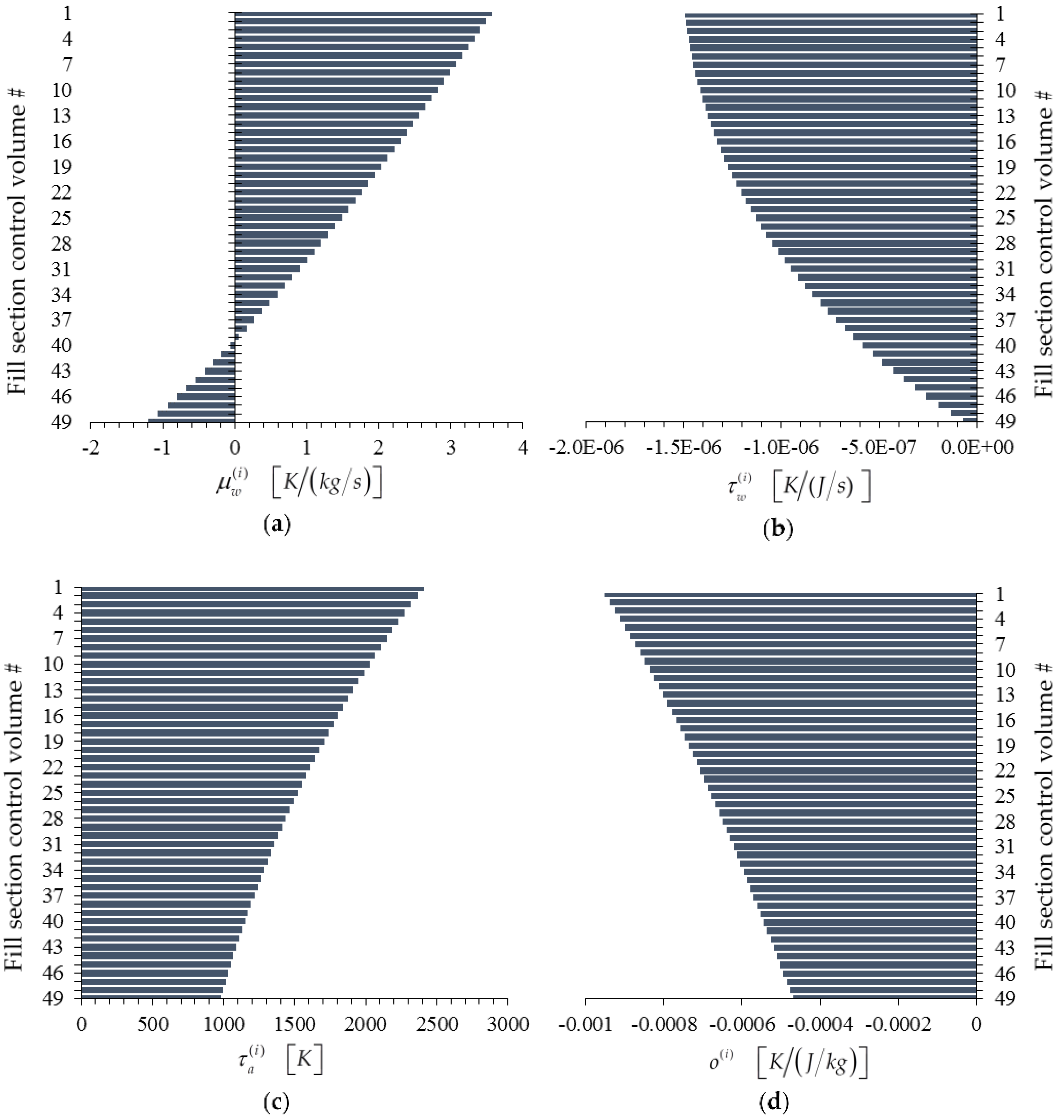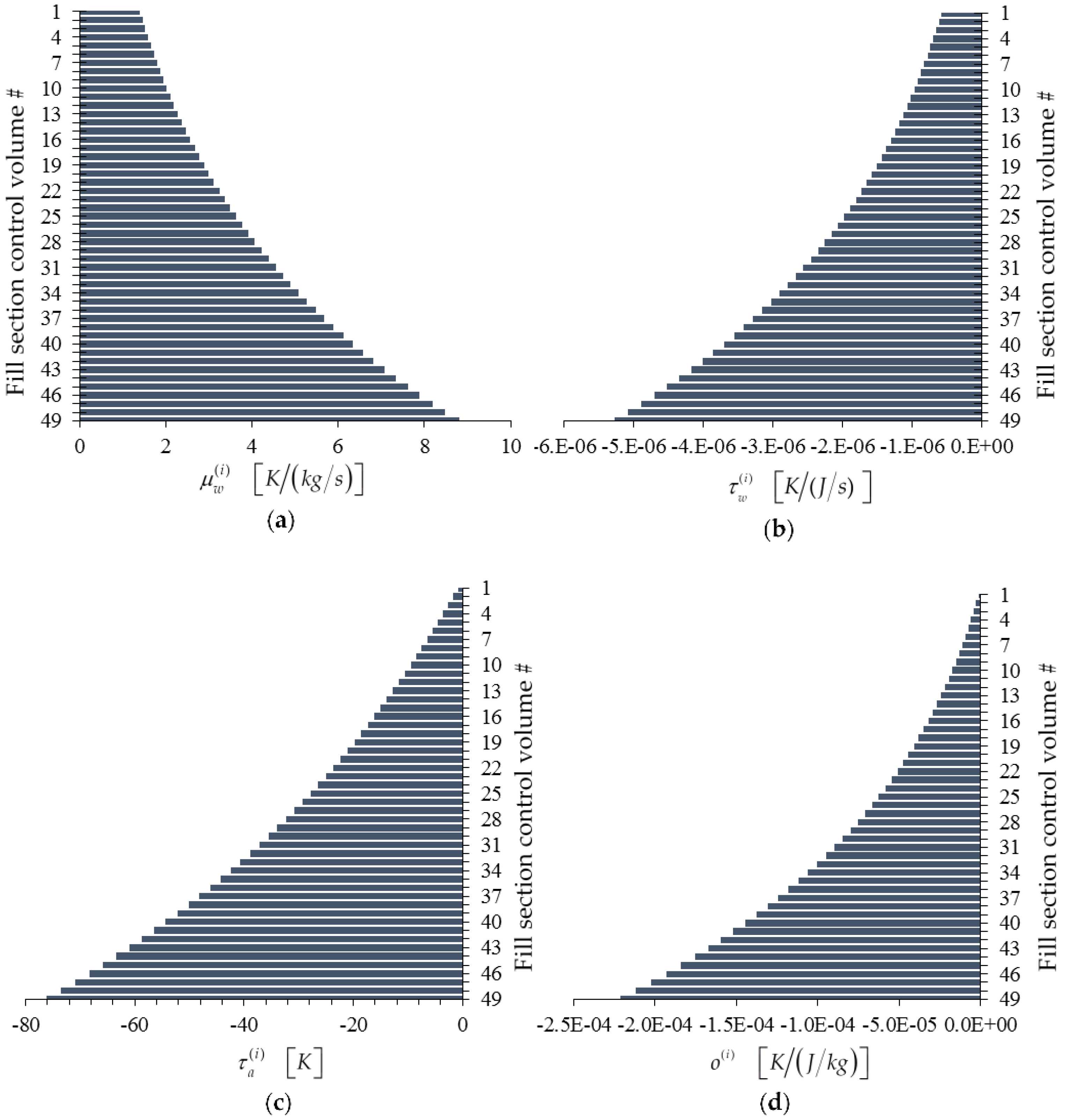The bar plots of the adjoint functions corresponding to the four measured responses of interest, namely: (i) the exit air temperature $R\triangleq T_a^{(1)}$; (ii) the outlet (exit) water temperature $R\triangleq T_w^{(50)}$; (iii) the exit air humidity ratio $R\triangleq R{H}^{(1)}$; and (iv) the outlet (exit) water mass flow rate $R\triangleq m_w^{(50)}$, are presented in Figure 8, Figure 9, Figure 10 and Figure 11.

The numerical accuracy of the computed adjoint functions can be independently verified by first noting that Equations (22), (23) and (29) imply that:

$$DR\left(m_w^0,T_w^0,T_a^0,{\mathsf{\omega }}^0;{\mathit{\alpha }}^0;\delta m_w,\delta T_w,\delta T_a,\delta \mathsf{\omega };\delta \mathit{\alpha }\right)={\displaystyle \sum _{j=1}^{N_{\alpha }}{S}_j}\delta {\alpha }_j,$$

(39)

where $N_{\alpha }$ denotes the total number of model parameters, and $S_j$ denotes the “absolute sensitivity” of the response $R$ with respect to the parameter ${\alpha }_j$, and is defined as:

$$S_j\triangleq \frac{\partial R}{\partial {\alpha }_j}-{\displaystyle \sum _{i=1}^I\left({\mu }_w^{\left(i\right)}\frac{\partial N_1^{\left(i\right)}}{\partial {\alpha }_j}+{\tau }_w^{\left(i\right)}\frac{\partial N_2^{\left(i\right)}}{\partial {\alpha }_j}+{\tau }_a^{\left(i\right)}\frac{\partial N_3^{\left(i\right)}}{\partial {\alpha }_j}+o^{\left(i\right)}\frac{\partial N_4^{\left(i\right)}}{\partial {\alpha }_j}\right)}.$$

(40)

All of the derivatives with respect to the model parameter ${\alpha }_j$ on the right side of Equation (40) are known quantities. On the other hand, the absolute response sensitivity $S_j$ can be computed independently, as follows:

• consider a small perturbation $\delta {\alpha }_j$ in the model parameter ${\alpha }_j$;
• re-compute the perturbed response $R\left({\alpha }_j^0+\delta {\alpha }_j\right)$, where ${\alpha }_j^0$ denotes the unperturbed parameter value;
• use the finite difference formula:

  $$S_j^{FD}\cong \frac{R\left({\alpha }_j^0+\delta {\alpha }_j\right)-R\left({\alpha }_j^0\right)}{\delta {\alpha }_j}+O{\left(\delta {\alpha }_j\right)}^2$$

  (41)
• use the approximate equality between Equations (41) and (40) to obtain independently the respective values of the adjoint function(s) being verified.

The verification procedure described in steps (1)–(4) above, will be illustrated in the remainder of this section, for verifying the adjoint functions depicted in Figure 8, Figure 9, Figure 10 and Figure 11.

2.2.1. Verification of the Adjoint Functions for the Outlet Air Temperature Response $T_a^{(1)}$

When $R=T_a^{(1)}$, the quantities $r_{\ell }^{\left(i\right)}$ defined in Equation (25) all vanish except for a single component, namely: $r_3^{\left(1\right)}\triangleq \partial R/\partial T_a^{\left(1\right)}=1.$ Thus, the adjoint functions corresponding to the outlet air temperature response $T_a^{(1)}$ are computed by solving the adjoint sensitivity system given in Equation (28) using $r_3^{\left(1\right)}\triangleq \partial R/\partial T_a^{\left(1\right)}=1$ as the only non-zero source term; for this case, the solution of Equation (28) has been depicted in Figure 8.

(a) Verification of the adjoint function $o^{\left(49\right)}$

Note that the value of the adjoint function $o^{\left(49\right)}$ obtained by solving the adjoint sensitivity system given in Equation (28) is $o^{\left(49\right)}=-4.687\times {10}^{-4}\left[K/\left(J/kg\right)\right]$, as indicated in Figure 8. Now select a variation $\delta T_{a,in}$ in the inlet air temperature $T_{a,in}$, and note that Equation (40) yields the following expression for the sensitivity of the response $R=T_a^{(1)}$ to $T_{a,in}$:

$$\begin{array}{ll}{S}_{46}& \triangleq \frac{\partial T_a^{(1)}}{\partial T_{a,in}}-{\displaystyle \sum _{i=1}^{49}\left({\mu }_w^{\left(i\right)}\frac{\partial N_1^{\left(i\right)}}{\partial T_{a,in}}+{\tau }_w^{\left(i\right)}\frac{\partial N_2^{\left(i\right)}}{\partial T_{a,in}}+{\tau }_a^{\left(i\right)}\frac{\partial N_3^{\left(i\right)}}{\partial T_{a,in}}+o^{\left(i\right)}\frac{\partial N_4^{\left(i\right)}}{\partial T_{a,in}}\right)}=0-o^{\left(49\right)}\frac{\partial N_4^{\left(49\right)}}{\partial T_{a,in}}\\ & =-(o^{\left(49\right)})\left[C_p(\frac{T_a^{(49)}+tK}{2},\mathit{\alpha })+{\omega }_{in}{\alpha }_{1g}\right].\end{array}$$

(42)

Re-writing Equation (42) in the form:

$$o^{\left(49\right)}=-\frac{S_{46}}{\partial N_4^{\left(49\right)}/\partial T_{a,in}}=-S_{46}{\left[C_p(\frac{T_a^{(49)}+tK}{2},\mathit{\alpha })+{\omega }_{in}{\alpha }_{1g}\right]}^{-1},$$

(43)

indicates that the value of the adjoint function $o^{\left(49\right)}$ could be computed independently if the sensitivity $S_{46}$ were available, since the quantity $\partial N_4^{\left(49\right)}/\partial T_{a,in}=1.0309\times {10}^3\left[J/\left(kg\cdot K\right)\right]$ is known. To first-order in the parameter perturbation, the finite-difference formula given in Equation (41) can be used to compute the approximate sensitivity $S_{46}^{FD}$; subsequently, this value can be used in conjunction with Equation (43) to compute a “finite-difference sensitivity” value, denoted as ${\left[o^{\left(49\right)}\right]}^{SFD}$, for the respective adjoint, which would be accurate up to second-order in the respective parameter perturbation:

$${\left[o^{\left(49\right)}\right]}^{SFD}=-\frac{S_{46}^{FD}}{\partial N_4^{\left(49\right)}/\partial T_{a,in}}=-\left[\frac{T_{a,pert}^{(1)}-T_{a,nom}^{(1)}}{\delta T_{a,in}}\right]{\left[\frac{\partial N_4^{\left(49\right)}}{\partial T_{a,in}}\right]}^{-1},$$

(44)

Numerically, the inlet air temperature $T_{a,in}(=T_{db})$ has the nominal (“base-case”) value of $T_{a,in}^0=299.11\left[K\right]$. The corresponding nominal value $T_{a,nom}^{(1)}$ of the response $T_a^{(1)}$ is $T_{a,nom}^{(1)}$ = 297.4637 $\left[K\right]$. Consider next a perturbation $\delta T_{a,in}=\left(0.001\right)T_{a,in}^0$, for which the perturbed value of the inlet air temperature becomes $T_{a,in}^{pert}=T_{a,in}^0+\delta T_{a,in}=299.40911\left[K\right]$. Re-computing the perturbed response by solving Equations (2)–(13) with the value of $T_{a,in}^{pert}$ yields the “perturbed response” value $T_{a,pert}^{(1)}=$ 297.6073 $\left[K\right]$. Using now the nominal and perturbed response values together with the parameter perturbation in the finite-difference expression given in Equation (41) yields the corresponding “finite-difference-computed sensitivity” $S_{46}^{FD}\triangleq \frac{T_{a,pert}^{(1)}-T_{a,nom}^{(1)}}{\delta T_{a,in}}=0.4802$. Using this value together with the nominal values of the other quantities appearing in the expression on the right side of Equation (44) yields ${\left[o^{\left(49\right)}\right]}^{SFD}=-4.658\times {10}^{-4}\left[K/\left(J/kg\right)\right]$. This result compares well with the value $o^{\left(49\right)}=-4.687\times {10}^{-4}\left[K/\left(J/kg\right)\right]$ obtained by solving the adjoint sensitivity system given in Equation (28), cf., Figure 8. When solving this adjoint sensitivity system, the computation of $o^{\left(49\right)}$ depends on the previously computed adjoint functions $o^{\left(i\right)},i=1,\dots ,I-1$; hence, the forgoing verification of the computational accuracy of $o^{\left(49\right)}$ also provides an indirect verification that the functions $o^{\left(i\right)},i=1,\dots ,I-1$, were also computed accurately.

(b) Verification of the adjoint function ${\tau }_a^{\left(49\right)}$

Note that the value of the adjoint function ${\tau }_a^{\left(49\right)}$ obtained by solving the adjoint sensitivity system given in Equation (28) is ${\tau }_a^{\left(49\right)}=978.20\left[K\right]$, as indicated in Figure 8. Now select a variation $\delta {\omega }_{in}$ in the inlet air humidity ratio ${\omega }_{in}$, and note that Equation (40) yields the following expression for the sensitivity of the response $R=T_a^{(1)}$ to ${\omega }_{in}$:

$$\begin{array}{ll}{S}_{48}& \triangleq \frac{\partial T_a^{(1)}}{\partial {\omega }_{in}}-{\displaystyle \sum _{i=1}^{49}\left({\mu }_w^{\left(i\right)}\frac{\partial N_1^{\left(i\right)}}{\partial {\omega }_{in}}+{\tau }_w^{\left(i\right)}\frac{\partial N_2^{\left(i\right)}}{\partial {\omega }_{in}}+{\tau }_a^{\left(i\right)}\frac{\partial N_3^{\left(i\right)}}{\partial {\omega }_{in}}+o^{\left(i\right)}\frac{\partial N_4^{\left(i\right)}}{\partial {\omega }_{in}}\right)}\\ & =0-\left({\tau }_a^{\left(49\right)}\frac{\partial N_3^{\left(49\right)}}{\partial {\omega }_{in}}+o^{\left(49\right)}\frac{\partial N_4^{\left(49\right)}}{\partial {\omega }_{in}}\right)=-\left[{\tau }_a^{\left(49\right)}+o^{\left(49\right)}\cdot h_{g,a}^{(50)}(T_{a,in},\mathit{\alpha })\right].\end{array}$$

(45)

Re-writing Equation (45) in the form:

$${\tau }_a^{\left(49\right)}=-S_{48}-o^{\left(49\right)}\cdot h_{g,a}^{(50)}\left(T_{a,in},\mathit{\alpha }\right),$$

(46)

indicates that the value of the adjoint function ${\tau }_a^{\left(49\right)}$ could be computed independently if the sensitivity $S_{48}$ were available, since the $o^{\left(49\right)}$ has been verified in (the previous) Section 2.2.1 (a) and the quantity $h_{g,a}^{(50)}\left(T_{a,in},\mathit{\alpha }\right)$ is known. To first-order in the parameter perturbation, the finite-difference formula given in Equation (41) can be used to compute the approximate sensitivity $S_{48}^{FD}$; subsequently, this value can be used in conjunction with Equation (46) to compute a “finite-difference sensitivity” value, denoted as ${\left[{\tau }_a^{\left(49\right)}\right]}^{SFD}$, for the respective adjoint, which would be accurate up to second-order in the respective parameter perturbation:

$${\left[{\tau }_a^{\left(49\right)}\right]}^{SFD}=-S_{48}^{FD}-o^{\left(49\right)}\cdot h_{g,a}^{(50)}\left(T_{a,in},\mathit{\alpha }\right),$$

(47)

Numerically, the inlet air humidity ratio ${\omega }_{in}$ has the nominal (“base-case”) value of ${\omega }_{in}^0=0.0137746$. The corresponding nominal value $T_{a,nom}^{(1)}$ of the response $T_a^{(1)}$ is $T_{a,nom}^{(1)}=297.4637\left[K\right]$. Consider next a perturbation $\delta {\omega }_{in}=\left(0.0063\right){\omega }_{in}^0$, for which the perturbed value of the inlet air humidity ratio becomes ${\omega }_{in}^{pert}={\omega }_{in}^0+\delta {\omega }_{in}=0.0138612$. Re-computing the perturbed response by solving Equations (2)–(13) with the value of ${\omega }_{in}^{pert}$ yields the “perturbed response” value $T_{a,pert}^{(1)}=297.4824\left[K\right]$. Using now the nominal and perturbed response values together with the parameter perturbation in the finite-difference expression given in Equation (41) yields the corresponding “finite-difference-computed sensitivity” $S_{48}^{FD}\triangleq \frac{T_{a,pert}^{(1)}-T_{a,nom}^{(1)}}{\delta {\omega }_{in}}=216.32\left[K\right]$. Using this value together with the nominal values of the other quantities appearing in the expression on the right side of Equation (47) yields ${\left[{\tau }_a^{\left(49\right)}\right]}^{SFD}=978.25\left[K\right]$. This result compares well with the value ${\tau }_a^{\left(49\right)}=978.20\left[K\right]$ obtained by solving the adjoint sensitivity system given in Equation (28), cf. Figure 8. When solving this adjoint sensitivity system, the computation of ${\tau }_a^{\left(49\right)}$ depends on the previously computed adjoint functions ${\tau }_a^{\left(i\right)},i=1,\dots ,I-1$; hence, the forgoing verification of the computational accuracy of ${\tau }_a^{\left(49\right)}$ also provides an indirect verification that the functions ${\tau }_a^{\left(i\right)},i=1,\dots ,I-1$ were also computed accurately.

(c) Verification of the adjoint functions ${\tau }_w^{\left(1\right)}$ and ${\mu }_w^{\left(1\right)}$

Note that the values of the adjoint functions ${\tau }_w^{\left(1\right)}$ and ${\mu }_w^{\left(1\right)}$ obtained by solving the adjoint sensitivity system given in Equation (28) are as follows: ${\tau }_w^{\left(1\right)}=-1.49067.\times {10}^{-6}\left[K/(J/s)\right]$ and ${\mu }_w^{\left(1\right)}=3.5735\left[K/\left(kg/s\right)\right]$, respectively, as indicated in Figure 8. Now select a variation $\delta T_{w,in}$ in the inlet water temperature $T_{w,in}$, and note that Equation (40) yields the following expression for the sensitivity of the response $R=T_a^{(1)}$ to $T_{w,in}$:

$$\begin{array}{ll}{S}_3& \triangleq \frac{\partial T_a^{(1)}}{\partial T_{w,in}}-{\displaystyle \sum _{i=1}^{49}\left({\mu }_w^{\left(i\right)}\frac{\partial N_1^{\left(i\right)}}{\partial T_{w,in}}+{\tau }_w^{\left(i\right)}\frac{\partial N_2^{\left(i\right)}}{\partial T_{w,in}}+{\tau }_a^{\left(i\right)}\frac{\partial N_3^{\left(i\right)}}{\partial T_{w,in}}+o^{\left(i\right)}\frac{\partial N_4^{\left(i\right)}}{\partial T_{w,in}}\right)}\\ & =0-\left({\mu }_w^{\left(1\right)}\frac{\partial N_1^{\left(1\right)}}{\partial T_{w,in}}+{\tau }_w^{\left(1\right)}\frac{\partial N_2^{\left(1\right)}}{\partial T_{w,in}}+{\tau }_a^{\left(1\right)}\frac{\partial N_3^{\left(1\right)}}{\partial T_{w,in}}+o^{\left(1\right)}\frac{\partial N_4^{\left(1\right)}}{\partial T_{w,in}}\right).\end{array}$$

(48)

Since the adjoint functions ${\tau }_a^{\left(49\right)}$ and $o^{\left(49\right)}$ have been already verified as described in Section 2.2.1 (a) and (b), it follows that the computed values of adjoint functions ${\tau }_a^{\left(1\right)}=2410.83\left[K\right]$ $o^{\left(1\right)}=-9.5142\times {10}^{-4}\left[K/\left(J/kg\right)\right]$ can also be considered as being accurate, since they constitute the starting point for solving the adjoint sensitivity system in Equation (28). Hence, the unknowns in Equation (48) are the adjoint functions ${\mu }_w^{\left(1\right)}$ and ${\tau }_w^{\left(1\right)}$. A second equation involving solely these adjoint functions can be derived by selecting a perturbation, $\delta m_{w,in}$, in the inlet water mass flow rate, $m_{w,in}$, for which Equation (40) yields the following expression for the sensitivity of the response $R=T_a^{(1)}$ to $m_{w,in}$:

$$\begin{array}{ll}{S}_{45}& \triangleq \frac{\partial T_a^{(1)}}{\partial m_{w,in}}-{\displaystyle \sum _{i=1}^{49}\left({\mu }_w^{\left(i\right)}\frac{\partial N_1^{\left(i\right)}}{\partial m_{w,in}}+{\tau }_w^{\left(i\right)}\frac{\partial N_2^{\left(i\right)}}{\partial m_{w,in}}+{\tau }_a^{\left(i\right)}\frac{\partial N_3^{\left(i\right)}}{\partial m_{w,in}}+o^{\left(i\right)}\frac{\partial N_4^{\left(i\right)}}{\partial m_{w,in}}\right)}\\ & =0-\left({\mu }_w^{\left(1\right)}\frac{\partial N_1^{\left(1\right)}}{\partial m_{w,in}}+{\tau }_w^{\left(1\right)}\frac{\partial N_2^{\left(1\right)}}{\partial m_{w,in}}+{\tau }_a^{\left(1\right)}\frac{\partial N_3^{\left(1\right)}}{\partial m_{w,in}}+o^{\left(1\right)}\frac{\partial N_4^{\left(1\right)}}{\partial m_{w,in}}\right).\end{array}$$

(49)

Numerically, the inlet water temperature, $T_{w,in}$, has the nominal (“base-case”) value of $T_{w,in}^0=298.79\left[K\right]$, while the nominal (“base-case”) value of the inlet water mass flow rate is $m_{w,in}^0=44.021229\left[kg/s\right]$. As before, the corresponding nominal value $T_{a,nom}^{(1)}$ of the response $T_a^{(1)}$ is $T_{a,nom}^{(1)}=297.4637\left[K\right]$. Consider now a perturbation $\delta T_{w,in}=\left(0.00033\right)T_{w,in}^0$, for which the perturbed value of the inlet air temperature becomes $T_{w,in}^{pert}=T_{w,in}^0+\delta T_{w,in}=298.89\left[K\right]$. Re-computing the perturbed response by solving Equations (2)–(13) with the value of $T_{w,in}^{pert}$ yields the “perturbed response” value $T_{a,pert}^{(1)}=297.4911\left[K\right]$. Using now the nominal and perturbed response values together with the parameter perturbation in the finite-difference expression given in Equation (41) yields the corresponding “finite-difference-computed sensitivity” $S_3^{FD}\triangleq \frac{T_{a,pert}^{(1)}-T_{a,nom}^{(1)}}{\delta T_{w,in}}=0.27428$.

Next, consider a perturbation $\delta m_{w,in}=\left(0.001\right)m_{w,in}^0$, for which the perturbed value of the inlet air temperature becomes $m_{w,in}^{pert}=m_{w,in}^0+\delta m_{w,in}=44.065252\left[kg/s\right]$. Re-computing the perturbed response by solving Equations (2)–(13) with the value of $m_{w,in}^{pert}$ yields the “perturbed response” value $T_{a,pert}^{(1)}=297.4646\left[K\right]$. Using now the nominal and perturbed response values together with the parameter perturbation in the finite-difference expression given in Equation (41) yields the corresponding “finite-difference-computed sensitivity” $S_{45}^{FD}\triangleq \frac{T_{a,pert}^{(1)}-T_{a,nom}^{(1)}}{\delta m_{w,in}}=0.02133\left[K/\left(kg/s\right)\right]$. Inserting now all of the numerical values of the known quantities in Equations (48) and (49) yields the following system of coupled equations for obtaining ${\mu }_w^{\left(1\right)}$ and ${\tau }_w^{\left(1\right)}$:

$$0.27428=-\left[\left(0.0161\right){\mu }_w^{\left(1\right)}+\left(223597\right){\tau }_w^{\left(1\right)}+\left(2410.83\right)\left(-1.039\times {10}^{-4}\right)+\left(-9.5142\times {10}^{-4}\right)\left(-264.65\right)\right]$$

(50)

$$0.02133=-\left[-{\mu }_w^{\left(1\right)}+\left(-2.44038\times {10}^6\right){\tau }_w^{\left(1\right)}+\left(2410.83\right)\left(0.0064\right)+\left(-9.5142\times {10}^{-4}\right)\left(16430.26\right)\right]$$

(51)

Solving Equations (50) and (51) yields ${\mu }_w^{\left(1\right)}=3.5726\left[K/\left(kg/s\right)\right]$ and ${\tau }_w^{\left(1\right)}=-1.49017\times {10}^{-6}\left[K/(J/s)\right]$. These values compare well with the values ${\mu }_w^{\left(1\right)}=3.5735\left[K/\left(kg/s\right)\right]$ and ${\tau }_w^{\left(1\right)}=-1.49067\times {10}^{-6}\left[K/(J/s)\right]$, respectively, which are obtained by solving the adjoint sensitivity system given in Equation (28), cf. Figure 8.

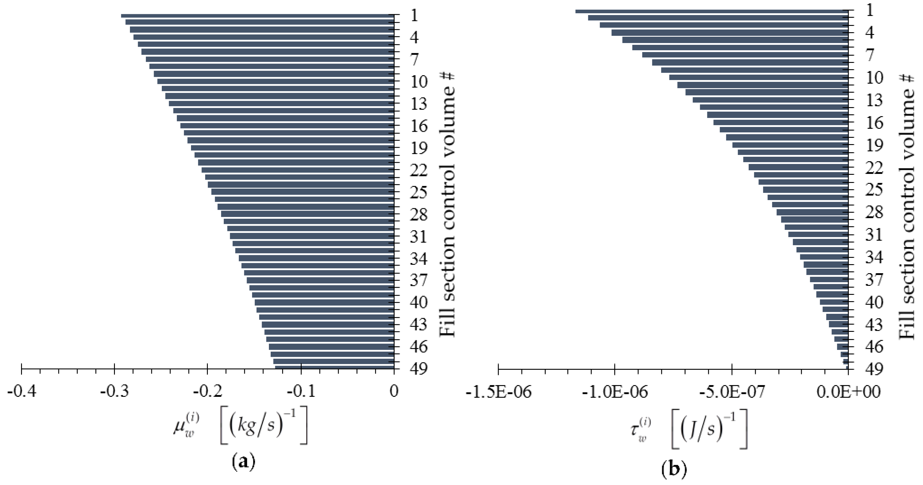
2.2.2. Verification of the Adjoint Functions for the Outlet Water Temperature Response $T_w^{(50)}$

When $R=T_w^{(50)}$, the quantities $r_{\ell }^{\left(i\right)}$ defined in Equation (25) all vanish except for a single component, namely: $r_2^{\left(49\right)}\triangleq \partial R/\partial T_w^{\left(50\right)}=1.$ Thus, the adjoint functions corresponding to the outlet water temperature response $T_w^{(50)}$ are computed by solving the adjoint sensitivity system given in Equation (28) using $r_2^{\left(49\right)}\triangleq \partial R/\partial T_w^{\left(50\right)}=1..$ as the only non-zero source term; for this case, the solution of Equation (28) has been depicted in Figure 9.

(a) Verification of the adjoint function $o^{\left(49\right)}$

Note that the value of the adjoint function $o^{\left(49\right)}$ obtained by solving the adjoint sensitivity system given in Equation (28) is $o^{\left(49\right)}=-2.214\times {10}^{-4}\left[K/\left(J/kg\right)\right]$, as indicated in Figure 9. Now select a variation $\delta T_{a,in}$ in the inlet air temperature $T_{a,in}$, and note that Equation (40) yields the following expression for the sensitivity of the response $R=T_w^{(50)}$ to $T_{a,in}$:

$$\begin{array}{ll}{S}_{46}& \triangleq \frac{\partial T_w^{(50)}}{\partial T_{a,in}}-{\displaystyle \sum _{i=1}^{49}\left({\mu }_w^{\left(i\right)}\frac{\partial N_1^{\left(i\right)}}{\partial T_{a,in}}+{\tau }_w^{\left(i\right)}\frac{\partial N_2^{\left(i\right)}}{\partial T_{a,in}}+{\tau }_a^{\left(i\right)}\frac{\partial N_3^{\left(i\right)}}{\partial T_{a,in}}+o^{\left(i\right)}\frac{\partial N_4^{\left(i\right)}}{\partial T_{a,in}}\right)}=0-o^{\left(49\right)}\frac{\partial N_4^{\left(49\right)}}{\partial T_{a,in}}\\ & =-(o^{\left(49\right)})\left[C_p(\frac{T_a^{(49)}+tK}{2},\mathit{\alpha })+{\omega }_{in}{\alpha }_{1g}\right].\end{array}$$

(52)

Re-writing Equation (52) in the form:

$$o^{\left(49\right)}=-\frac{S_{46}}{\partial N_4^{\left(49\right)}/\partial T_{a,in}}=-S_{46}{\left[C_p(\frac{T_a^{(49)}+tK}{2},)+{\omega }_{in}{\alpha }_{1g}\right]}^{-1}$$

(53)

indicates that the value of the adjoint function $o^{\left(49\right)}$ could be computed independently if the sensitivity $S_{46}$ were available, since the quantity $\partial N_4^{\left(49\right)}/\partial T_{a,in}=1.0309\times {10}^3\left[J/\left(kg\cdot K\right)\right]$ is known. To first-order in the parameter perturbation, the finite-difference formula given in Equation (41) can be used to compute the approximate sensitivity $S_{46}^{FD}$; subsequently, this value can be used in conjunction with Equation (53) to compute a “finite-difference sensitivity” value, denoted as ${\left[o^{\left(49\right)}\right]}^{SFD}$, for the respective adjoint, which would be accurate up to second-order in the respective parameter perturbation:

$${\left[o^{\left(49\right)}\right]}^{SFD}=-\frac{S_{46}^{FD}}{\partial N_4^{\left(49\right)}/\partial T_{a,in}}=-\left[\frac{T_{w,pert}^{(50)}-T_{w,nom}^{(50)}}{\delta T_{a,in}}\right]{\left[\frac{\partial N_4^{\left(49\right)}}{\partial T_{a,in}}\right]}^{-1}.$$

(54)

Numerically, the inlet air temperature $T_{a,in}(=T_{db})$ has the nominal (“base-case”) value of $T_{a,in}^0=299.11\left[K\right]$. The corresponding nominal value $T_{w,nom}^{(50)}$ of the response $T_w^{(50)}$ is $T_{w,nom}^{(50)}=294.579\left[K\right]$. Consider next a perturbation $\delta T_{a,in}=\left(0.001\right)T_{a,in}^0$, for which the perturbed value of the inlet air temperature becomes $T_{a,in}^{pert}=T_{a,in}^0+\delta T_{a,in}=299.40911\left[K\right]$. Re-computing the perturbed response by solving Equations (2)–(13) with the value of $T_{a,in}^{pert}$ yields the “perturbed response” value $T_{w,pert}^{(50)}=294.645\left[K\right]$. Using now the nominal and perturbed response values together with the parameter perturbation in the finite-difference expression given in Equation (41) yields the corresponding “finite-difference-computed sensitivity” $S_{46}^{FD}\triangleq \frac{T_{w,pert}^{(50)}-T_{w,nom}^{(50)}}{\delta T_{a,in}}=0.2207$. Using this value together with the nominal values of the other quantities appearing in the expression on the right side of Equation (54) yields ${\left[o^{\left(49\right)}\right]}^{SFD}=-2.141\times {10}^{-4}\left[K/\left(J/kg\right)\right]$. This result compares well with the value $o^{\left(49\right)}=-2.214\times {10}^{-4}\left[K/\left(J/kg\right)\right]$ obtained by solving the adjoint sensitivity system given in Equation (28), cf., Figure 9. When solving this adjoint sensitivity system, the computation of $o^{\left(49\right)}$ depends on the previously computed adjoint functions $o^{\left(i\right)},i=1,\dots ,I-1$; hence, the forgoing verification of the computational accuracy of $o^{\left(49\right)}$ also provides an indirect verification that the functions $o^{\left(i\right)},i=1,\dots ,I-1,$ were also computed accurately.

(b) Verification of the adjoint function ${\tau }_a^{\left(49\right)}$

Note that the value of the adjoint function ${\tau }_a^{\left(49\right)}$ obtained by solving the adjoint sensitivity system given in Equation (28) is ${\tau }_a^{\left(49\right)}=-76.12\left[K\right]$, as indicated in Figure 9. Now select a variation $\delta {\omega }_{in}$ in the inlet air humidity ratio ${\omega }_{in}$, and note that Equation (40) yields the following expression for the sensitivity of the response $R=T_w^{(50)}$ to ${\omega }_{in}$:

$$\begin{array}{ll}{S}_{48}& \triangleq \frac{\partial T_w^{(50)}}{\partial {\omega }_{in}}-{\displaystyle \sum _{i=1}^{49}\left({\mu }_w^{\left(i\right)}\frac{\partial N_1^{\left(i\right)}}{\partial {\omega }_{in}}+{\tau }_w^{\left(i\right)}\frac{\partial N_2^{\left(i\right)}}{\partial {\omega }_{in}}+{\tau }_a^{\left(i\right)}\frac{\partial N_3^{\left(i\right)}}{\partial {\omega }_{in}}+o^{\left(i\right)}\frac{\partial N_4^{\left(i\right)}}{\partial {\omega }_{in}}\right)}\\ & =0-\left({\tau }_a^{\left(49\right)}\frac{\partial N_3^{\left(49\right)}}{\partial {\omega }_{in}}+o^{\left(49\right)}\frac{\partial N_4^{\left(49\right)}}{\partial {\omega }_{in}}\right)=-\left[{\tau }_a^{\left(49\right)}+o^{\left(49\right)}\cdot h_{g,a}^{(50)}(T_{a,in},\mathit{\alpha })\right].\end{array}$$

(55)

Re-writing Equation (55) in the form

$${\tau }_a^{\left(49\right)}=-S_{48}-o^{\left(49\right)}\cdot h_{g,a}^{(50)}\left(T_{a,in},\mathit{\alpha }\right)$$

(56)

indicates that the value of the adjoint function ${\tau }_a^{\left(49\right)}$ could be computed independently if the sensitivity $S_{48}$ were available, since the $o^{\left(49\right)}$ has been verified in (the previous) Section 2.2.2 (a) and the quantity $h_{g,a}^{(50)}\left(T_{a,in},\mathit{\alpha }\right)$ is known. To first-order in the parameter perturbation, the finite-difference formula given in Equation (41) can be used to compute the approximate sensitivity $S_{48}^{FD}$; subsequently, this value can be used in conjunction with Equation (56) to compute a “finite-difference sensitivity” value, denoted as ${\left[{\tau }_a^{\left(49\right)}\right]}^{SFD}$, for the respective adjoint, which would be accurate up to second-order in the respective parameter perturbation:

$${\left[{\tau }_a^{\left(49\right)}\right]}^{SFD}=-S_{48}^{FD}-o^{\left(49\right)}\cdot h_{g,a}^{(50)}\left(T_{a,in},\mathit{\alpha }\right)$$

(57)

Numerically, the inlet air humidity ratio ${\omega }_{in}$ has the nominal (“base-case”) value of ${\omega }_{in}^0=0.0137746$. The corresponding nominal value $T_{w,nom}^{(50)}$ of the response $T_w^{(50)}$ is $T_{w,nom}^{(50)}=294.579029\left[K\right]$. Consider next a perturbation $\delta {\omega }_{in}=\left(0.0063\right){\omega }_{in}^0$, for which the perturbed value of the inlet air humidity ratio becomes ${\omega }_{in}^{pert}={\omega }_{in}^0+\delta {\omega }_{in}=0.0138612$. Re-computing the perturbed response by solving Equations (2)–(13) with the value of ${\omega }_{in}^{pert}$ yields the “perturbed response” value $T_{w,pert}^{(50)}=294.634438\left[K\right]$. Using now the nominal and perturbed response values together with the parameter perturbation in the finite-difference expression given in Equation (41) yields the corresponding “finite-difference-computed sensitivity” $S_{48}^{FD}\triangleq \frac{T_{w,pert}^{(50)}-T_{w,nom}^{(50)}}{\delta {\omega }_{in}}=639.98\left[K\right]$. Using this value together with the nominal values of the other quantities appearing in the expression on the right side of Equation (57) yields ${\left[{\tau }_a^{\left(49\right)}\right]}^{SFD}=-75.64\left[K\right]$. This result compares well with the value ${\tau }_a^{\left(49\right)}=-76.12\left[K\right]$ obtained by solving the adjoint sensitivity system given in Equation (28), cf. Figure 9. When solving this adjoint sensitivity system, the computation of ${\tau }_a^{\left(49\right)}$ depends on the previously computed adjoint functions ${\tau }_a^{\left(i\right)},i=1,\dots ,I-1$; hence, the forgoing verification of the computational accuracy of ${\tau }_a^{\left(49\right)}$ also provides an indirect verification that the functions ${\tau }_a^{\left(i\right)},i=1,\dots ,I-1$ were also computed accurately.

(c) Verification of the adjoint functions ${\tau }_w^{\left(1\right)}$ and ${\mu }_w^{\left(1\right)}$

Note that the values of the adjoint functions ${\tau }_w^{\left(1\right)}$ and ${\mu }_w^{\left(1\right)}$ obtained by solving the adjoint sensitivity system given in Equation (28) are as follows: ${\tau }_w^{\left(1\right)}=-5.730\times {10}^{-7}\left[K/(J/s)\right]$ and ${\mu }_w^{\left(1\right)}=1.3996\left[K/\left(kg/s\right)\right]$, respectively, as indicated in Figure 9. Now select a variation $\delta T_{w,in}$ in the inlet water temperature $T_{w,in}$, and note that Equation (40) yields the following expression for the sensitivity of the response $R=T_w^{(50)}$ to $T_{w,in}$:

$$\begin{array}{ll}{S}_3& \triangleq \frac{\partial T_w^{(50)}}{\partial T_{w,in}}-{\displaystyle \sum _{i=1}^{49}\left({\mu }_w^{\left(i\right)}\frac{\partial N_1^{\left(i\right)}}{\partial T_{w,in}}+{\tau }_w^{\left(i\right)}\frac{\partial N_2^{\left(i\right)}}{\partial T_{w,in}}+{\tau }_a^{\left(i\right)}\frac{\partial N_3^{\left(i\right)}}{\partial T_{w,in}}+o^{\left(i\right)}\frac{\partial N_4^{\left(i\right)}}{\partial T_{w,in}}\right)}\\ & =0-\left({\mu }_w^{\left(1\right)}\frac{\partial N_1^{\left(1\right)}}{\partial T_{w,in}}+{\tau }_w^{\left(1\right)}\frac{\partial N_2^{\left(1\right)}}{\partial T_{w,in}}+{\tau }_a^{\left(1\right)}\frac{\partial N_3^{\left(1\right)}}{\partial T_{w,in}}+o^{\left(1\right)}\frac{\partial N_4^{\left(1\right)}}{\partial T_{w,in}}\right).\end{array}$$

(58)

Since the adjoint functions ${\tau }_a^{\left(49\right)}$ and $o^{\left(49\right)}$ have been already verified as described in Section 2.2.2 (a) and (b), it follows that the computed values of adjoint functions ${\tau }_a^{\left(1\right)}=-0.88745\left[K\right]$ $o^{\left(1\right)}=-1.38335\times {10}^{-6}\left[K/\left(J/kg\right)\right]$ can also be considered as being accurate, since they constitute the starting point for solving the adjoint sensitivity system in Equation (28). Hence, the unknowns in Equation (58) are the adjoint functions ${\mu }_w^{\left(1\right)}$ and ${\tau }_w^{\left(1\right)}$. A second equation involving solely these adjoint functions can be derived by selecting a perturbation, $\delta m_{w,in}$, in the inlet water mass flow rate, $m_{w,in}$, for which Equation (40) yields the following expression for the sensitivity of the response $R=T_w^{(50)}$ to $m_{w,in}$:

$$\begin{array}{ll}{S}_{45}& \triangleq \frac{\partial T_w^{(50)}}{\partial m_{w,in}}-{\displaystyle \sum _{i=1}^{49}\left({\mu }_w^{\left(i\right)}\frac{\partial N_1^{\left(i\right)}}{\partial m_{w,in}}+{\tau }_w^{\left(i\right)}\frac{\partial N_2^{\left(i\right)}}{\partial m_{w,in}}+{\tau }_a^{\left(i\right)}\frac{\partial N_3^{\left(i\right)}}{\partial m_{w,in}}+o^{\left(i\right)}\frac{\partial N_4^{\left(i\right)}}{\partial m_{w,in}}\right)}\\ & =0-\left({\mu }_w^{\left(1\right)}\frac{\partial N_1^{\left(1\right)}}{\partial m_{w,in}}+{\tau }_w^{\left(1\right)}\frac{\partial N_2^{\left(1\right)}}{\partial m_{w,in}}+{\tau }_a^{\left(1\right)}\frac{\partial N_3^{\left(1\right)}}{\partial m_{w,in}}+o^{\left(1\right)}\frac{\partial N_4^{\left(1\right)}}{\partial m_{w,in}}\right).\end{array}$$

(59)

Numerically, the inlet water temperature, $T_{w,in}$, has the nominal (“base-case”) value of $T_{w,in}^0=298.79\left[K\right]$, while the nominal (“base-case”) value of the inlet water mass flow rate is $m_{w,in}^0=44.021229\left[kg/s\right]$. As before, the corresponding nominal value $T_{w,nom}^{(50)}$ of the response $T_w^{(50)}$ is $T_{w,nom}^{(50)}=294.579\left[K\right]$. Consider now a perturbation $\delta T_{w,in}=\left(0.00033\right)T_{w,in}^0$, for which the perturbed value of the inlet air temperature becomes $T_{w,in}^{pert}=T_{w,in}^0+\delta T_{w,in}=298.89\left[K\right]$. Re-computing the perturbed response by solving Equations (2)–(13) with the value of $T_{w,in}^{pert}$ yields the “perturbed response” value $T_{w,pert}^{(50)}=294.5895\left[K\right]$. Using now the nominal and perturbed response values together with the parameter perturbation in the finite-difference expression given in Equation (41) yields the corresponding “finite-difference-computed sensitivity” $S_3^{FD}\triangleq \frac{T_{w,pert}^{(50)}-T_{w,nom}^{(50)}}{\delta T_{w,in}}=0.1049$.

Next, consider a perturbation $\delta m_{w,in}=\left(0.001\right)m_{w,in}^0$, for which the perturbed value of the inlet air temperature becomes $m_{w,in}^{pert}=m_{w,in}^0+\delta m_{w,in}=44.065252\left[kg/s\right]$. Re-computing the perturbed response by solving Equations (2)–(13) with the value of $m_{w,in}^{pert}$ yields the “perturbed response” value $T_{w,pert}^{(50)}=294.5804\left[K\right]$. Using now the nominal and perturbed response values together with the parameter perturbation in the finite-difference expression given in Equation (41) yields the corresponding “finite-difference-computed sensitivity” $S_{45}^{FD}\triangleq \frac{T_{w,pert}^{(50)}-T_{w,nom}^{(50)}}{\delta m_{w,in}}=0.02986$. Inserting now all of the numerical values of the known quantities in Equations (58) and (59) yields the following system of coupled equations for obtaining ${\mu }_w^{\left(1\right)}$ and ${\tau }_w^{\left(1\right)}$:

$$0.1049=-\left[\left(0.0161\right){\mu }_w^{\left(1\right)}+\left(223597\right){\tau }_w^{\left(1\right)}+\left(-0.88745\right)\cdot \left(-1.039\times {10}^{-4}\right)+\left(-1.38335\times {10}^{-6}\right)\cdot \left(-264.65\right)\right]$$

(60)

$$0.02986=-\left[-{\mu }_w^{\left(1\right)}+\left(-2.44038\times {10}^6\right){\tau }_w^{\left(1\right)}+\left(-0.88745\right)\cdot \left(0.0064\right)+\left(-1.38335\times {10}^{-6}\right)\cdot \left(16430.26\right)\right]$$

(61)

Solving Equations (60) and (61) yields ${\mu }_w^{\left(1\right)}=1.3969\left[K/\left(kg/s\right)\right]$ and ${\tau }_w^{\left(1\right)}=-5.718\times {10}^{-7}\left[K/(J/s)\right]$. These values compare well with the values ${\mu }_w^{\left(1\right)}=1.3996\left[K/\left(kg/s\right)\right]$ and ${\tau }_w^{\left(1\right)}=-5.730\times {10}^{-7}\left[K/(J/s)\right]$, respectively, which are obtained by solving the adjoint sensitivity system given in Equation (28), cf. Figure 9.

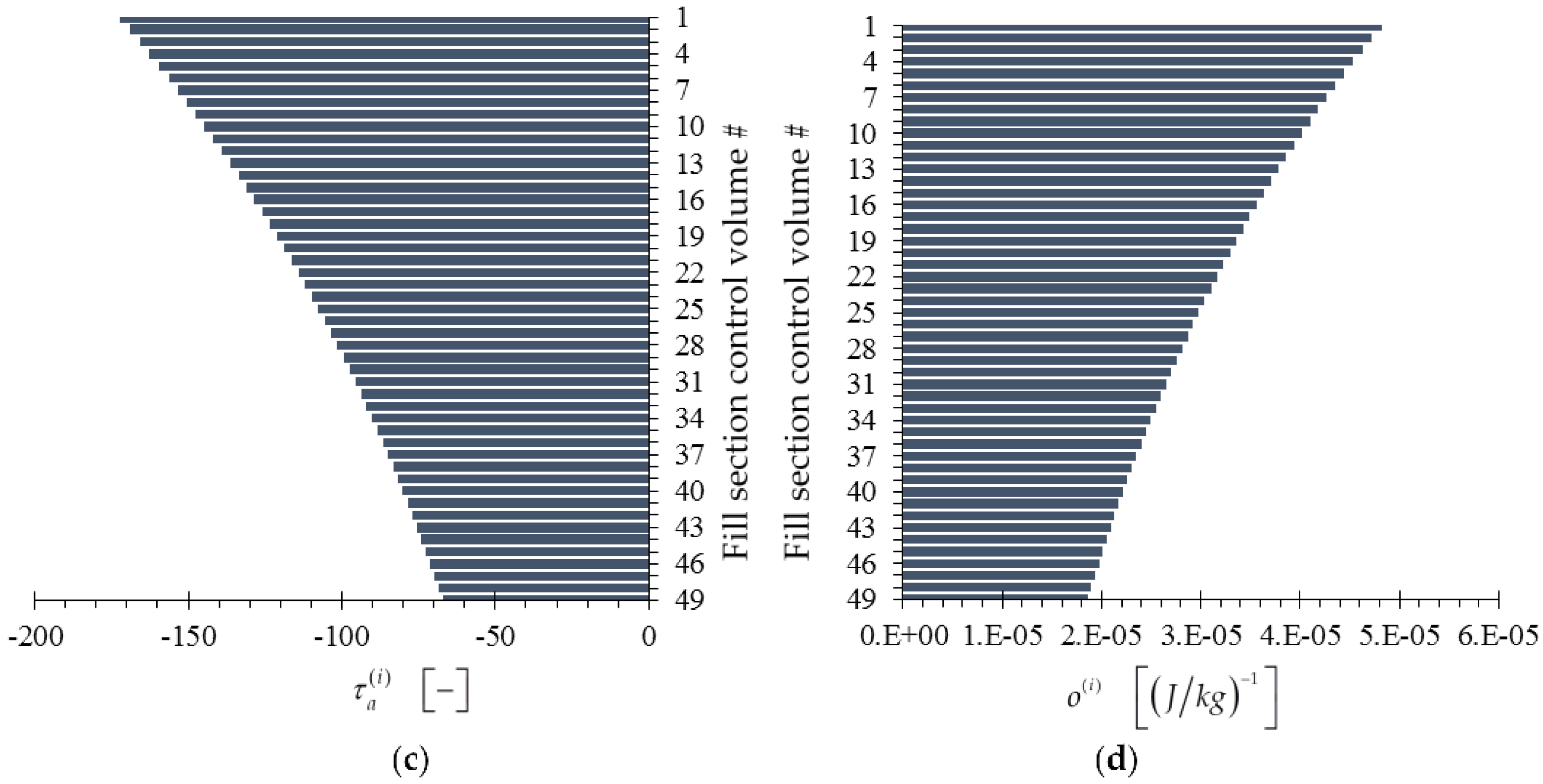
2.2.3. Verification of the Adjoint Functions for the Outlet Air Relative Humidity Response $R{H}^{(1)}$

When $R=R{H}^{(1)}$, the quantities $r_{\ell }^{\left(i\right)}$ defined in Equation (25) all vanish except for two components, namely:

$$r_3^{\left(1\right)}\triangleq \frac{\partial \left(R{H}^{(1)}\right)}{\partial T_a^{\left(1\right)}}=\frac{\partial }{\partial T_a^{(1)}}\left[\frac{P_v\left({\mathsf{\omega }}^{(1)},\mathit{\alpha }\right)}{P_{vs}\left(T_a^{(1)},\mathit{\alpha }\right)}\times 100\right]=\frac{0.622P_{atm}}{\left(0.622+{\omega }^{\left(1\right)}\right)e^{a_0+\frac{a_1}{T_a^{(1)}}}}\frac{a_1}{{\left[T_a^{(1)}\right]}^2}\times 100;$$

(62)

$$r_4^{\left(1\right)}\triangleq \frac{\partial \left(R{H}^{(1)}\right)}{\partial {\omega }^{\left(1\right)}}=\frac{\partial }{\partial {\omega }^{\left(1\right)}}\left[\frac{P_v\left({\mathsf{\omega }}^{(1)},\mathit{\alpha }\right)}{P_{vs}\left(T_a^{(1)},\mathit{\alpha }\right)}\times 100\right]=\frac{0.622P_{atm}}{{\left(0.622+{\omega }^{\left(1\right)}\right)}^2{e}^{a_0+\frac{a_1}{T_a^{(1)}}}}\times 100.$$

(63)

Thus, the adjoint functions corresponding to the outlet air relative humidity response $R{H}^{(1)}$ are computed by solving the adjoint sensitivity system given in Equation (28) using $r_3^{\left(1\right)}$ and $r_4^{\left(1\right)}$ as the only two non-zero source terms; for this case, the solution of Equation (28) has been depicted in Figure 10.

(a) Verification of the adjoint function $o^{\left(49\right)}$

Note that the value of the adjoint function $o^{\left(49\right)}$ obtained by solving the adjoint sensitivity system given in Equation (28) is $o^{\left(49\right)}=1.860\times {10}^{-5}\left[{\left(J/kg\right)}^{-1}\right]$, as indicated in Figure 10. Now select a variation $\delta T_{a,in}$ in the inlet air temperature $T_{a,in}$, and note that Equation (40) yields the following expression for the sensitivity of the response $R=R{H}^{(1)}$ to $T_{a,in}$:

$$\begin{array}{ll}{S}_{46}& \triangleq \frac{\partial R{H}^{(1)}}{\partial T_{a,in}}-{\displaystyle \sum _{i=1}^{49}\left({\mu }_w^{\left(i\right)}\frac{\partial N_1^{\left(i\right)}}{\partial T_{a,in}}+{\tau }_w^{\left(i\right)}\frac{\partial N_2^{\left(i\right)}}{\partial T_{a,in}}+{\tau }_a^{\left(i\right)}\frac{\partial N_3^{\left(i\right)}}{\partial T_{a,in}}+o^{\left(i\right)}\frac{\partial N_4^{\left(i\right)}}{\partial T_{a,in}}\right)}=0-o^{\left(49\right)}\frac{\partial N_4^{\left(49\right)}}{\partial T_{a,in}}\\ & =-(o^{\left(49\right)})\left[C_p(\frac{T_a^{(49)}+tK}{2},\mathit{\alpha })+{\omega }_{in}{\alpha }_{1g}\right].\end{array}$$

(64)

Re-writing Equation (64) in the form:

$$o^{\left(49\right)}=-\frac{S_{46}}{\partial N_4^{\left(49\right)}/\partial T_{a,in}}=-S_{46}{\left[C_p(\frac{T_a^{(49)}+tK}{2},\mathit{\alpha })+{\omega }_{in}{\alpha }_{1g}\right]}^{-1}$$

(65)

indicates that the value of the adjoint function $o^{\left(49\right)}$ could be computed independently if the sensitivity $S_{46}$ were available, since the quantity $\partial N_4^{\left(49\right)}/\partial T_{a,in}=1.0309\times {10}^3\left[J/\left(kg\cdot K\right)\right]$ is known. To first-order in the parameter perturbation, the finite-difference formula given in Equation (41) can be used to compute the approximate sensitivity $S_{46}^{FD}$; subsequently, this value can be used in conjunction with Equation (65) to compute a “finite-difference sensitivity” value, denoted as ${\left[o^{\left(49\right)}\right]}^{SFD}$, for the respective adjoint, which would be accurate up to second-order in the parameter perturbation:

$${\left[o^{\left(49\right)}\right]}^{SFD}=-\frac{S_{46}^{FD}}{\partial N_4^{\left(49\right)}/\partial T_{a,in}}=-\left[\frac{R{H}_{pert}^{(1)}-R{H}_{nom}^{(1)}}{\delta T_{a,in}}\right]{\left[\frac{\partial N_4^{\left(49\right)}}{\partial T_{a,in}}\right]}^{-1}$$

(66)

Numerically, the inlet air temperature $T_{a,in}(=T_{db})$ has the nominal (“base-case”) value of $T_{a,in}^0=299.11\left[K\right]$. The corresponding nominal value $R{H}_{nom}^{(1)}$ of the response $R{H}^{(1)}$ is $R{H}_{nom}^{(1)}=86.11678\%$. Consider next a perturbation $\delta T_{a,in}=\left(0.001\right)T_{a,in}^0$, for which the perturbed value of the inlet air temperature becomes $T_{a,in}^{pert}=T_{a,in}^0+\delta T_{a,in}=299.40911\left[K\right]$. Re-computing the perturbed response by solving Equations (2)–(13) with the value of $T_{a,in}^{pert}$ yields the “perturbed response” value $R{H}_{pert}^{(1)}=85.55717\%$. Using now the nominal and perturbed response values together with the parameter perturbation in the finite-difference expression given in Equation (41) yields the corresponding “finite-difference-computed sensitivity” $S_{46}^{FD}\triangleq \frac{R{H}_{pert}^{(1)}-R{H}_{nom}^{(1)}}{\delta T_{a,in}}=-0.018709\left[\frac{1}{K}\right]$. Using this value together with the nominal values of the other quantities appearing in the expression on the right side of Equation (66) yields ${\left[o^{\left(49\right)}\right]}^{SFD}=1.815\times {10}^{-5}\left[{\left(J/kg\right)}^{-1}\right]$. This result compares well with the value $o^{\left(49\right)}=1.860\times {10}^{-5}\left[{\left(J/kg\right)}^{-1}\right]$ obtained by solving the adjoint sensitivity system given in Equation (28), cf., Figure 10. When solving this adjoint sensitivity system, the computation of $o^{\left(49\right)}$ depends on the previously computed adjoint functions $o^{\left(i\right)},i=1,\dots ,I-1$; hence, the forgoing verification of the computational accuracy of $o^{\left(49\right)}$ also provides an indirect verification that the functions $o^{\left(i\right)},i=1,\dots ,I-1,$ were also computed accurately.

(b) Verification of the adjoint function ${\tau }_a^{\left(49\right)}$

Note that the value of the adjoint function ${\tau }_a^{\left(49\right)}$ obtained by solving the adjoint sensitivity system given in Equation (28) is ${\tau }_a^{\left(49\right)}=-67.047$, as indicated in Figure 10. Now select a variation $\delta {\omega }_{in}$ in the inlet air humidity ratio ${\omega }_{in}$, and note that Equation (40) yields the following expression for the sensitivity of the response $R=R{H}^{(1)}$ to ${\omega }_{in}$:

$$\begin{array}{ll}{S}_{48}& \triangleq \frac{\partial R{H}^{(1)}}{\partial {\omega }_{in}}-{\displaystyle \sum _{i=1}^{49}\left({\mu }_w^{\left(i\right)}\frac{\partial N_1^{\left(i\right)}}{\partial {\omega }_{in}}+{\tau }_w^{\left(i\right)}\frac{\partial N_2^{\left(i\right)}}{\partial {\omega }_{in}}+{\tau }_a^{\left(i\right)}\frac{\partial N_3^{\left(i\right)}}{\partial {\omega }_{in}}+o^{\left(i\right)}\frac{\partial N_4^{\left(i\right)}}{\partial {\omega }_{in}}\right)}\\ & =0-\left({\tau }_a^{\left(49\right)}\frac{\partial N_3^{\left(49\right)}}{\partial {\omega }_{in}}+o^{\left(49\right)}\frac{\partial N_4^{\left(49\right)}}{\partial {\omega }_{in}}\right)=-\left[{\tau }_a^{\left(49\right)}+o^{\left(49\right)}\cdot h_{g,a}^{(50)}(T_{a,in},\mathit{\alpha })\right].\end{array}$$

(67)

Re-writing Equation (67) in the form

$${\tau }_a^{\left(49\right)}=-S_{48}-o^{\left(49\right)}\cdot h_{g,a}^{(50)}\left(T_{a,in},\mathit{\alpha }\right)$$

(68)

indicates that the value of the adjoint function ${\tau }_a^{\left(49\right)}$ could be computed independently if the sensitivity $S_{48}$ were available, since the $o^{\left(49\right)}$ has been verified in (the previous) Section 2.2.3 (a) and the quantity $h_{g,a}^{(50)}\left(T_{a,in},\mathit{\alpha }\right)$ is known. To first-order in the parameter perturbation, the finite-difference formula given in Equation (41) can be used to compute the approximate sensitivity $S_{48}^{FD}$; subsequently, this value can be used in conjunction with Equation (68) to compute a “finite-difference sensitivity” value, denoted as ${\left[{\tau }_a^{\left(49\right)}\right]}^{SFD}$, for the respective adjoint, which would be accurate up to second-order in the parameter perturbation:

$${\left[{\tau }_a^{\left(49\right)}\right]}^{SFD}=-S_{48}^{FD}-o^{\left(49\right)}\cdot h_{g,a}^{(50)}\left(T_{a,in},\mathit{\alpha }\right)$$

(69)

Numerically, the inlet air humidity ratio ${\omega }_{in}$ has the nominal (“base-case”) value of ${\omega }_{in}^0=0.0137746$. The corresponding nominal value $R{H}_{nom}^{(1)}$ of the response $R{H}^{(1)}$ is $R{H}_{nom}^{(1)}=86.11678\%$. Consider next a perturbation $\delta {\omega }_{in}=\left(0.0063\right){\omega }_{in}^0$, for which the perturbed value of the inlet air humidity ratio becomes ${\omega }_{in}^{pert}={\omega }_{in}^0+\delta {\omega }_{in}=0.0138612$. Re-computing the perturbed response by solving Equations (2)–(13) with the value of ${\omega }_{in}^{pert}$ yields the “perturbed response” value $R{H}_{pert}^{(1)}=86.28967\%$. Using now the nominal and perturbed response values together with the parameter perturbation in the finite-difference expression given in Equation (41) yields the corresponding “finite-difference-computed sensitivity” $S_{48}^{FD}\triangleq \frac{R{H}_{pert}^{(1)}-R{H}_{nom}^{(1)}}{\delta {\omega }_{in}}=19.6252$. Using this value together with the nominal values of the other quantities appearing in the expression on the right side of Equation (69) yields ${\left[{\tau }_a^{\left(49\right)}\right]}^{SFD}=-67.034$. This result compares well with the value ${\tau }_a^{\left(49\right)}=-67.047$ obtained by solving the adjoint sensitivity system given in Equation (28), cf. Figure 10. When solving this adjoint sensitivity system, the computation of ${\tau }_a^{\left(49\right)}$ depends on the previously computed adjoint functions ${\tau }_a^{\left(i\right)},i=1,\dots ,I-1$; hence, the forgoing verification of the computational accuracy of ${\tau }_a^{\left(49\right)}$ also provides an indirect verification that the functions ${\tau }_a^{\left(i\right)},i=1,\dots ,I-1$ were also computed accurately.

(c) Verification of the adjoint functions ${\tau }_w^{\left(1\right)}$ and ${\mu }_w^{\left(1\right)}$

Note that the values of the adjoint functions ${\tau }_w^{\left(1\right)}$ and ${\mu }_w^{\left(1\right)}$ obtained by solving the adjoint sensitivity system given in Equation (28) are as follows: ${\tau }_w^{\left(1\right)}=-1.168\times {10}^{-8}\left[({J/s)}^{-1}\right]$ and ${\mu }_w^{\left(1\right)}=-0.2926\left[{\left(kg/s\right)}^{-1}\right]$, respectively, as indicated in Figure 10. Now select a variation $\delta T_{w,in}$ in the inlet water temperature $T_{w,in}$, and note that Equation (40) yields the following expression for the sensitivity of the response $R=R{H}^{(1)}$ to $T_{w,in}$:

$$\begin{array}{ll}{S}_3& \triangleq \frac{\partial R{H}^{(1)}}{\partial T_{w,in}}-{\displaystyle \sum _{i=1}^{49}\left({\mu }_w^{\left(i\right)}\frac{\partial N_1^{\left(i\right)}}{\partial T_{w,in}}+{\tau }_w^{\left(i\right)}\frac{\partial N_2^{\left(i\right)}}{\partial T_{w,in}}+{\tau }_a^{\left(i\right)}\frac{\partial N_3^{\left(i\right)}}{\partial T_{w,in}}+o^{\left(i\right)}\frac{\partial N_4^{\left(i\right)}}{\partial T_{w,in}}\right)}\\ & =0-\left({\mu }_w^{\left(1\right)}\frac{\partial N_1^{\left(1\right)}}{\partial T_{w,in}}+{\tau }_w^{\left(1\right)}\frac{\partial N_2^{\left(1\right)}}{\partial T_{w,in}}+{\tau }_a^{\left(1\right)}\frac{\partial N_3^{\left(1\right)}}{\partial T_{w,in}}+o^{\left(1\right)}\frac{\partial N_4^{\left(1\right)}}{\partial T_{w,in}}\right).\end{array}$$

(70)

Since the adjoint functions ${\tau }_a^{\left(49\right)}$ and $o^{\left(49\right)}$ have been already verified as described in Section 2.2.3 (a) and (b), it follows that the computed values of adjoint functions ${\tau }_a^{\left(1\right)}=-172.515$ and $o^{\left(1\right)}=4.816\times {10}^{-5}\left[{\left(J/kg\right)}^{-1}\right]$ can also be considered as being accurate, since they constitute the starting point for solving the adjoint sensitivity system in Equation (28). Hence, the unknowns in Equation (70) are the adjoint functions ${\mu }_w^{\left(1\right)}$ and ${\tau }_w^{\left(1\right)}$. A second equation involving solely these adjoint functions can be derived by selecting a perturbation, $\delta m_{w,in}$, in the inlet water mass flow rate, $m_{w,in}$, for which Equation (40) yields the following expression for the sensitivity of the response $R=R{H}^{(1)}$ to $m_{w,in}$:

$$\begin{array}{ll}{S}_{45}& \triangleq \frac{\partial R{H}^{(1)}}{\partial m_{w,in}}-{\displaystyle \sum _{i=1}^{49}\left({\mu }_w^{\left(i\right)}\frac{\partial N_1^{\left(i\right)}}{\partial m_{w,in}}+{\tau }_w^{\left(i\right)}\frac{\partial N_2^{\left(i\right)}}{\partial m_{w,in}}+{\tau }_a^{\left(i\right)}\frac{\partial N_3^{\left(i\right)}}{\partial m_{w,in}}+o^{\left(i\right)}\frac{\partial N_4^{\left(i\right)}}{\partial m_{w,in}}\right)}\\ & =0-\left({\mu }_w^{\left(1\right)}\frac{\partial N_1^{\left(1\right)}}{\partial m_{w,in}}+{\tau }_w^{\left(1\right)}\frac{\partial N_2^{\left(1\right)}}{\partial m_{w,in}}+{\tau }_a^{\left(1\right)}\frac{\partial N_3^{\left(1\right)}}{\partial m_{w,in}}+o^{\left(1\right)}\frac{\partial N_4^{\left(1\right)}}{\partial m_{w,in}}\right).\end{array}$$

(71)

Numerically, the inlet water temperature, $T_{w,in}$, has the nominal (“base-case”) value of $T_{w,in}^0=298.79\left[K\right]$, while the nominal (“base-case”) value of the inlet water mass flow rate is $m_{w,in}^0=44.021229\left[kg/s\right]$. As before, the corresponding nominal value $R{H}_{nom}^{(1)}$ of the response $R{H}^{(1)}$ is $R{H}_{nom}^{(1)}=86.11678\%$. Consider now a perturbation $\delta T_{w,in}=\left(0.00033\right)T_{w,in}^0$, for which the perturbed value of the inlet air temperature becomes $T_{w,in}^{pert}=T_{w,in}^0+\delta T_{w,in}=298.89\left[K\right]$. Re-computing the perturbed response by solving Equations (2)–(13) with the value of $T_{w,in}^{pert}$ yields the “perturbed response” value $R{H}_{pert}^{(1)}=86.13838\%$. Using now the nominal and perturbed response values together with the parameter perturbation in the finite-difference expression given in Equation (41) yields the corresponding “finite-difference-computed sensitivity” $S_3^{FD}\triangleq \frac{R{H}_{pert}^{(1)}-R{H}_{nom}^{(1)}}{\delta T_{w,in}}=0.00216$.

Next, consider a perturbation $\delta m_{w,in}=\left(0.001\right)m_{w,in}^0$, for which the perturbed value of the inlet air temperature becomes $m_{w,in}^{pert}=m_{w,in}^0+\delta m_{w,in}=44.065252\left[kg/s\right]$. Re-computing the perturbed response by solving Equations (2)–(13) with the value of $m_{w,in}^{pert}$ yields the “perturbed response” value $R{H}_{pert}^{(1)}=86.11725\%$. Using now the nominal and perturbed response values together with the parameter perturbation in the finite-difference expression given in Equation (41) yields the corresponding “finite-difference-computed sensitivity” $S_{45}^{FD}\triangleq \frac{R{H}_{pert}^{(1)}-R{H}_{nom}^{(1)}}{\delta m_{w,in}}=0.000107$. Inserting now all of the numerical values of the known quantities in Equations (70) and (71) yields the following system of coupled equations for obtaining ${\mu }_w^{\left(1\right)}$ and ${\tau }_w^{\left(1\right)}$:

$$0.00216=-\left[\left(0.0161\right){\mu }_w^{\left(1\right)}+\left(223597\right){\tau }_w^{\left(1\right)}+\left(-172.52\right)\cdot \left(-1.039\times {10}^{-4}\right)+\left(4.816\times {10}^{-5}\right)\cdot \left(-264.65\right)\right]$$

(72)

$$0.000107=-\left[-{\mu }_w^{\left(1\right)}+\left(-2.44038\times {10}^6\right){\tau }_w^{\left(1\right)}+\left(-172.52\right)\left(0.0064\right)+\left(4.816\times {10}^{-5}\right)\left(16430.26\right)\right]$$

(73)

Solving Equations (72) and (73) yields ${\mu }_w^{\left(1\right)}=-0.2925\left[{\left(kg/s\right)}^{-1}\right]$ and ${\tau }_w^{\left(1\right)}=-1.173\times {10}^{-8}\left[({J/s)}^{-1}\right]$. These values compare well with the values ${\mu }_w^{\left(1\right)}=-0.2926\left[{\left(kg/s\right)}^{-1}\right]$ and ${\tau }_w^{\left(1\right)}=-1.168\times {10}^{-8}\left[({J/s)}^{-1}\right]$, respectively, which are obtained by solving the adjoint sensitivity system given in Equation (28), cf. Figure 10.

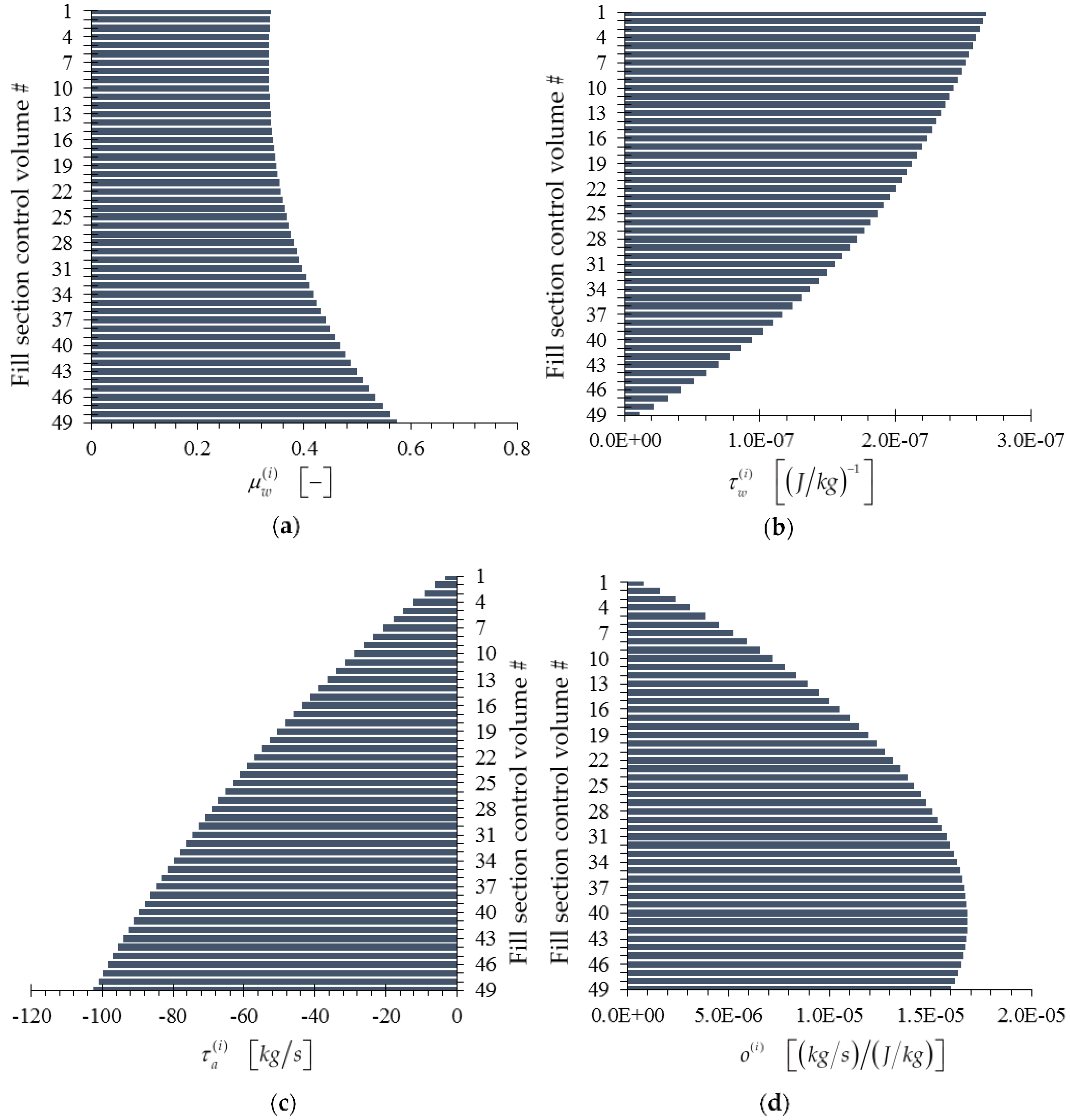
2.2.4. Verification of the Adjoint Functions for the Outlet Water Mass Flow Rate Response $m_w^{(50)}$

When $R=m_w^{(50)}$, the quantities $r_{\ell }^{\left(i\right)}$ defined in Equation (25) all vanish except for a single component, namely: $r_1^{\left(49\right)}\triangleq \partial R/\partial m_w^{\left(50\right)}=1.$Thus, the adjoint functions corresponding to the outlet water mass flow rate response $m_w^{(50)}$ are computed by solving the adjoint sensitivity system given in Equation (28) using $r_1^{\left(49\right)}\triangleq \partial R/\partial m_w^{\left(50\right)}=1.$ as the only non-zero source term; for this case, the solution of Equation (28) has been depicted in Figure 11.

(a) Verification of the adjoint function $o^{\left(49\right)}$

Note that the value of the adjoint function $o^{\left(49\right)}$ obtained by solving the adjoint sensitivity system given in Equation (28) is $o^{\left(49\right)}=1.603\times {10}^{-5}\left[\left(kg/s\right)/\left(J/kg\right)\right]$, as indicated in Figure 11. Now select a variation $\delta T_{a,in}$ in the inlet air temperature $T_{a,in}$, and note that Equation (40) yields the following expression for the sensitivity of the response $R=m_w^{(50)}$ to $T_{a,in}$:

$$\begin{array}{ll}{S}_{46}& \triangleq \frac{\partial m_w^{(50)}}{\partial T_{a,in}}-{\displaystyle \sum _{i=1}^{49}\left({\mu }_w^{\left(i\right)}\frac{\partial N_1^{\left(i\right)}}{\partial T_{a,in}}+{\tau }_w^{\left(i\right)}\frac{\partial N_2^{\left(i\right)}}{\partial T_{a,in}}+{\tau }_a^{\left(i\right)}\frac{\partial N_3^{\left(i\right)}}{\partial T_{a,in}}+o^{\left(i\right)}\frac{\partial N_4^{\left(i\right)}}{\partial T_{a,in}}\right)}=0-o^{\left(49\right)}\frac{\partial N_4^{\left(49\right)}}{\partial T_{a,in}}\\ & =-(o^{\left(49\right)})\left[C_p(\frac{T_a^{(49)}+tK}{2})+{\omega }_{in}{\alpha }_{1g}\right].\end{array}$$

(74)

Re-writing Equation (74) in the form:

$$o^{\left(49\right)}=-\frac{S_{46}}{\partial N_4^{\left(49\right)}/\partial T_{a,in}}=-S_{46}{\left[C_p(\frac{T_a^{(49)}+tK}{2})+{\omega }_{in}{\alpha }_{1g}\right]}^{-1}$$

(75)

indicates that the value of the adjoint function $o^{\left(49\right)}$ could be computed independently if the sensitivity $S_{46}$ were available, since the quantity $\partial N_4^{\left(49\right)}/\partial T_{a,in}=1.0309\times {10}^3\left[J/\left(kg\cdot K\right)\right]$ is known. To first-order in the parameter perturbation, the finite-difference formula given in Equation (41) can be used to compute the approximate sensitivity $S_{46}^{FD}$; subsequently, this value can be used in conjunction with Equation (75) to compute a “finite-difference sensitivity” value, denoted as ${\left[o^{\left(49\right)}\right]}^{SFD}$, for the respective adjoint, which would be accurate up to second-order in the parameter perturbation:

$${\left[o^{\left(49\right)}\right]}^{SFD}=-\frac{S_{46}^{FD}}{\partial N_4^{\left(49\right)}/\partial T_{a,in}}=-\left[\frac{m_{w,pert}^{(50)}-m_{w,nom}^{(50)}}{\delta T_{a,in}}\right]{\left[\frac{\partial N_4^{\left(49\right)}}{\partial T_{a,in}}\right]}^{-1}$$

(76)

Numerically, the inlet air temperature $T_{a,in}(=T_{db})$ has the nominal (“base-case”) value of $T_{a,in}^0=299.11\left[K\right]$. The corresponding nominal value $T_{w,nom}^{(50)}$ of the response $m_w^{(50)}$ is $m_{w,nom}^{(50)}=43.598097\left[kg/s\right]$. Consider next a perturbation $\delta T_{a,in}=\left(0.001\right)T_{a,in}^0$, for which the perturbed value of the inlet air temperature becomes $T_{a,in}^{pert}=T_{a,in}^0+\delta T_{a,in}=299.40911\left[K\right]$. Re-computing the perturbed response by solving Equations (2)–(13) with the value of $T_{a,in}^{pert}$ yields the “perturbed response” value $m_{w,pert}^{(50)}=43.59293\left[kg/s\right]$. Using now the nominal and perturbed response values together with the parameter perturbation in the finite-difference expression given in Equation (41) yields the corresponding “finite-difference-computed sensitivity” $S_{46}^{FD}\triangleq \frac{m_{w,pert}^{(50)}-m_{w,nom}^{(50)}}{\delta T_{a,in}}=-0.01728$. Using this value together with the nominal values of the other quantities appearing in the expression on the right side of Equation (76) yields ${\left[o^{\left(49\right)}\right]}^{SFD}=1.676\times {10}^{-5}\left[\left(kg/s\right)/\left(J/kg\right)\right]$. This result compares well with the value $o^{\left(49\right)}=1.603\times {10}^{-5}\left[\left(kg/s\right)/\left(J/kg\right)\right]$ obtained by solving the adjoint sensitivity system given in Equation (28), cf., Figure 11. When solving this adjoint sensitivity system, the computation of $o^{\left(49\right)}$ depends on the previously computed adjoint functions $o^{\left(i\right)},i=1,\dots ,I-1$; hence, the forgoing verification of the computational accuracy of $o^{\left(49\right)}$ also provides an indirect verification that the functions $o^{\left(i\right)},i=1,\dots ,I-1,$ were also computed accurately.

(b) Verification of the adjoint function ${\tau }_a^{\left(49\right)}$

Note that the value of the adjoint function ${\tau }_a^{\left(49\right)}$ obtained by solving the adjoint sensitivity system given in Equation (28) is ${\tau }_a^{\left(49\right)}=-102.42\left[kg/s\right]$, as indicated in Figure 11. Now select a variation $\delta {\omega }_{in}$ in the inlet air humidity ratio ${\omega }_{in}$, and note that Equation (40) yields the following expression for the sensitivity of the response $R=m_w^{(50)}$ to ${\omega }_{in}$:

$$\begin{array}{ll}{S}_{48}& \triangleq \frac{\partial m_w^{(50)}}{\partial {\omega }_{in}}-{\displaystyle \sum _{i=1}^{49}\left({\mu }_w^{\left(i\right)}\frac{\partial N_1^{\left(i\right)}}{\partial {\omega }_{in}}+{\tau }_w^{\left(i\right)}\frac{\partial N_2^{\left(i\right)}}{\partial {\omega }_{in}}+{\tau }_a^{\left(i\right)}\frac{\partial N_3^{\left(i\right)}}{\partial {\omega }_{in}}+o^{\left(i\right)}\frac{\partial N_4^{\left(i\right)}}{\partial {\omega }_{in}}\right)}\\ & =0-\left({\tau }_a^{\left(49\right)}\frac{\partial N_3^{\left(49\right)}}{\partial {\omega }_{in}}+o^{\left(49\right)}\frac{\partial N_4^{\left(49\right)}}{\partial {\omega }_{in}}\right)=-\left[{\tau }_a^{\left(49\right)}+o^{\left(49\right)}\cdot h_{g,a}^{(50)}(T_{a,in},\mathit{\alpha })\right].\end{array}$$

(77)

Re-writing Equation (77) in the form:

$${\tau }_a^{\left(49\right)}=-S_{48}-o^{\left(49\right)}\cdot h_{g,a}^{(50)}\left(T_{a,in},\mathit{\alpha }\right)$$

(78)

indicates that the value of the adjoint function ${\tau }_a^{\left(49\right)}$ could be computed independently if the sensitivity $S_{48}$ were available, since the $o^{\left(49\right)}$ has been verified in (the previous) Section 2.2.4 (a) and the quantity $h_{g,a}^{(50)}\left(T_{a,in},\mathsf{\alpha }\right)$ is known. To first-order in the parameter perturbation, the finite-difference formula given in Equation (41) can be used to compute the approximate sensitivity $S_{48}^{FD}$; subsequently, this value can be used in conjunction with Equation (78) to compute a “finite-difference sensitivity” value, denoted as ${\left[{\tau }_a^{\left(49\right)}\right]}^{SFD}$, for the respective adjoint, which would be accurate up to second-order in the parameter perturbation:

$${\left[{\tau }_a^{\left(49\right)}\right]}^{SFD}=-S_{48}^{FD}-o^{\left(49\right)}\cdot h_{g,a}^{(50)}\left(T_{a,in},\mathit{\alpha }\right)$$

(79)

Numerically, the inlet air humidity ratio ${\omega }_{in}$ has the nominal (“base-case”) value of ${\omega }_{in}^0=0.0137746$. The corresponding nominal value $m_{w,nom}^{(50)}$ of the response $m_w^{(50)}$ is $m_{w,nom}^{(50)}=43.598097\left[kg/s\right]$. Consider next a perturbation $\delta {\omega }_{in}=\left(0.0063\right){\omega }_{in}^0$, for which the perturbed value of the inlet air humidity ratio becomes ${\omega }_{in}^{pert}={\omega }_{in}^0+\delta {\omega }_{in}=0.0138612$. Re-computing the perturbed response by solving Equations (2)–(13) with the value of ${\omega }_{in}^{pert}$ yields the “perturbed response” value $m_{w,pert}^{(50)}=43.603424\left[kg/s\right]$. Using now the nominal and perturbed response values together with the parameter perturbation in the finite-difference expression given in Equation (41) yields the corresponding “finite-difference-computed sensitivity” $S_{48}^{FD}\triangleq \frac{m_{w,pert}^{(50)}-m_{w,nom}^{(50)}}{\delta {\omega }_{in}}=61.53\left[kg/s\right]$. Using this value together with the nominal values of the other quantities appearing in the expression on the right side of Equation (79) yields ${\left[{\tau }_a^{\left(49\right)}\right]}^{SFD}=-102.39\left[kg/s\right]$. This result compares well with the value ${\tau }_a^{\left(49\right)}=-102.42\left[kg/s\right]$ obtained by solving the adjoint sensitivity system given in Equation (28), cf. Figure 11. When solving this adjoint sensitivity system, the computation of ${\tau }_a^{\left(49\right)}$ depends on the previously computed adjoint functions ${\tau }_a^{\left(i\right)},i=1,\dots ,I-1$; hence, the forgoing verification of the computational accuracy of ${\tau }_a^{\left(49\right)}$ also provides an indirect verification that the functions ${\tau }_a^{\left(i\right)},i=1,\dots ,I-1$ were also computed accurately.

(c) Verification of the adjoint functions ${\tau }_w^{\left(1\right)}$ and ${\mu }_w^{\left(1\right)}$

Note that the values of the adjoint functions ${\tau }_w^{\left(1\right)}$ and ${\mu }_w^{\left(1\right)}$ obtained by solving the adjoint sensitivity system given in Equation (28) are as follows: ${\tau }_w^{\left(1\right)}=2.6710\times {10}^{-7}\left[{\left(J/kg\right)}^{-1}\right]$ and ${\mu }_w^{\left(1\right)}=0.3377$, respectively, as indicated in Figure 11. Now select a variation $\delta T_{w,in}$ in the inlet water temperature $T_{w,in}$, and note that Equation (40) yields the following expression for the sensitivity of the response $R=m_w^{(50)}$ to $T_{w,in}$:

$$\begin{array}{ll}{S}_3& \triangleq \frac{\partial m_w^{(50)}}{\partial T_{w,in}}-{\displaystyle \sum _{i=1}^{49}\left({\mu }_w^{\left(i\right)}\frac{\partial N_1^{\left(i\right)}}{\partial T_{w,in}}+{\tau }_w^{\left(i\right)}\frac{\partial N_2^{\left(i\right)}}{\partial T_{w,in}}+{\tau }_a^{\left(i\right)}\frac{\partial N_3^{\left(i\right)}}{\partial T_{w,in}}+o^{\left(i\right)}\frac{\partial N_4^{\left(i\right)}}{\partial T_{w,in}}\right)}\\ & =0-\left({\mu }_w^{\left(1\right)}\frac{\partial N_1^{\left(1\right)}}{\partial T_{w,in}}+{\tau }_w^{\left(1\right)}\frac{\partial N_2^{\left(1\right)}}{\partial T_{w,in}}+{\tau }_a^{\left(1\right)}\frac{\partial N_3^{\left(1\right)}}{\partial T_{w,in}}+o^{\left(1\right)}\frac{\partial N_4^{\left(1\right)}}{\partial T_{w,in}}\right).\end{array}$$

(80)

Since the adjoint functions ${\tau }_a^{\left(49\right)}$ and $o^{\left(49\right)}$ have been already verified as described in Section 2.2.4 (a) and (b), it follows that the computed values of adjoint functions ${\tau }_a^{\left(1\right)}=-3.1344\left[kg/s\right]$ $o^{\left(1\right)}=8.1328\times {10}^{-7}\left[\left(kg/s\right)/\left(J/kg\right)\right]$ can also be considered as being accurate, since they constitute the starting point for solving the adjoint sensitivity system in Equation (28). Hence, the unknowns in Equation (80) are the adjoint functions ${\mu }_w^{\left(1\right)}$ and ${\tau }_w^{\left(1\right)}$. A second equation involving solely these adjoint functions can be derived by selecting a perturbation, $\delta m_{w,in}$, in the inlet water mass flow rate, $m_{w,in}$, for which Equation (40) yields the following expression for the sensitivity of the response $R=m_w^{(50)}$ to $m_{w,in}$:

$$\begin{array}{ll}{S}_{45}& \triangleq \frac{\partial m_w^{(50)}}{\partial m_{w,in}}-{\displaystyle \sum _{i=1}^{49}\left({\mu }_w^{\left(i\right)}\frac{\partial N_1^{\left(i\right)}}{\partial m_{w,in}}+{\tau }_w^{\left(i\right)}\frac{\partial N_2^{\left(i\right)}}{\partial m_{w,in}}+{\tau }_a^{\left(i\right)}\frac{\partial N_3^{\left(i\right)}}{\partial m_{w,in}}+o^{\left(i\right)}\frac{\partial N_4^{\left(i\right)}}{\partial m_{w,in}}\right)}\\ & =0-\left({\mu }_w^{\left(1\right)}\frac{\partial N_1^{\left(1\right)}}{\partial m_{w,in}}+{\tau }_w^{\left(1\right)}\frac{\partial N_2^{\left(1\right)}}{\partial m_{w,in}}+{\tau }_a^{\left(1\right)}\frac{\partial N_3^{\left(1\right)}}{\partial m_{w,in}}+o^{\left(1\right)}\frac{\partial N_4^{\left(1\right)}}{\partial m_{w,in}}\right).\end{array}$$

(81)

Numerically, the inlet water temperature, $T_{w,in}$, has the nominal (“base-case”) value of $T_{w,in}^0=298.79\left[K\right]$, while the nominal (“base-case”) value of the inlet water mass flow rate is $m_{w,in}^0=44.021229\left[kg/s\right]$. As before, the corresponding nominal value $m_{w,nom}^{(50)}$ of the response $m_w^{(50)}$ is $m_{w,nom}^{(50)}=43.598097\left[kg/s\right]$. Consider now a perturbation $\delta T_{w,in}=\left(0.00033\right)T_{w,in}^0$, for which the perturbed value of the inlet air temperature becomes $T_{w,in}^{pert}=T_{w,in}^0+\delta T_{w,in}=298.89\left[K\right]$. Re-computing the perturbed response by solving Equations (2)–(13) with the value of $T_{w,in}^{pert}$ yields the “perturbed response” value $m_{w,pert}^{(50)}=43.591565\left[kg/s\right]$. Using now the nominal and perturbed response values together with the parameter perturbation in the finite-difference expression given in Equation (41) yields the corresponding “finite-difference-computed sensitivity” $S_3^{FD}\triangleq \frac{m_{w,pert}^{(50)}-m_{w,nom}^{(50)}}{\delta T_{w,in}}=-0.06531\left[\left(kg/s\right)/K\right]$.

Next, consider a perturbation $\delta m_{w,in}=\left(0.001\right)m_{w,in}^0$, for which the perturbed value of the inlet air temperature becomes $m_{w,in}^{pert}=m_{w,in}^0+\delta m_{w,in}=44.065252\left[kg/s\right]$. Re-computing the perturbed response by solving Equations (2)–(13) with the value of $m_{w,in}^{pert}$ yields the “perturbed response” value $m_{w,pert}^{(50)}=43.641962\left[kg/s\right]$. Using now the nominal and perturbed response values together with the parameter perturbation in the finite-difference expression given in Equation (41) yields the corresponding “finite-difference-computed sensitivity” $S_{45}^{FD}\triangleq \frac{m_{w,pert}^{(50)}-m_{w,nom}^{(50)}}{\delta m_{w,in}}=0.99646$. Inserting now all of the numerical values of the known quantities in Equations (80) and (81) yields the following system of coupled equations for obtaining ${\mu }_w^{\left(1\right)}$ and ${\tau }_w^{\left(1\right)}$:

$$-0.06531=-\left[\left(0.0161\right){\mu }_w^{\left(1\right)}+\left(223597\right){\tau }_w^{\left(1\right)}+\left(-3.1344\right)\cdot \left(-1.039\times {10}^{-4}\right)+\left(8.1328\times {10}^{-7}\right)\cdot \left(-264.65\right)\right]$$

(82)

$$0.99646=-\left[-{\mu }_w^{\left(1\right)}+\left(-2.44038\times {10}^6\right){\tau }_w^{\left(1\right)}+\left(-3.1344\right)\cdot \left(0.0064\right)+\left(8.1328\times {10}^{-7}\right)\cdot \left(16430.26\right)\right]$$

(83)

Solving Equations (82) and (83) yields ${\mu }_w^{\left(1\right)}=0.3373$ and ${\tau }_w^{\left(1\right)}=2.6729\times {10}^{-7}\left[{\left(J/kg\right)}^{-1}\right]$. These values compare well with the values ${\mu }_w^{\left(1\right)}=0.3377$ and ${\tau }_w^{\left(1\right)}=2.6710\times {10}^{-7}\left[{\left(J/kg\right)}^{-1}\right]$, respectively, which are obtained by solving the adjoint sensitivity system given in Equation (28), cf. Figure 11.

3. Discussion

Based on the counter-flow cooling tower presented in [1], this work introduced a considerably more accurate and efficient numerical method for computing the steady state distributions of the following quantities: (i) the water mass flow rates at the exit of each control volume along the height of the fill section of the cooling tower; (ii) the water temperatures at the exit of each control volume along the height of the fill section of the cooling tower; (iii) the air temperatures at the exit of each control volume along the height of the fill section of the cooling tower; (iv) the humidity ratios at the exit of each control volume along the height of the fill section of the cooling tower; and (v) the air relative humidity at the exit of each control volume. Subsequently the adjoint cooling tower sensitivity model was conceived in this work for computing efficiently and exactly the sensitivities (i.e., functional derivatives) of the model responses (i.e., quantities of interest) to all 52 model parameters. The adjoint cooling tower model was developed by applying the general adjoint sensitivity analysis methodology (ASAM) for nonlinear systems, which was originally presented in [2,3,4]. The adjoint sensitivity model is linear in the adjoint state functions, which correspond one-to-one to the forward state functions. Using the adjoint state variables, the sensitivities of each model response to all of the 52 model parameters can be computed exactly using a single adjoint model computation, as opposed to 52 computations, as would be required if the sensitivities had been computed using the forward model in conjunction with approximate finite-differences. The various adjoint state functions were computed and their accuracy was verified, thus setting the stage for the specific numerical computation of the respective response sensitivities. By applying the “predictive modeling for coupled multi-physics systems” (PM_CMPS) methodology recently developed in [5], the sequel to this paper [6] will compute numerically the sensitivities, which will be used for the following purposes (i) ranking the parameters in the order of their importance for contributing to response uncertainties; (ii) propagating the uncertainties (variances and covariances) in the model parameters to quantify the uncertainties (variances and covariances) in the model responses; (iii) performing predictive modeling, which includes assimilation of experimental measurements and calibration of model parameters to produce optimally predicted nominal values for both model parameters and responses, with reduced predicted uncertainties.