Article

Hybrid LSA-ANN Based Home Energy Management Scheduling Controller for Residential Demand Response Strategy

1
Department of Electrical, Electronic and System Engineering, Faculty of Engineering and Built Environments, Universiti Kebangsaan Malaysia, Bangi, Selangor 43600, Malaysia
2
General Directorate of Electrical Energy Production-Basrah, Ministry of Electricity, Basrah 61001, Iraq
3
Department of Petroleum and Gas Engineering, Basrah University for Gas and Oil, Qarmat Ali Campus, Basrah 61004, Iraq
4
Department of Electrical Engineering, United Arab Emirates University, Al-Ain 15551, UAE
*
Author to whom correspondence should be addressed.
Energies 2016, 9(9), 716; https://doi.org/10.3390/en9090716
Submission received: 15 June 2016 / Revised: 10 August 2016 / Accepted: 30 August 2016 / Published: 6 September 2016
(This article belongs to the Special Issue Smart Home Energy Management)

Abstract

:
Demand response (DR) program can shift peak time load to off-peak time, thereby reducing greenhouse gas emissions and allowing energy conservation. In this study, the home energy management scheduling controller of the residential DR strategy is proposed using the hybrid lightning search algorithm (LSA)-based artificial neural network (ANN) to predict the optimal ON/OFF status for home appliances. Consequently, the scheduled operation of several appliances is improved in terms of cost savings. In the proposed approach, a set of the most common residential appliances are modeled, and their activation is controlled by the hybrid LSA-ANN based home energy management scheduling controller. Four appliances, namely, air conditioner, water heater, refrigerator, and washing machine (WM), are developed by Matlab/Simulink according to customer preferences and priority of appliances. The ANN controller has to be tuned properly using suitable learning rate value and number of nodes in the hidden layers to schedule the appliances optimally. Given that finding proper ANN tuning parameters is difficult, the LSA optimization is hybridized with ANN to improve the ANN performances by selecting the optimum values of neurons in each hidden layer and learning rate. Therefore, the ON/OFF estimation accuracy by ANN can be improved. Results of the hybrid LSA-ANN are compared with those of hybrid particle swarm optimization (PSO) based ANN to validate the developed algorithm. Results show that the hybrid LSA-ANN outperforms the hybrid PSO based ANN. The proposed scheduling algorithm can significantly reduce the peak-hour energy consumption during the DR event by up to 9.7138% considering four appliances per 7-h period.

Graphical Abstract

1. Introduction

In recent years, the peak demand has been increasing in the domestic sector and caused unwanted effects to the reliability and stability of power systems. The total energy demand is estimated to increase by 75% at the end of 2020 compared to 2000 [1]. Peak time loads occur in the grid when most end users are using electricity at the same time in a day [2]. In this case, power suppliers are forced to increase generation to meet the high demand, thereby increasing carbon dioxide emission [3], which can promote climate change [4]. Energy consumption in a residential building depends on many factors, such as the number of occupants living in the house, and usage pattern of household [5] as well as period of use, and appliance power [6]. The technology for home energy management system (HEMS) is efficient with data communication networks, which connect home appliances for remote management based on the internet and a combination of the home network to reduce the peak demand that leads to reduced risk of outages at the power distribution and transmission network [7]. A smart home enabled with residential demand response (DR) technologies features a function of HEMS that manages controllable appliances associated with smart socket and meters [8]. DR plays an important role in encouraging residential customers to participate in the distribution system. These programs are designed with an electricity tariff to persuade residential end users to voluntarily decrease their daily electrical consumption pattern or maximize their satisfaction by allocating available resources and effectively managing the electricity loads [9]. Participating customers in DR programs can save on electricity bills when they reduce their electricity usages during peak periods and shifting peak time load to off-peak time. HEMS can assist in the reduction of overall energy consumption through optimal residential load scheduling of appliances and to achieve various goals and functions in homes, such as automatic control, shift, or curtailment of the demand consumption [10].
Many optimization techniques can be used to solve many problems for different applications. Particle swarm optimization (PSO) has been used to minimize the annual total building energy consumption and to improve the building energy performance [11]. Similarly, fuzzy logic control was improved using the quantum lightning search algorithm and backtracking search algorithm to control an induction motor drive [12,13], and a quantum gravitational search optimization algorithm was used to solve the optimal power quality monitor placement problem in power systems [14]. A variety of methods and optimization techniques have been used recently to help end users create optimal appliance scheduling of energy usage based on different feed-in tariffs, pricing schemes, and comfort settings. Kang et al. [15] proposed long-term scheduling and real-time pricing to operate a framework of building an energy management system that included distributed energy storage systems and energy resources to achieve optimal decisions. Optimal energy consumption scheduling based on linear programming computations was applied to minimize the electricity bill and waiting time for each home appliance that operates with real-time pricing tariff [16]. While Haider et al. [17] presented dynamic residential load scheduling and used to achieve optimal scheduling of household appliances to allow end users to decrease energy bills and reduce the peak load. In some related works, neural networks have been used to save electric energy in residential lighting by implementing specific schedules [18]. Pedrasa et al. [19] used stochastic programming approach formulated for robust scheduling of four controllable residential distributed energy resources. The robust schedules were formulated using an improved version of PSO technique to maximize the net benefit of end users as the objective function to reduce electricity bill The method for scheduling home appliances was developed by using a mixed integer nonlinear optimization model built under time-of-use electricity tariff to minimize electricity costs, so that consumers were able to participate in a DR program by making a decision [20]. The PSO algorithm was applied to optimize desirable points during the appliance operation time [21]. Several studies combined the schedules of home appliances with renewable sources. Artificial neural network (ANN) with genetic algorithm has been applied for weekly appliance scheduling with optimized energy consumption in the residential sector to reduce energy demand during peak periods and to maximize the usage of renewable sources [22]. Gharghan et al. [23] hybridized the PSO with ANN to improve the ANN operation by selecting the optimum number of neurons in each hidden layer and learning rate, in which the selection of these parameters was formerly made using the trial and error approach and did not always provide optimum solutions. Neural network is an approach designed to handle any complex nonlinear functions with accuracy through training and learning system input and output. A major challenge faced in scheduling household appliances is the minimization of the energy consumption in a given period without affecting the comfort of customers. However, most previous researchers focused on alleviating electricity bills and saving energy without considering the convenience of residential end users.
In this study, the lightning search algorithm (LSA) is used to improve the ANN for the home energy management scheduling controller (HEMSC) for the residential DR strategy by modeling the household appliances. The main contribution of this study focuses on the modeling of household appliances and developing HEMSC to achieve energy savings in the home on the basis of the scheduled operation of several appliances according to a specific time. Four appliances, namely, air conditioner (AC), water heater (WH), refrigerator (REF) and washing machine (WM), are developed in Matlab/Simulink according to customer preferences and priority of appliances.

2. Load Model of Home Appliances

Load modeling is necessary to evaluate residential DR at the distribution circuit and to study customer behavior. Thus, specific home appliance models that describe the dynamics of the process to be controlled are important to design. Determining the operating conditions and characteristics of household appliances is necessary to develop a HEMSC with residential DR application. In this study, four selected electrical appliances, namely, AC, WH, WM and REF, are developed using Matlab/Simulink, as shown in Figure 1.
The signal of DR is assumed to come from the utility to the smart meter and then to the HEMSC that includes the amount and duration of load. All appliances can receive a DR signal from the HEMSC. The power consumptions of WH, AC, WM, and REF are 3, 2.3, 0.6, and 0.15 kW, respectively. The following subsections describe the model details of home appliances.

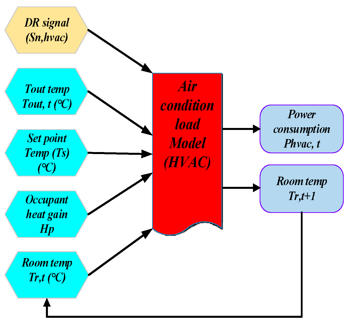
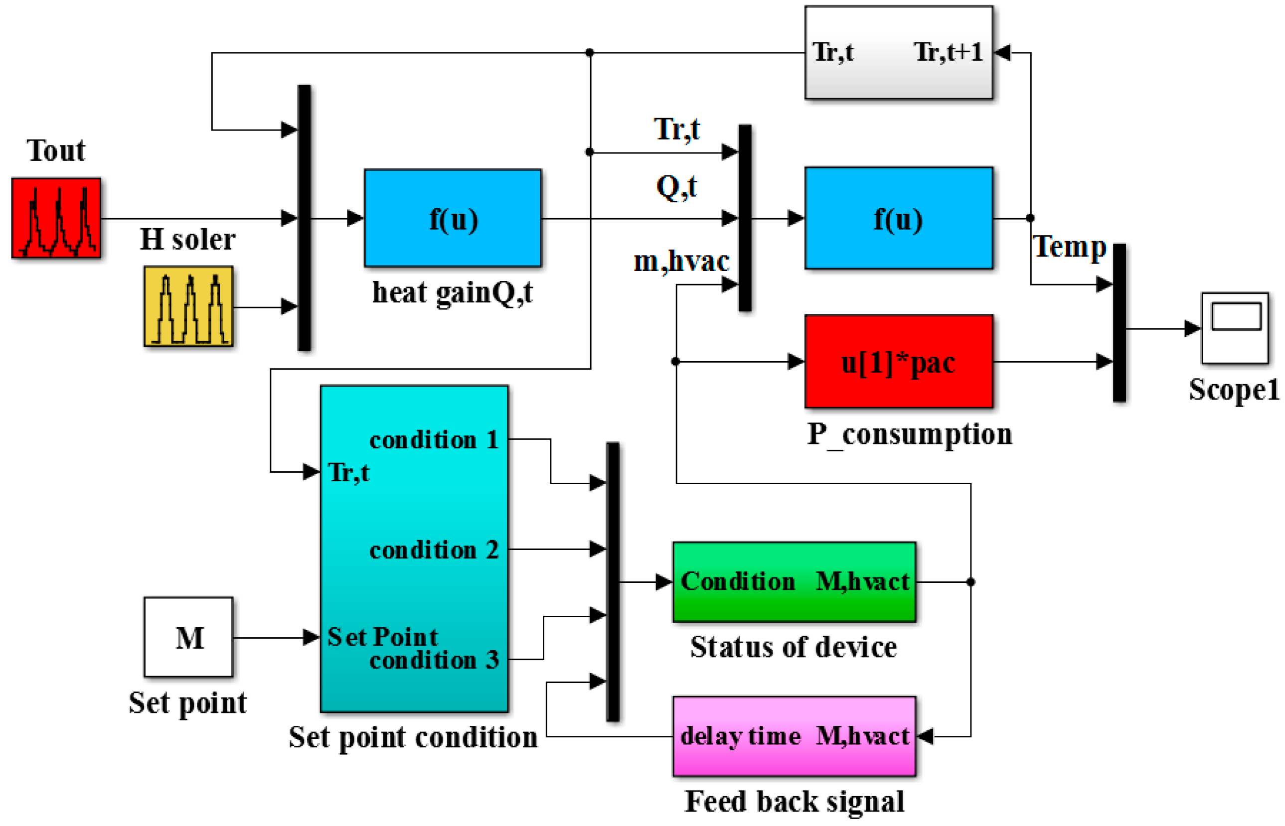
2.1. Air Conditioner Modeling

This section presents the AC load model development to produce a load profile at the distribution circuit level. To calculate the parameters that can be used with a physical-based AC model, the mathematical expressions should be derived to obtain an accurate AC load model. The mathematical model is presented as a set of equations to obtain the relationship between the output and input parameters, as shown in Figure 2.
The AC unit parameters can be divided into three categories, namely, the characteristics of AC, the set points of temperatures, and the building structures. The input parameters of the AC model are the occupant heat gain H p , room temperature at time t, T r , t , outside temperature   T out , t , set point temperature T s , t , and the signal of DR S n ewh , t . The model outputs are the room temperature, which is used as an input to the model at the subsequent step of time and energy consumption. Other parameters, such as the number of people in the home, room size, solar radiation, season, number of windows, house area, heat gain rate of the house, and cooling load capacity, should be considered in Simulink.
In the initial condition, the room temperature at time (t) should be determined based on the cooling load factor for glass/corrected cooling load temperature difference [24] as follows:
T r , t + 1 = T r , t   + d t ( m hvac , t C hvac d c + Q t d c )  
where Q t is the heat gain rate of the house, T r , t is the room temperature at time t ( ), d t is the length of time slot, d c is the energy that changes the air temperature in the Room 1   ( ), m hvac , t is the status of AC in the time slot, and C hvac is the cooling load capacity (Btu/ ) [25].
The output room temperature is used as an input room temperature to the AC model at the following time step. From Equation (1), the heat gain rate of the house, Q t , is expressed as:
Q t = S HGC + ( H p × N p ) + ( (   A fl R fl + A wal R wal + A ce R ce + A win R win + ( K × S × V hos   ) ) × ( T out , t T r , t   )   ) + A win s × H solar  
where H p is the occupant heat gain ( btu /h); N p is the number of people inside a room; K is the changes in room air in any time slot; ( A fl ,   A wall , A ce , A win ) are the areas of floor, wall, ceiling, and window of the dwelling in (m2), respectively; S HGC is the solar heat gain coefficient of a window [26]; (   R fl ,   R wal , R ce ,   A win )   are the average thermal resistance of the floor, wall, ceiling, and window in ( · m2 · h/ btu ), respectively; T out , t   is the outside temperature ( ) [27]; A win _ s is the window area facing south (m2);   S is the air heat factor ( btu / · m 3 ); and H solar is the solar radiation heat power (W/m2).
To change the room temperature by 1 °C to   btu / , the specific heat of air needs to be specified. The specific heat capacity of air, Cp, is 0.2099 / m 2 ·   , and the house volume, V hos , in m 3 , is included in Equation (3):
d c ( btu ) = C p   ( btu m 3 ) × V hos   ( m 3 )
The amount of AC power consumed in kW with a thermostat operating in OFF or ON mode and running at its rated power when switched on at a given interval, P havc , t , can be expressed as:
P hvac , t = m hvac   ×   P hvac
where m hvac is the status of the device; m hvac = 1 means that the device is turned on, and m hvac = 0 means that the device is turned off. P hvac is the AC rated power in kW.
The differences between the set point of AC and the lower or upper limit of the temperatures are called dead band. If the room temperature decreases below a set point minus the dead band temperature, then the AC unit is switched OFF. If the room temperature reaches its maximum set point plus the dead band temperature, then the AC unit is switched ON. However, if the room temperature is within its tolerable band, then the AC keeps the same status as described mathematically in Equation (5):
m hvac = [ 0 , T hvac , t < ( T s , t Δ T ) 1 , T hvac , t > ( T s , t + Δ T ) m hvac , t 1 , T s , t Δ T T hvac , t   T s , t + Δ T ]   ×   S n hvac , t  
The electric power demand of the AC load model depends on the DR signal, S n hvac , t . During a DR event, this signal, which originates from the revised thermostat set point, can be changed by end users. T s , t is the set point temperature, and Δ T is the dead band temperature (±2 °C).
By using Equations (1), (4) and (5), we simulate the component models of AC and the mathematical model in Matlab, as shown in Figure 3.

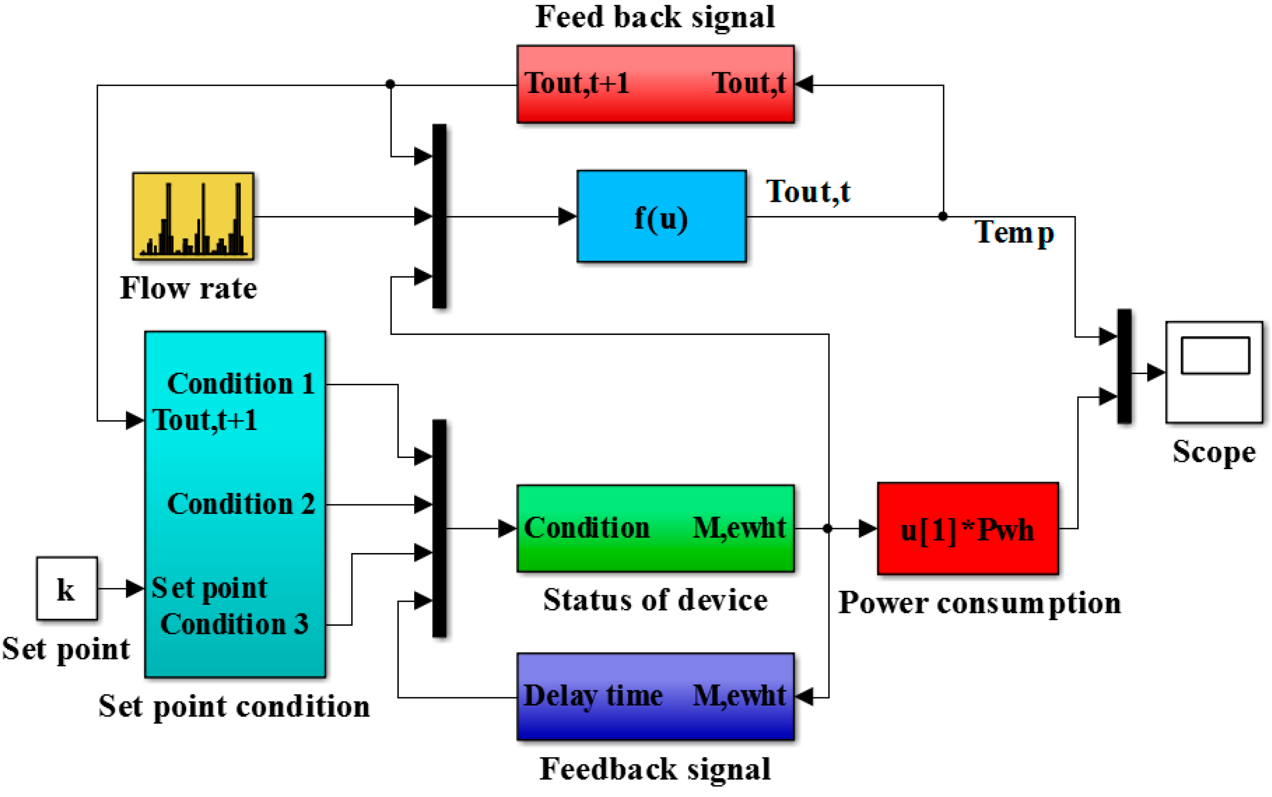
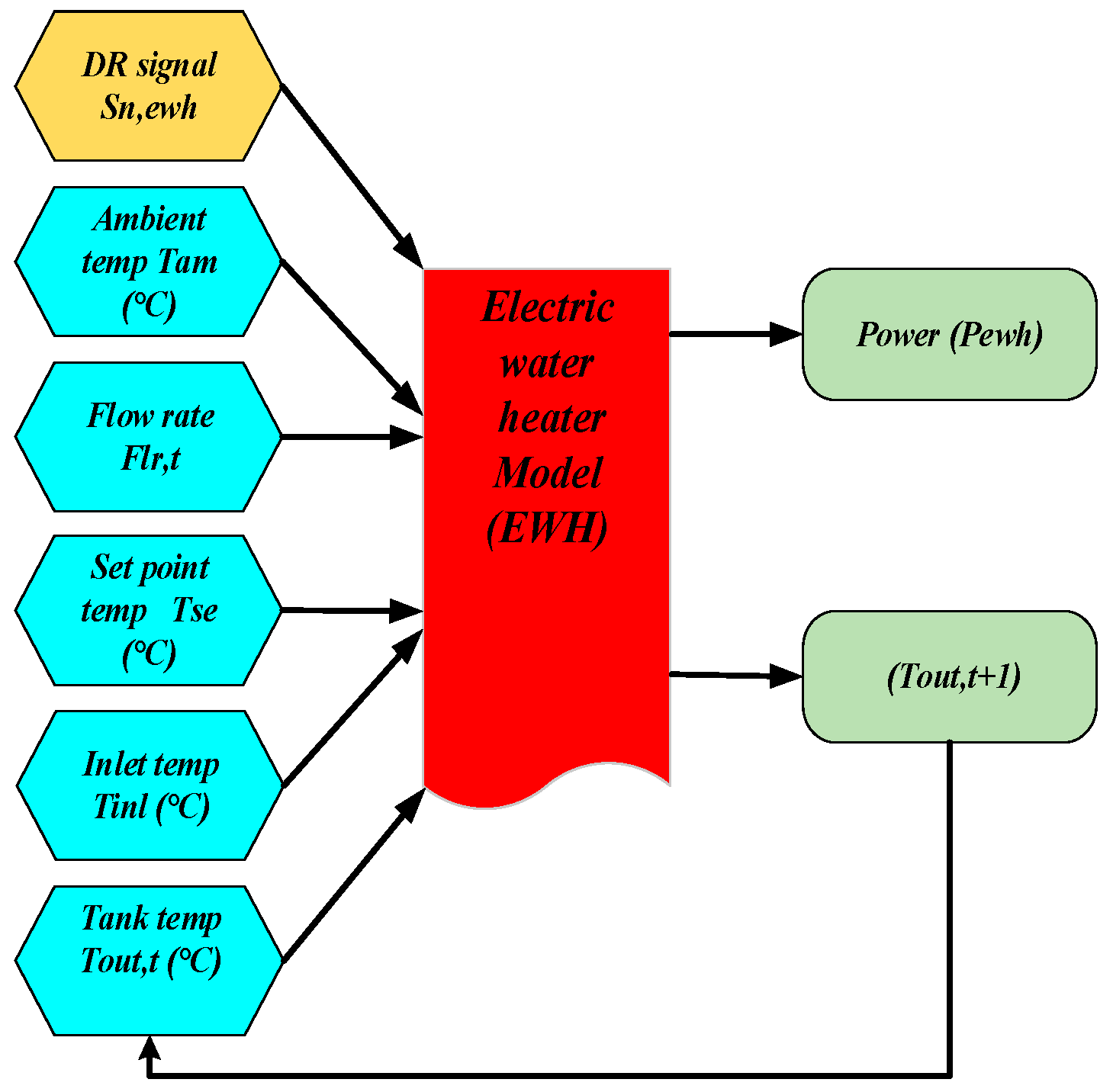
2.2. Electric Water Heater Modeling

The electric water heaters (EWHs) are among the major appliances that consume high energy in residential areas. Energy consumption depends on the amount of hot water that people use at home. To obtain an accurate model of EWH and to reflect any goal of DR strategies, EWH should be modeled for use in HEMSC by calculating the input and output parameters, as shown in Figure 4.
A domestic EWH consists of a thermostat to sense temperature and OFF/ON switch to heat water. The WH parameters can be divided into three categories, namely, the set point temperature, the use of hot water, and the device characteristics. The input parameters are the ambient temperature, T amp , water flow rate, F l r , t , temperature of inlet water ,   Tinl , the set point temperature, T se , t , temperature of water tank ,   T out , t , and signal of residential DR, S n ewh , t . The model output is the temperature of the EWH tank that is used as an input to the model at the subsequent step of time and power consumption.
The data for the EWH model depends on additional parameters, such as the surface area of storage tank WH, cross-sectional area, and volume that contribute to the design of accurate models.
In the initial condition, the water temperature at time (t) of the EWH should be calculated based on the usage pattern [25]. First, the outlet water temperature of the tank is considered, which is expressed as
T out , t + 1 =   (   T out , t × ( V o l tank V × d t ) + T inl × F l r , t × d t V o l tank   )   +   d t 60     × ( P ewh , t V o l tank   (   3412   BTU kwh   A tank × ( T out , t T amp ) R tank   )   )
where T inl is the inlet water temperature ( ), F l r , t is the hot water flow rate at a given interval (m3/s), V o l tank is the volume of the tank (m3), A tank is the surface area of the tank, T amp is the ambient temperature, R tank is the heat resistance of the tank ( · m3 · h/ btu ), and dt is the duration of the time slot t.
The differences between the set point lower and upper limits of the tank temperature are called dead band. If the water tank temperature drops below the set point lower limit minus the dead band temperature range, then the EWH coils are switched ON. If the water tank temperature is raised to its set point upper limit plus the dead band temperature, then the heating coils of EWH are switched OFF. The EWH operation depends on the device status, m ewh , which is mathematically expressed as:
  m ewh = [ 1 ,   T ewh , t < T se , t Δ T 0 , T ewh , t > T se , t + Δ T m ewh , t 1 , T se , t Δ T T ewh , t T se , t + Δ T ]   × S n ewh , t
where S n ewh , t is the DR signal, T se , t is the set point temperature, and Δ T is the dead band temperature (±2 ). The electric power demand of the EWH load model depends on the DR signal S n ewh , t .
The amount of EWH power consumed in kW depends on the thermostat that operates in the OFF/ON states and runs at its rated power [28]. The power of EWH at a given time is calculated by:
P ewh , t = m ewh   ×   P ewh  
where m ewh is the status of the device; and m ewh = 1 means that the device is switched on, and m ewh = 0 means that the device is switched off. P ewh is the EWH rated power in kW.
By using Equations (6)–(8), we simulate the component models of EWH and the mathematical model in Matlab, as shown in Figure 5.
During a DR event, the signal, which originates from the revised thermostat set point, can be changed by the homeowner. The data for the EWH model depend on the storage tank WH and other parameters that contribute to the design of the EWH physical model.

2.3. Water Heater and Refrigerator Modeling

WM is a home appliance operated by a motor connected to the agitator through a unit called transmission. WMs are divided into two categories depending on the positioning of their axis, namely, vertical axis WM and horizontal axis WM. The power consumption of WM at the residential sector accounts for approximately 7.2% of the total electricity consumption [29] and usually consists of an induction motor. In addition, the main electrical component of REF is the compressor, which is again an induction motor. Many different approaches are used to model the WM and REF. Real data are measured by using a power quality analyzer to obtain accurate WM and REF models. Matlab/Simulink is developed using resistors and reactance, as shown in Figure 6 and Figure 7, for WM and REF, respectively.
The rated power of WM depends on the stage of washing cycles, including washing, rinsing, and spinning, which last typically 55 min to finish the WM job at full load with 53 L of water.

3. Gathering Data for Household Appliance Models

Data were obtained in December 2015 by using a power quality analyzer to measure the power consumption of AC, WH, WM, and REF as shown in Figure 8 by considering a sample apartment house in the town of Kajang, Malaysia as a case study.
The input physical model of AC considered three important factors, namely, AC characteristics, temperature, and building characteristics. The temperature consisted of outdoor and indoor set points. The outside temperature was measured by a temperature and humidity sensor wireless data logger connected inside and outside residences, as shown in Figure 9.
Solar irradiation (H solar) was measured by using the Apogee Instruments pyranometer. The pyranometer is a silicon cell that is sensitive to a portion of the solar spectrum that estimates the total radiation across the entire solar spectrum, as shown in Figure 10. The REF data were obtained with a freezer temperature of −18 and refrigerator temperature of 3 , as shown in Figure 11. Thermal mass in the freezer and REF was combined and includes five bottles of water, two chickens, and 6 kg of fruits and vegetables in the REF at a working time of 24 h. The simulation model output result of REF after calculating the equivalent circuit of the motor depended on the measured data.
Each case of washing, rinsing and spinning has different power consumptions. By contrast, the REF power consumption depends on two cases: the first case has doors closed, and the second case denotes frequent opening of the doors. The temperature settings on the REF and freezer are 3 °C and −18 °C, respectively.
To simulate the model in Matlab, the equivalent circuit of MW and REF should be calculated to reflect the behavior of the real operation and to obtain an accurate result for both appliances. The equivalent circuit of the motor can be represented as impedances, as shown in Figure 12.

4. Artificial Intelligent Techniques Used for Home Energy Management Scheduling Controller

In this section, ANN, LSA, and the proposed hybrid LSA-ANN are discussed.

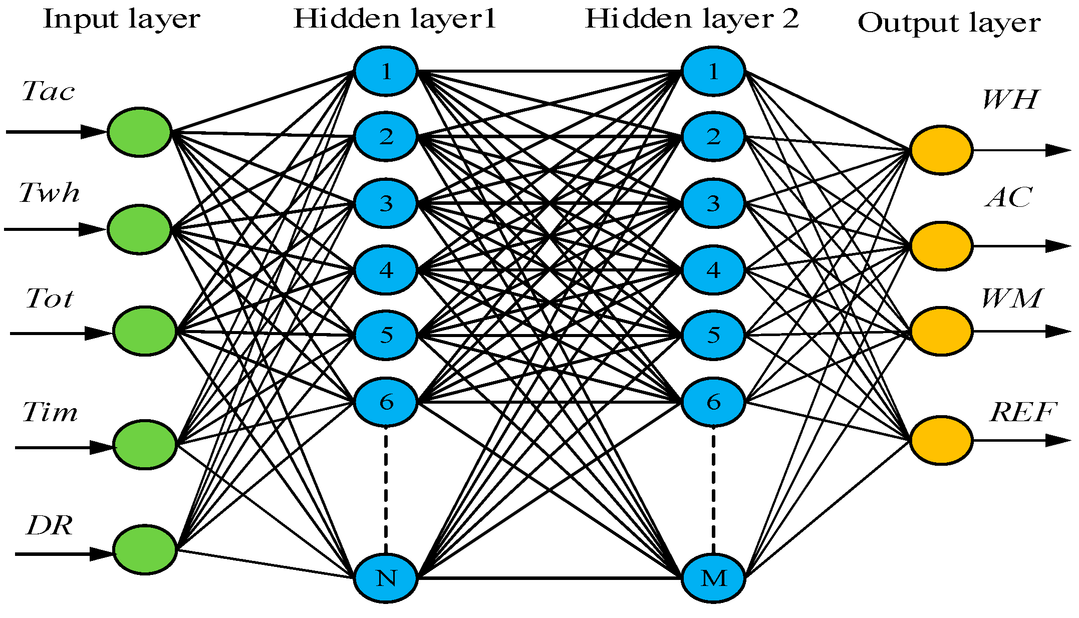
4.1. Artificial Neural Network Technique

An ANN is an information processing paradigm that models nonlinear systems and attempts to simulate the functionality of the human brain. Neural networks have many unique benefits, especially with the complex nonlinear relationships between system input and output, which handle any complex nonlinear functions through training and learning system input and output.
In this study, a feed-forward neural network type and the Levenberg–Marquardt training algorithm are selected for training the ANN in the Matlab toolbox. The ANN structure consists of five inputs ( T ac ,   T wh ,       T ot   ,       T im   ,     DR ), two hidden layers with the activation function as sigmoid function, and four outputs (AC, WH, WM, and REF). The actual data are collected from the simulation system, which represents the training data of the ANN, as shown in Figure 13.
All inputs and outputs of ANN-based HEMSC can be expressed by Equations (9) and (10):
Input =   [ T ac 1   T wh 1   T ot 1   T im 1   DL 1 T ac 2   T wh 2   T ot 2 T im 2   DL 2 : : T ac n     T wh n     T ot n T im n   DL n ]  
Output =   [ AC 1   WH 1   REF 1   WM 1 AC 2   WH 2   REF 2   WM 2 : :   AC n   WH n   REF n   WM n ]  
where T ac denotes the room temperature ( ); T wh is the WH temperature; T ot is the total power consumption; T im denotes the time of the system; and DR is the signal of a DR event.
In this system, the DR starts from between 16 h and 23 h, and the value of demand limit (DL) is assumed to be 3 kW. If T ot is higher than DL, then the controller will switch OFF the lower priority appliance; otherwise, the system works normally. The T ac and T wh of the system are used to evaluate the comfort level of the end users for AC and WH, respectively. The outputs of the ANN are the signals to turn the four home appliances ON or OFF according to customer preferences, comfort level, and priority of appliances. Sudden changes in the home appliances can be predicted by using ANN.

4.2. Overview of Lightning Search Algorithm

Optimization is a process to find the best solution to problems depending on the input variables after determining the objective function subjected to constraints. The objective function is often formulated based on a certain application and can take the form of minimal error, minimal cost, optimal design, and optimal management. LSA is a new optimization algorithm based on the natural phenomenon of lightning [29], and it is inspired by the probabilistic nature and sinuous characteristics of lightning discharges during a thunderstorm. LSA is organized from the mechanism of step leader propagation. This algorithm considers the participation of fast particles (projectiles) in the figuration of the binary tree structure of a step leader. Similar to other metaheuristic algorithms, LSA also needs a population to begin the search. The projectile suggests random solutions for corresponding problems to be solved by LSA. More details about LSA and basic ideas can be found in [30,31]. The step leaders are formed in the first phase because transition projectiles are ejected from the thunder cell in a random direction. Thus, the formula of uniform probability distribution is used for a random number of step leaders. The standard uniform distribution can be formulated as follows:
f ( x T ) = { 1 ( b a ) ,     for   a < x T b   0 , elsewhere }  
where x T is a random number that may provide a solution; and a and b are the lower and upper bounds of the solution space, respectively. The probability density function f ( x s ) of an exponential distribution [31] is shown by Equation (12):
f ( x s ) = { 1 μ e ( x s ( μ ) )   ,     for     x s b   0   ,     for     x s b   }  
After the initial is evaluated, the position and direction are updated with Equation (13):
p i NEW s = p i s   ± exprand   ( μ i )
where p i NEW s is the new projectile, and p i s is the old projectile.
The projectiles and the step leaders that have traveled close to the ground do not have adequate potential to ionize large sections in front of the leading edge. In this way, the lead projectile can be formulated as a random number taken from the standard normal distribution. The normal probability density function f ( x L ) is expressed as:
f ( x L ) = { 1 σ 2 π e (   x L μ ) 2   / 2 σ 2 }
where f ( x L ) is the normal probability density function, σ is the scale parameter, and μ is the shape parameter.
From Equation (14), the randomly generated lead projectile can search in all directions from the current position defined by the shape parameter. The scale parameter σ decreases exponentially to find the best solution. Therefore, the position of p L in step + 1 can be shown in Equation (15) [31]:
p NEW L = p L + normrand   ( μ L ,   σ L )
where p NEW L is the new lead projectile.

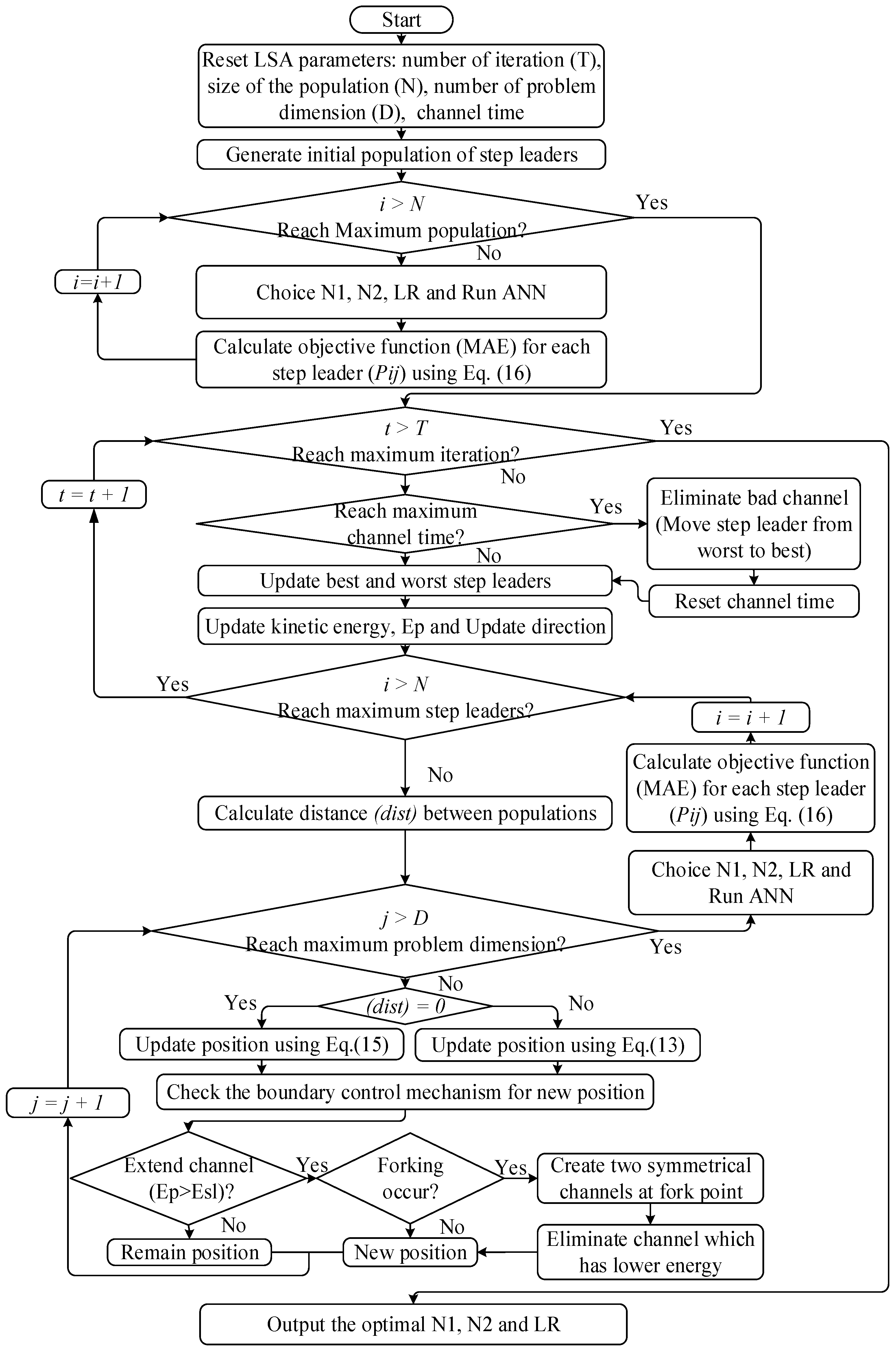
4.3. Proposed Hybrid Lightning Search Algorithm-Based Artificial Neural Network

The ANN algorithm can be used to control the appliances in HEMSC. The comfort level of end users can be utilized as the inputs of the ANN to determine and improve the suitable ON/OFF status of appliances and schedule another time without affecting the convenience of end users in the devices. The learning rate and the neurons in each hidden layer in the ANN architecture are the significant parameters. However, the selection of the learning rate and the neurons are subject to trial-and-error processes, which do not give the optimal solution. LSA addresses such a problem to enhance the ANN performance by finding the optimum learning rate and the best value of neurons in each hidden layer of the neural network that can be used in home energy scheduler controller. The implementation starts by resetting the LSA parameters, namely, number of iterations (T), population size (N), problem dimension (D), and channel time. Each step leader in this algorithm contains three components, namely, learning rate (LR), number of neurons in the first hidden layer (N1), and number of neurons in the second hidden layer (N2). The obtained values of LR, N1 and N2 are used in the ANN training to minimize the error of ON/OFF devices status in HEMSC. The flow chart of the proposed hybrid LSA-ANN is shown in Figure 14. The mean absolute error (MAE) is used as objective function to improve the performance of the ANN by minimizing the error function, as shown in the following equation:
M A E = i   =   1 n 1 n ( e r r o r ) 2
where e r r o r = s a s e , s a is the actual status, s e is the estimated status of HEMSC, and m is the number of samples.

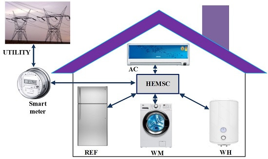
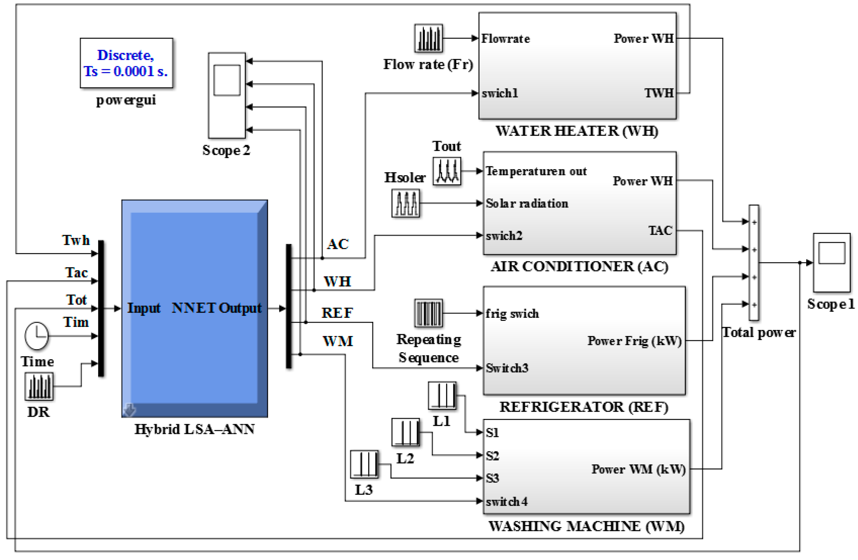
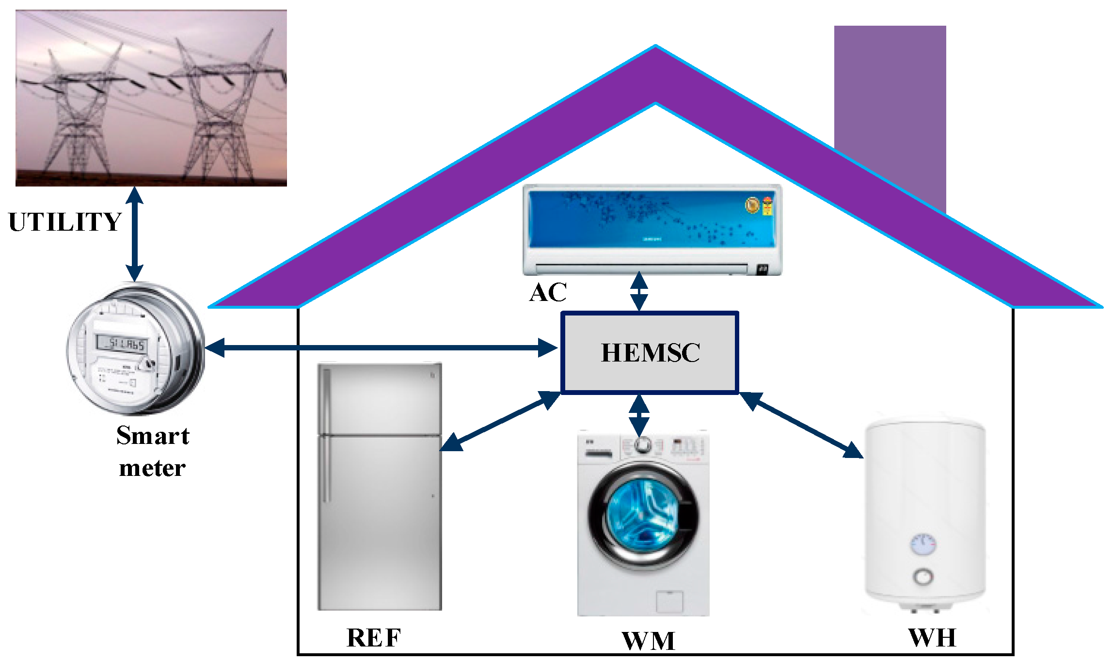
5. Overall Proposed Home Energy Management Scheduling Controller System

The proposed HEMSC algorithm is developed such that it can control and schedule the WH, AC, WM and REF, and switch customer load to decrease the costs of electrical power consumption during DR event. The HEMSC algorithm starts by reading the data and information of all the above-mentioned appliances. Each appliance is compared on several set points, including load priority, power consumption, and customer preference, by settings on the room temperature of AC and the water temperature of WH. The entire system is implemented by Matlab/Simulink, as shown in Figure 15.

6. Results and Discussion

This section describes the results of the simulation models of the home appliances with experimental results and the hybrid LSA-ANN results for the home energy management scheduling controller.

6.1. Home Appliance Simulation Result

The following subsections describe the simulation model results of the modeled home appliances.

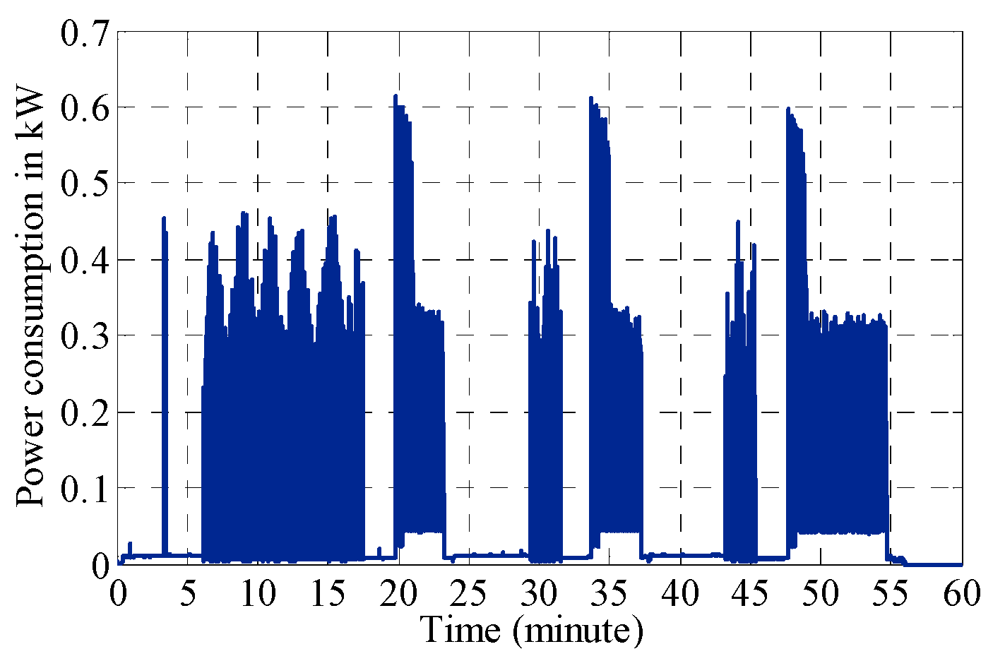
6.1.1. Water Heater Simulation Result

A case study is conducted to illustrate the performance model of the WH. This case study shows the hot water usage of WH at different times, as in Figure 16a. In Figure 16b, the maximum temperature is assumed to be 48 °C, and the minimum temperature of the WH setting is assumed to be 42 °C. These values can be altered in the physical model according to the preference of customers.
When the hot water is used at 7:00 a.m. and the temperature reaches its minimum allowable set point of 42 , the WH will switch ON to keep the water temperature at its comfortable range. When the hot water is used between 4:00 p.m. and 6:00 p.m., the WH will switch ON again to maintain the water temperature in the tank until the temperature reaches its maximum allowable set point of 48 , to switch OFF the WH. When the temperature of the water in the tank is within 42–48 , the heater switch status will maintain the previous device state.

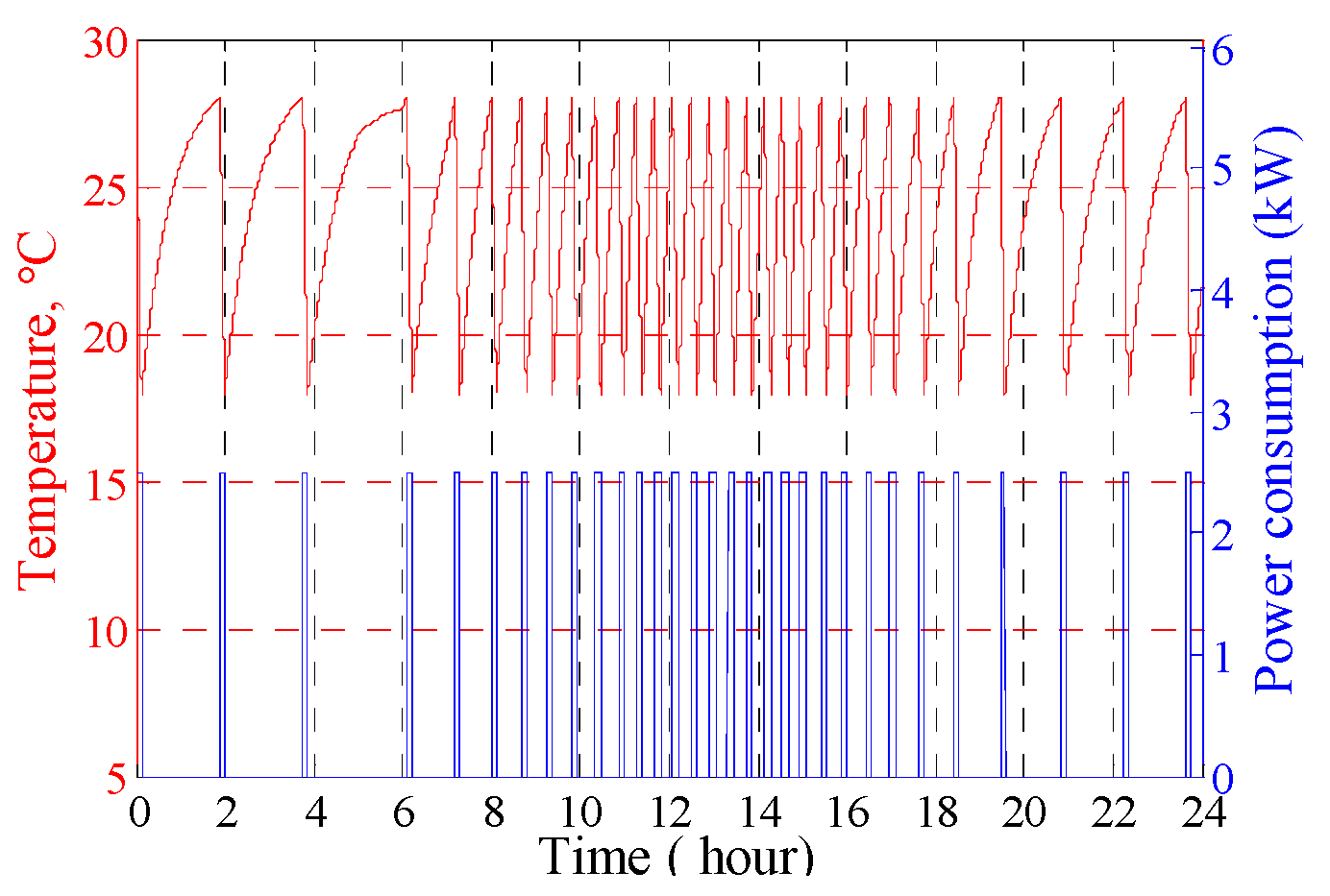
6.1.2. Air Conditioner Simulation Results

In the simulation, the maximum and minimum temperatures of AC are set at 28 °C and 18 , respectively. These values can be changed in the physical model according to the preference of the customer. Real data are measured to be used as input for the AC load model that includes the H solar and outside temperature, both of which are measured in Kajang, Malaysia. According to the homeowner comfort setting of the room temperature, which is set between 28 °C and 18 , the AC Simulink is shown in Figure 17.
Figure 17 shows that if the room temperature reaches its minimum set point temperature of 18 , then the AC is switched OFF. When the room temperature reaches its maximum set point temperature of 28 , then the AC is switched ON to keep the room temperature in its comfortable range. When the room temperature is within 18–28 , the switch status will maintain the previous device state.

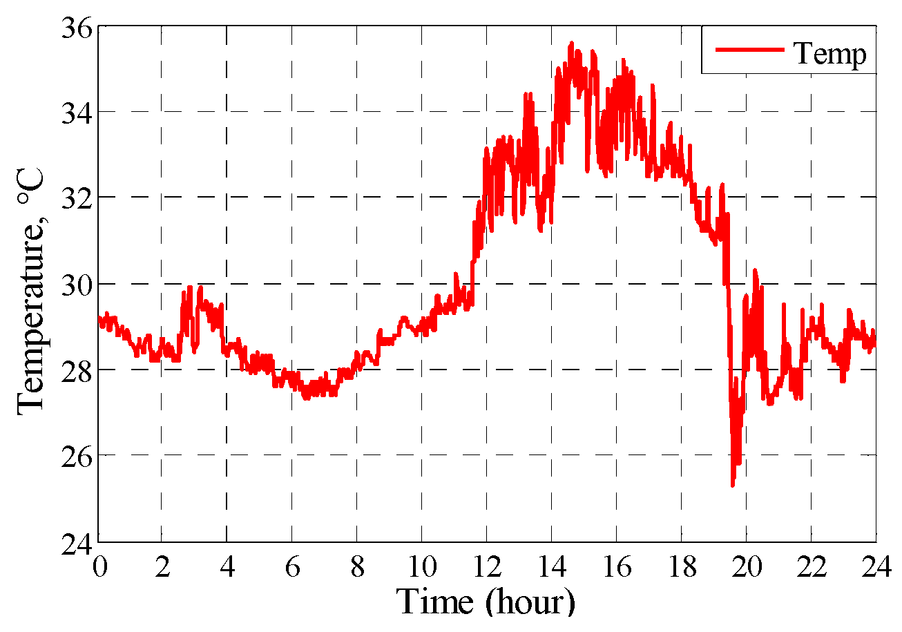
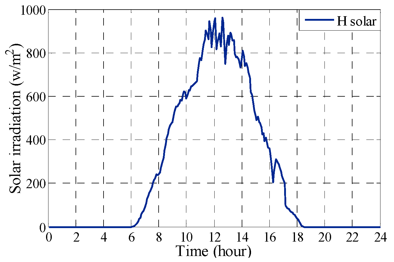
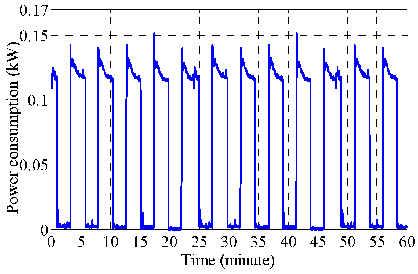
6.2. Experimental Measurement Data

The temperatures outside and inside the building were measured by using a wireless data logger sensor, and the measured outdoor temperature is shown in Figure 18. The solar irradiation was measured using the Apogee instrument pyranometer sensors and the measured data are shown in Figure 19. Both the temperature and solar irradiation were used as inputs to the AC model.
Other data from WM and REF power consumption were also considered. According to the real measurement of WM, 55.5 min was needed to complete the job with three different energy consumption levels during washing, rinsing, and spinning. In the washing cycle, three intervals at 11.5, 2.25 and 2.5 min were needed to finish the task. In the rinsing cycle, three duration times were needed to finish the job, with a 1 min interval. Finally, the last cycle needed 2.5, 2.5 and 6min to complete the job. The experimental measurement data of the WM power consumption are shown in Figure 20. The power consumption curve of the REF was measured every minute, as shown in Figure 21.

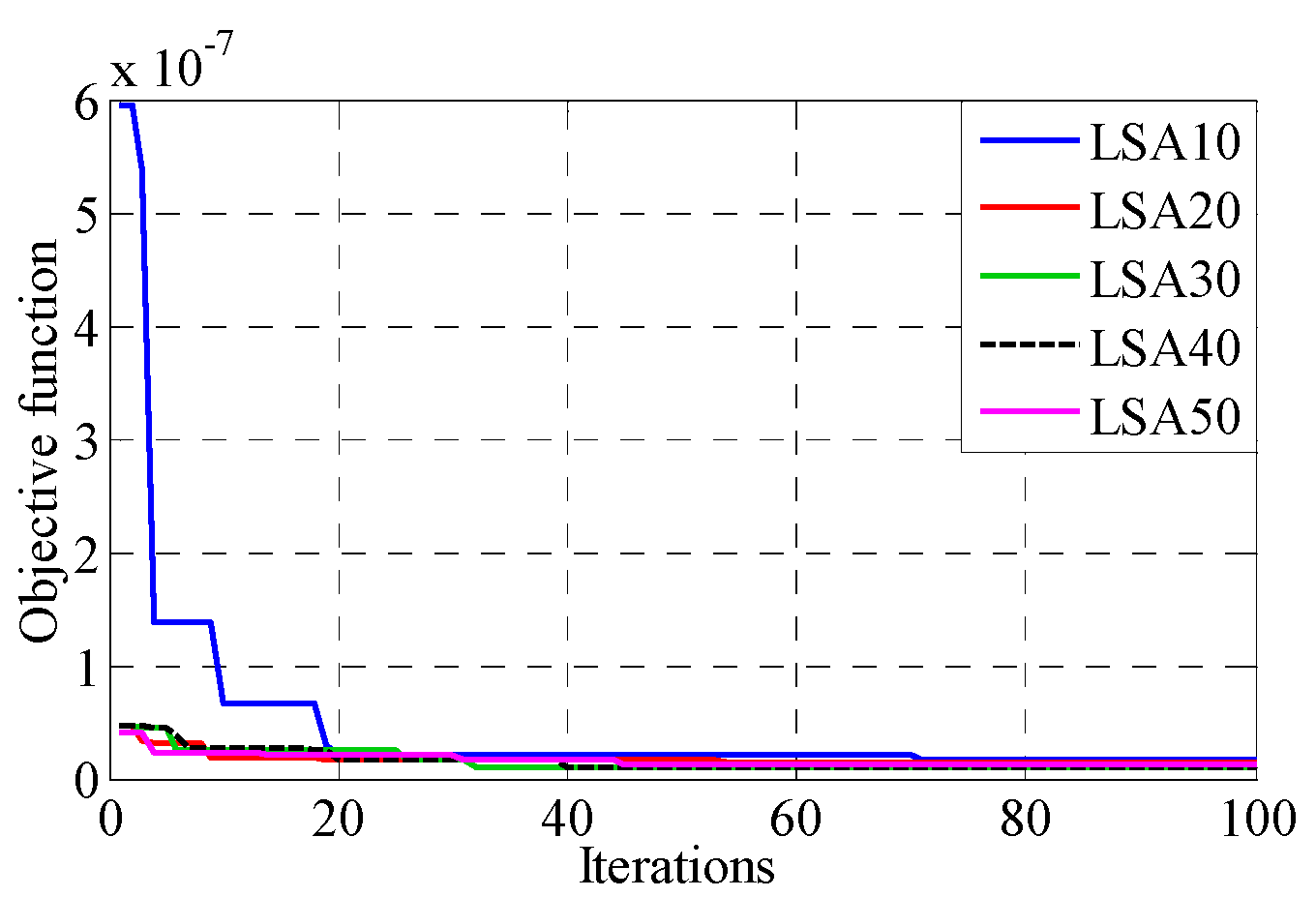
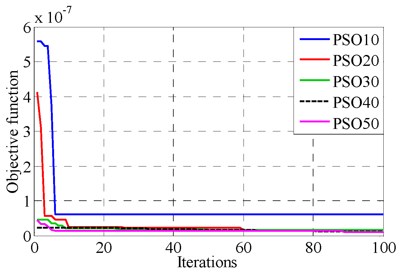
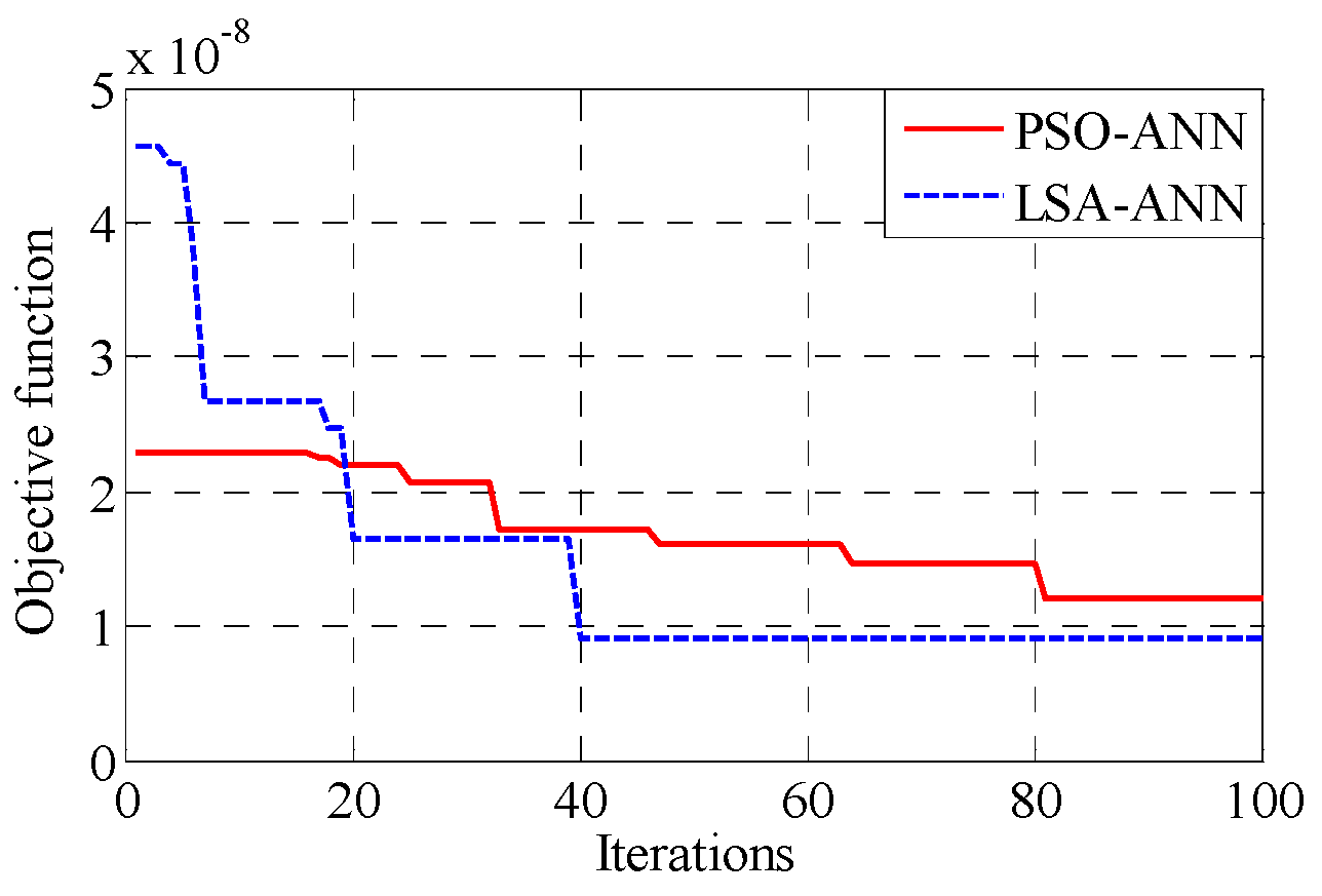
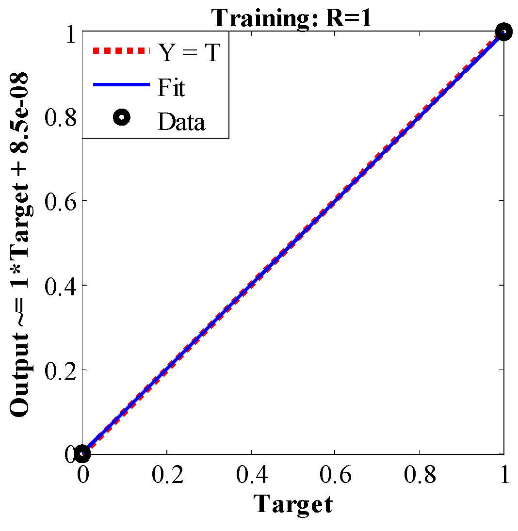
6.3. Results of the Hybrid Lightning Search Algorithm-Based Artificial Neural Network

The inputs of ANN include the room temperature T ac , WH temperature T wh , time of the system T im and total power consumption of the system   T ot . The signals are output to ON/OFF the WH, AC, WM, and REF. By using the ANN training and testing data, we can find all other parameters, such as inputs, number of neurons in each hidden layer, number of hidden layers, weights, learning rate, and output. LSA searches the best values for learning rate and the number of neurons in each hidden layer to enhance the ANN performance. The objective function for 10, 20, 30, 40 and 50 population sizes can be obtained, as shown in Figure 22. Several populations are executed to permit the LSA to select the population size to achieve the minimum error and the consumption time.
Figure 22 illustrates that the number of populations (N) as 40 can give the best result for the LSA than the population size numbers of 10, 20 and 30 because a high error and the objective function are achieved in error 9.128 × 10⁻⁹ after 40 iterations. The population size of 50 needs more working time than the population size of 40. The ANN parameters based on the results of the hybrid LSA-ANN are shown in Table 1. The PSO algorithm is also implemented to obtain the same objective for 10, 20, 30, 40 and 50 population sizes for comparison with the results from the hybrid LSA-ANN, as shown in Figure 23.
The obtained results from the hybrid LSA-ANN are compared with those from the hybrid PSO-ANN to validate the developed algorithm. The result of the hybrid LSA-ANN achieves a MAE error of 9.128 × 10⁻⁹ after 40 iterations at a population size of 40. The hybrid PSO-ANN obtains a MAE error of 1.195 × 10⁻⁸ after 81 iterations at a population size of 40, as illustrated in Figure 24.
The regression coefficient (R) close to unity and the value of R for training is 1. The performance of the hybrid LSA-ANN is shown in Figure 25.

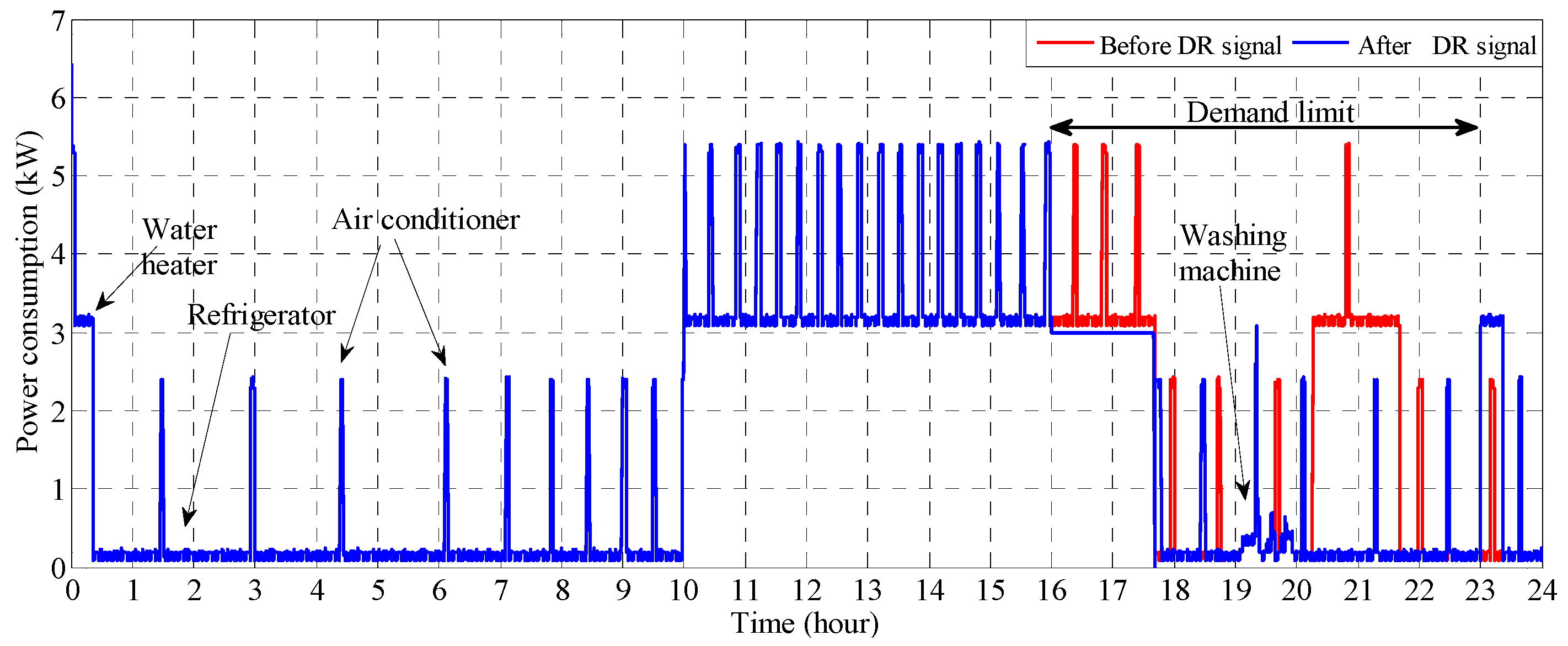
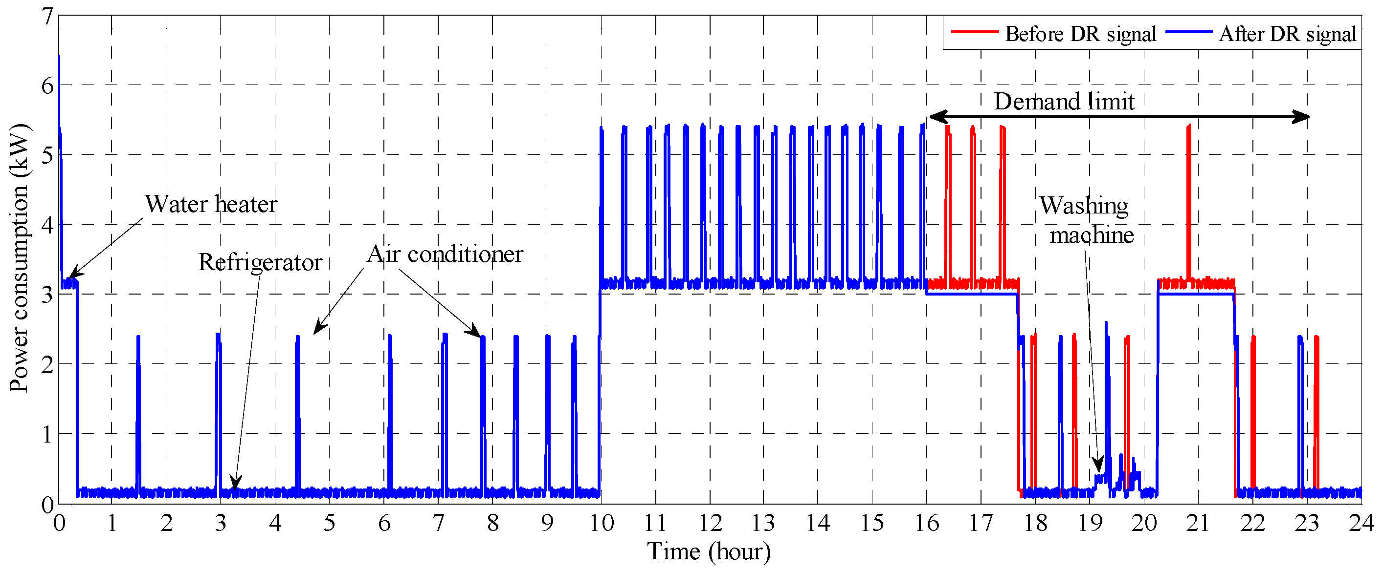
6.4. Results of the Proposed Hybrid LSA-ANN Based Home Energy Management Scheduling Controller

A DR event is usually imposed by the power utility to reduce the total power consumption at the peak period time with DL. The DR event is assumed to start from between 4:00 P.M. and 11:00 P.M., and DL is assumed to be 3 kW. If the total electrical power consumption is greater than the DL, then the HEMSC will turn OFF the appliance according to priority, starting with REF, and force the loads to shift and schedule their operating time after the DR event to keep the total power consumption below its DL. The HEMS issues a control signal to turn ON the appliance when the total household load is below its DL level. In this way, the HEMSC will optimize the scheduling of the appliances while maintaining the total power consumption below its DL.
Two case studies are considered to describe the implementation of the HEMSC algorithm. The first case does not apply the DR signal and the second case applies the DR signal by using the hybrid LSA-ANN, as shown in Figure 26. The second case using the hybrid PSO-ANN is shown in Figure 27 to clarify the performances of WH, AC, WM and REF, and to calculate the power saving.
Figure 26 and Figure 27 show that AC, WM, and REF have to be switched OFF, and one appliance, which is the WH, can be operated and draws 3 kW according to priority. The AC and REF require their schedules to be shifted to another period. The results explain the performance of the proposed HEMSC with the reduction of the total power consumption of the four home appliances at a specific time below the DL value. The algorithm prevents the total power consumption from exceeding the selected DL value. The energy saving for the total power consumption is 9.7138% per 7 h without any effect on the comfort level of the end users, whereas the energy saving for the total power by using the hybrid PSO-ANN is 2.3817% per 7 h. The power saving performance of the proposed hybrid LSA-ANN based HEMSC is better than that of the hybrid PSO-ANN.

7. Conclusions

This paper presents the application of LSA to solve the problems of ANN by finding the optimum learning rate and the best value of neurons in each hidden layer of the neural network that can be used in HEMSC. A comparison of results shows that the hybrid LSA-ANN used in HEMSC is better than the hybrid PSO-ANN in terms of scheduling household appliances and reducing the peak load while guaranteeing end user comfort associated with the operation of loads. The ANN ON/OFF estimation status is enhanced by minimizing the MAE. The hybrid LSA-ANN achieves a MAE error of 9.128 × 10⁻⁹, whereas the hybrid PSO-ANN achieves a MAE error of 1.195 × 10⁻⁸. The proposed algorithm shows a better response in switching the status in HEMSC. Therefore, the energy saving for the total power by using the hybrid LSA-ANN is 9.7138% per 7 h, whereas that by using the hybrid PSO-ANN is 2.3817% per 7 h. The results explain the capability of the proposed HEMSC algorithm to maintain the total electrical energy consumption below the DL value during a DR event. Moreover, the algorithm easily deals with the DR signals and is more effective in energy saving.

Acknowledgments

The authors gratefully acknowledge the University Kebangsaan Malaysia for the financial support for the project under research Grant No. DIP-2014-028.

Author Contributions

Maytham S. Ahmed is a Ph.D. student implementing the project and he is the corresponding author of the manuscript. Azah Mohamed is the main supervisor of the student who leads the project and edits the manuscript. Hussain Shareef is the co-supervisor of the student who has edited the manuscript and given valuable suggestions to improve the manuscript. Raad Z. Homod is the co-supervisor of the student who has edited the manuscript.

Conflicts of Interest

The authors declare no conflict of interest.

References

  1. Deploying a Smarter Grid through Cable Solutions and Services, 2010. Available online: http://www.nexans.com/Corporate/2010/WHITE_PAPER_SMART_GRIDS_2010.pdf (accessed on 9 August 2016).
  2. Hammond, G.P.; Pearson, P.J. Challenges of the transition to a low carbon, more electric future: From here to 2050. Energy Policy 2013, 52, 1–9. [Google Scholar] [CrossRef] [Green Version]
  3. Barton, J.; Huang, S.; Infield, D.; Leach, M.; Ogunkunle, D.; Torriti, J.; Thomson, M. The evolution of electricity demand and the role for demand side participation, in buildings and transport. Energy Policy 2013, 52, 85–102. [Google Scholar] [CrossRef] [Green Version]
  4. Huaman, R.N.E.; Tian, X.J. Energy related CO2 emissions and the progress on ccs projects: A review. Renew. Sustain. Energy Rev. 2014, 31, 368–385. [Google Scholar] [CrossRef]
  5. Yun, G.Y.; Kim, H.; Kim, J.T. Effects of occupancy and lighting use patterns on lighting energy consumption. Energy Build. 2012, 46, 152–158. [Google Scholar] [CrossRef]
  6. Richardson, I.; Thomson, M.; Infield, D.; Clifford, C. Domestic electricity use: A high-resolution energy demand model. Energy Build. 2010, 42, 1878–1887. [Google Scholar] [CrossRef] [Green Version]
  7. Horst, G.R.; Zhang, J.; Syvokozov, A.D. Total home Energy Management System. U.S. Patent 7561977 B2, 14 July 2009. [Google Scholar]
  8. Arif, M.T.; Oo, A.M.T.; Stojcevski, A. An investigation for improved home energy management. In Proceedings of the 2014 Australasian Universities Power Engineering Conference (AUPEC), Perth, Australia, 28 September–1 October 2014.
  9. Vardakas, J.S.; Zorba, N.; Verikoukis, C.V. A survey on demand response programs in smart grids: Pricing methods and optimization algorithms. IEEE Commun. Surv. Tutor. 2015, 17, 152–178. [Google Scholar] [CrossRef]
  10. Patel, K.; Khosla, A. Home energy management systems in future smart grid networks: A systematic review. In Proceedings of the 2015 1st International Conference on Next Generation Computing Technologies (NGCT), Dehradun, India, 4–5 September 2015; pp. 479–483.
  11. Farzamkia, S.; Ranjbar, H.; Hatami, A.; Iman-Eini, H. A novel PSO (particle swarm optimization)-based approach for optimal schedule of refrigerators using experimental models. Energy 2016, 107, 707–715. [Google Scholar] [CrossRef]
  12. Abd Ali, J.; Hannan, M.A.; Mohamed, A. A novel quantum-behaved lightning search algorithm approach to improve the fuzzy logic speed controller for an induction motor drive. Energies 2015, 8, 13112–13136. [Google Scholar] [CrossRef]
  13. Ali, J.A.; Hannan, M.; Mohamed, A.; Abdolrasol, M.G. Fuzzy logic speed controller optimization approach for induction motor drive using backtracking search algorithm. Measurement 2016, 78, 49–62. [Google Scholar] [CrossRef]
  14. Ibrahim, A.A.; Mohamed, A.; Shareef, H. Optimal power quality monitor placement in power systems using an adaptive quantum-inspired binary gravitational search algorithm. Int. J. Electr. Power Energy Syst. 2014, 57, 404–413. [Google Scholar] [CrossRef]
  15. Kang, S.J.; Park, J.; Oh, K.-Y.; Noh, J.G.; Park, H. Scheduling-based real time energy flow control strategy for building energy management system. Energy Build. 2014, 75, 239–248. [Google Scholar] [CrossRef]
  16. Mohsenian-Rad, A.H.; Leon-Garcia, A. Optimal residential load control with price prediction in real-time electricity pricing environments. IEEE Trans. Smart Grid 2010, 1, 120–133. [Google Scholar] [CrossRef]
  17. Haider, H.T.; See, O.H.; Elmenreich, W. Dynamic residential load scheduling based on adaptive consumption level pricing scheme. Electr. Power Syst. Res. 2016, 133, 27–35. [Google Scholar] [CrossRef]
  18. Hernandez, C.A.; Romero, R.; Giral, D. Optimization of the use of residential lighting with neural network. In Proceedings of the 2010 International Conference on Computational Intelligence and Software Engineering (CiSE), Wuhan, China, 10–12 December 2010.
  19. Pedrasa, M.A.; Spooner, E.D.; MacGill, I.F. Robust scheduling of residential distributed energy resources using a novel energy service decision-support tool. In Proceedings of the 2011 IEEE PES Innovative Smart Grid Technologies (ISGT), Anaheim, CA, USA, 17–19 January 2011.
  20. Setlhaolo, D.; Xia, X.; Zhang, J. Optimal scheduling of household appliances for demand response. Electr. Power Syst. Res. 2014, 116, 24–28. [Google Scholar] [CrossRef]
  21. Wang, Z.; Yang, R.; Wang, L. Multi-agent control system with intelligent optimization for smart and energy-efficient buildings. In Proceedings of the IECON 2010—36th Annual Conference on IEEE Industrial Electronics Society, Glendale, AZ, USA, 7–10 November 2010; pp. 1144–1149.
  22. Yuce, B.; Rezgui, Y.; Mourshed, M. ANN–GA smart appliance scheduling for optimised energy management in the domestic sector. Energy Build. 2016, 111, 311–325. [Google Scholar] [CrossRef]
  23. Gharghan, S.K.; Nordin, R.; Ismail, M.; Ali, J.A. Accurate wireless sensor localization technique based on hybrid PSO–ANN algorithm for indoor and outdoor track cycling. IEEE Sens. J. 2016, 16, 529–541. [Google Scholar] [CrossRef]
  24. Homod, R.Z.; Sahari, K.S.M.; Almurib, H.A.; Nagi, F.H. RLF and TS fuzzy model identification of indoor thermal comfort based on PMV/PPD. Build. Environ. 2012, 49, 141–153. [Google Scholar] [CrossRef]
  25. Shao, S.; Pipattanasomporn, M.; Rahman, S. Development of physical-based demand response-enabled residential load models. IEEE Trans. Power Syst. 2013, 28, 607–614. [Google Scholar] [CrossRef]
  26. U.S. Department of Energy. Building Energy Codes Progeam. Available online: http://www.Energycodes.Gov/support/shgc_faq.Stm (accessed on 15 May 2016).
  27. Kandar, M.; Nikpour, M.; Ghasemi, M.; Fallah, H. Study of the effectiveness of solar heat gain and day light factors on minimizing electricity use in high rise buildings. World Acad. Sci. Eng. Technol. 2011, 73, 73–77. [Google Scholar]
  28. Ahmed, M.S.; Shareef, H.; Mohamed, A.; Ali, J.A.; Mutlag, A.H. Rule base home energy management system considering residential demand response application. Appl. Mech. Mater. 2015, 785, 526–531. [Google Scholar] [CrossRef]
  29. Bertoldi, P.; Hirl, B.; Labanca, N. Energy Efficiency Status Report 2012; Joint Research Centre, European Commission: Ispra, Italy, 2012. [Google Scholar]
  30. Mutlag, A.H.; Mohamed, A.; Shareef, H. A nature-inspired optimization-based optimum fuzzy logic photovoltaic inverter controller utilizing an eZdsp F28335 board. Energies 2016, 9, 120. [Google Scholar] [CrossRef]
  31. Shareef, H.; Ibrahim, A.A.; Mutlag, A.H. Lightning search algorithm. Appl. Soft Comput. 2015, 36, 315–333. [Google Scholar] [CrossRef]
Figure 1. Block diagram of the proposed home energy management scheduling controller (HEMSC) system. AC: air conditioner; REF: refrigerator; WM: washing machine; WH: water heater.
Energies 09 00716 g001
Figure 2. Flowchart of the AC load model.
Energies 09 00716 g002
Figure 3. Matlab block for the simulation model of the AC load model.
Energies 09 00716 g003
Figure 4. Flowchart of the electric water heater (EWH) load model. DR: demand response.
Energies 09 00716 g004
Figure 5. Matlab block for the simulation model of the EWH load model.
Energies 09 00716 g005
Figure 6. Simulation model of WM.
Energies 09 00716 g006
Figure 7. Simulation model of REF.
Energies 09 00716 g007
Figure 8. Power quality analyzer to measure the power consumption.
Energies 09 00716 g008
Figure 9. Temperature and humidity wireless data logger.
Energies 09 00716 g009
Figure 10. Apogee Instruments pyranometer solar radiation sensors.
Energies 09 00716 g010
Figure 11. REF power consumption measurement.
Energies 09 00716 g011
Figure 12. Equivalent circuit of WM and REF.
Energies 09 00716 g012
Figure 13. Architecture of the artificial neural network (ANN) algorithm.
Energies 09 00716 g013
Figure 14. Flowchart of the proposed hybrid LSA-ANN.
Energies 09 00716 g014
Figure 15. Matlab block implementation for the simulation model of the overall system.
Energies 09 00716 g015
Figure 16. Simulation model of EWH load: (a) flow rate of the hot water in gpm; and (b) hot water temperature within 42–48 °C with the power consumption pattern.
Energies 09 00716 g016
Figure 17. Simulation model of AC power consumption pattern with room temperature.
Energies 09 00716 g017
Figure 18. Measured outdoor temperature.
Energies 09 00716 g018
Figure 19. Measured solar irradiation data.
Energies 09 00716 g019
Figure 20. Actual power consumption curve of WM load.
Energies 09 00716 g020
Figure 21. Actual power consumption curve of REF load.
Energies 09 00716 g021
Figure 22. Objective function with iteration of the hybrid LSA-ANN for different population sizes.
Energies 09 00716 g022
Figure 23. Objective function with iteration of the hybrid particle swarm optimization (PSO)-ANN for different population sizes.
Energies 09 00716 g023
Figure 24. Performance comparison of LSA and PSO.
Energies 09 00716 g024
Figure 25. Performance of the hybrid LSA-ANN.
Energies 09 00716 g025
Figure 26. Total power consumption before and after DR signal with the hybrid LSA-ANN.
Energies 09 00716 g026
Figure 27. Total power consumption before and after DR signal with the hybrid PSO-ANN.
Energies 09 00716 g027
Table 1. ANN-designed parameters.
ParameterValueType
Number of inputs5ANN inputs
Number of outputs4ANN outputs
Number of hidden layers2ANN hidden layer
Number of neurons in hidden layer N16Obtained from LSA
Number of neurons in hidden layer N24Obtained from LSA
Number of iterations1000ANN iterations
Learning rate0.6175Obtained from LSA

