An Application of Non-Linear Autoregressive Neural Networks to Predict Energy Consumption in Public Buildings

Abstract

This paper addresses the problem of energy consumption prediction using neural networks over a set of public buildings. Since energy consumption in the public sector comprises a substantial share of overall consumption, the prediction of such consumption represents a decisive issue in the achievement of energy savings. In our experiments, we use the data provided by an energy consumption monitoring system in a compound of faculties and research centers at the University of Granada, and provide a methodology to predict future energy consumption using nonlinear autoregressive (NAR) and the nonlinear autoregressive neural network with exogenous inputs (NARX), respectively. Results reveal that NAR and NARX neural networks are both suitable for performing energy consumption prediction, but also that exogenous data may help to improve the accuracy of predictions.

1. Introduction

According to the International Energy Agency, the building sector is the largest energy-consuming sector, accounting for one-third of total global energy consumption, as well as an equally important source of CO₂ emissions [1]. Around 90% of building emissions are produced to operate the HVAC—heat, ventilation, and air-conditioning—and lighting systems [2]. Thus, energy efficiency currently represents a highly relevant and important issue.

During the last few years, the development of new sensing technologies has led to the successful installation of monitoring devices in different environments and, consequently, the wide availability of real-time data being acquired from rather varied elements. However, due to the heterogeneity and diversity of these information flows, coming from very different sensors and sources, appropriate management is difficult. Buildings with energy management systems have much lower operating costs than those without. Therefore, forecasting models for energy consumption represent an essential factor for controlling energy costs and reducing environmental impact. The first target of the models is knowledge extraction, which means the extraction of behavioural patterns and detection of anomalies. Accordingly, specific applications for building efficient energy management systems have been recently explored, such as prediction of the energy demand and detection of consumption profiles [3].

There is plenty of research literature related to time series prediction. Therefore, there are a multitude of models and methodologies related to this field, applied to energy efficiency. Nagy et al. [4] suggest a generalized additive tree ensemble approach to predict solar and wind power generation. Yuan et al. [5] use autoregressive moving average model (ARIMA), grey model GM(1,1), and a hybrid model to forecast China’s primary energy consumption. Fumo and RafeBiswas [6] apply linear regression analysis to predict energy consumption in single-family homes. Mordjaoui et al. present a short-term electric load forecasting model using an adaptive neuro-fuzzy inference system [7]. Guo et al. [8] write about energy consumption prediction of heat pump water heaters based on grey system. Zhang et al. [9] apply support vector regression (SVR) to building energy consumption.

Due to the excellent results and noteworthy success achieved in real applications [10,11,12,13,14,15], artificial neural networks (ANNs) are held up as one of the most popular models. Several studies have illustrated that ANNs have produced better results when compared to other techniques [16,17,18,19]. One of the great advantages of ANNs is their potential to model non-linear data relationships. Furthermore, once trained, ANNs provide swift performance of the network. Karatasou et al. [20] employed neural networks to estimate energy consumption. Deb et al. [21] present a methodology to forecast diurnal cooling load energy consumption for institutional buildings. Gonzalez and Zamorreño [22] predict short-term electricity by means of feedback ANN. Likewise, Camara et al. [23] apply feedforward networks to forecast energy consumption in the United States.

In the real world, there are a huge amount of non-linear systems, or those whose behaviour is dynamic and depends on their current state. The dynamic recurrent neural network (RNN), the nonlinear autoregressive (NAR), and the nonlinear autoregressive neural network with exogenous inputs (NARX) are neural network structures that can be useful in these cases [24,25]. The first advantage of these networks is that they can accept dynamic inputs represented by time series sets. Time series forecasting using neural network (NN) is a non-parametric method, which means that knowledge of the process that generates the time series is not indispensable. On one hand, the NAR model uses the past values of the time series to predict future values. On the other hand, the RNN model does not need past time series values as inputs nor delays, since it has recurrent connections within its own structure.

In this study, we focus on an experiment using NAR and NARX neural networks to predict energy consumption in public buildings. Our goal is to provide a methodology framework to analyze the time series historical data of energy consumption, and to know if the mid-term prediction of such energy consumption can be achieved with these models. Moreover, we test both NAR and NARX models to study if the energy consumption depends solely on historical data, or if further external variables can be used to increase the accuracy of predictions. This study in public buildings (faculties and research centers) of the University of Granada (UGR) has been carried out as a test case. At this University, innovative management systems have been installed in the last few years; as a consequence we can obtain sufficient energy consumption data to carry out the experimentation. A minimum of the last two years of data will be used for each building analyzed.

The main goal of this study is to analyze different forecasting methods for energy consumption. To that end, we are also interested in the study of the impact of exogenous data on the forecasting. The results could be used to avoid unnecessary consumption: reducing costs in the long term, saving energy and decreasing the emission of harmful by products (the most dangerous of which is carbon monoxide) and providing an initial framework on which to build more complex decision-support systems.

The manuscript is organized as follows: Section 2 introduces the proposed methodology and the description of the artificial neural network methods. After that, Section 3 describes the phases of the methodology used in the study, comprising the processing of data, noise data management, transformations, and the process of training, test, and validation. Section 4 provides a description of the real data used, obtained from buildings at the University of Granada. Section 5 and Section 6 shows the experimentation with the proposed models and their results. Finally, Section 7 gathers the main conclusions obtained and makes proposals for future work.

2. Methodology

The current research was developed in three stages: firstly, the data collection and pre-processing; secondly, ANN modelling and, finally, the analysis of performance and comparison between two different network prediction models: NAR and NARX networks.

Previous work has shown that classic feedforward ANN may provide outstanding results in time series prediction tasks [7,10,11,12,13,14,24,25]. In this study, we have selected two neural network architectures aimed specifically at this problem to be used as prediction models for energy consumption. The first model is non-linear autoregressive neural networks (NAR), which are to forecast samples framed in a one-dimensional time series. We have also selected non-linear autoregressive networks with exogenous inputs (NARX), which expand multidimensional time series using external information to enhance time series prediction performance.

Each network model has its benefits and costs: NAR methods are simpler than NARX. Nevertheless, the latter model allows the use of additional information that may improve prediction accuracy. In a real situation, not every building has the same management system nor the same number of features: some only register consumption whilst others handle more information, such as external and internal temperature. The selected ANN models allow us to work with both approaches. The following subsections describe these models to solve the problem of energy consumption time series prediction.

2.1. NAR Model

In the majority of cases, time series applications are characterized by high variations and fleeting transient periods. This fact makes it difficult to model time series using a liner model, therefore a nonlinear approach should be suggested. A nonlinear autoregressive neural network [26,27], applied to time series forecasting, describes a discrete, non-linear, autoregressive model that can be written as follows [28]:

$$y(t)=h(y(t-1), y(t-2), \dots , y(t-p))+ϵ(t)$$

(1)

This formula describes how a NAR network is used to predict the value of a data series $y$ at time t, y(t), using the $p$ past values of the series. The function h(·) is unknown in advance, and the training of the neural network aims to approximate the function by means of the optimization of the network weights and neuron bias. Finally, the term є(t) stands for the error of the approximation of the series y at time t.

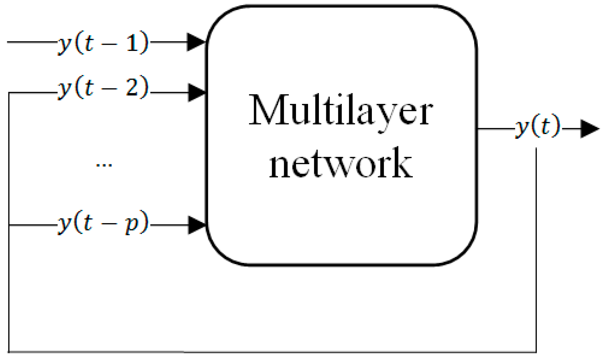
The topology of a NAR network is shown in Figure 1. The $p$ features y(t−1), y(t−2), …, y(t−p), are called feedback delays. The number of hidden layers and neurons per layer are completely flexible, and are optimized through a trial-and-error procedure to obtain the network topology that can provide the best performance. Nevertheless, it is important to bear in mind that increasing the number of neurons makes the system more complex, while a low number of neurons may restrict the generalization capabilities and computing power of the network.

The most common learning rule for the NAR network is the Levenberg-Marquardt backpropagation procedure (LMBP) [29,30,31,32]. This training function is often the fastest backpropagation-type algorithm. The LMBP algorithm was designed to approximate the second-order derivative with no need to compute the Hessian matrix, therefore increasing the training speed. When the performance function has the form of a sum of squares (frequently in feedforward network training), then the Hessian matrix can be approximated as shown in Equation (2) and the gradient can be computed as described in Equation (3).

$$\mathbf{H}={\mathbf{J}}^T\mathbf{J}$$

(2)

$$\mathbf{g}={\mathbf{J}}^T\mathbf{e}$$

(3)

In Equations (2) and (3), $\mathit{J}$ is the Jacobian matrix which contains the first derivatives of the network errors with respect to the weights and biases, and $\mathbf{e}$ is a vector of network errors in all training samples. To estimate the Jacobian matrix, the study in [32] uses a standard backpropagation algorithm to approximate the Hessian matrix. This approach is simpler than computing the Hessian matrix. The LMBP algorithm uses this approach in the Newton-like update described in Equation (4).

$${\mathbf{x}}_{k+1}={\mathbf{x}}_k-{[{\mathbf{J}}^T\mathbf{J}+\mu \mathbf{I}]}^{-1}{\mathbf{J}}^T\mathbf{e}$$

(4)

It should be noted that this method uses the Jacobian matrix for calculations, assuming that the performance function is the mean of the sum of the squared errors. Hence, networks must use either the mean square error (MSE) or error sum of squares (SSE), stated in Equations (5) and (6), where y_i stands for the i-th data sample, $\widehat{y_i}$ is the approximated data obtained by the network for the value y_i, and n the number of data samples for the network training.

$$SSE={\displaystyle \sum _{i=1}^n}{(\widehat{y_i}-y_i)}^2$$

(5)

$$MSE=\frac{SSE}{n}$$

(6)

In this study, we use NAR neural networks to model energy consumption time series as follows: the network structure contains one input (corresponding to the energy consumption at time t−1, y(t−1)), and one output (the next value of the time series, y(t), to be predicted). The number of delays is set experimentally after a data pre-processing and analysis stage.

2.2. NARX Model

In many real applications, there is an important correlation between the modelled time series and additional external data. In [4] it is indicated that a usual feature of renewable energy is that the output of power plants largely depends on weather conditions. Thus, the integration of knowledge or data about weather could benefit the time series modelling process to provide an accurate forecast instead of a unique approach with one single value corresponding to the consumption data [17,33].

The model nonlinear autoregressive with exogenous (External) inputs (NARX) is proposed in [34]. NARX predict series $y(t)$ given $p$ past values of series $y$ and another external series $x(t)$, which can be single or multidimensional. The equation that models the NARX network behaviour for time series prediction is shown in Equation (7).

$$y(t)=h(x(t-1), x(t-2), \dots , x(t-k), y(t-1), y(t-2), \dots , y(t-p))+ϵ(t)$$

(7)

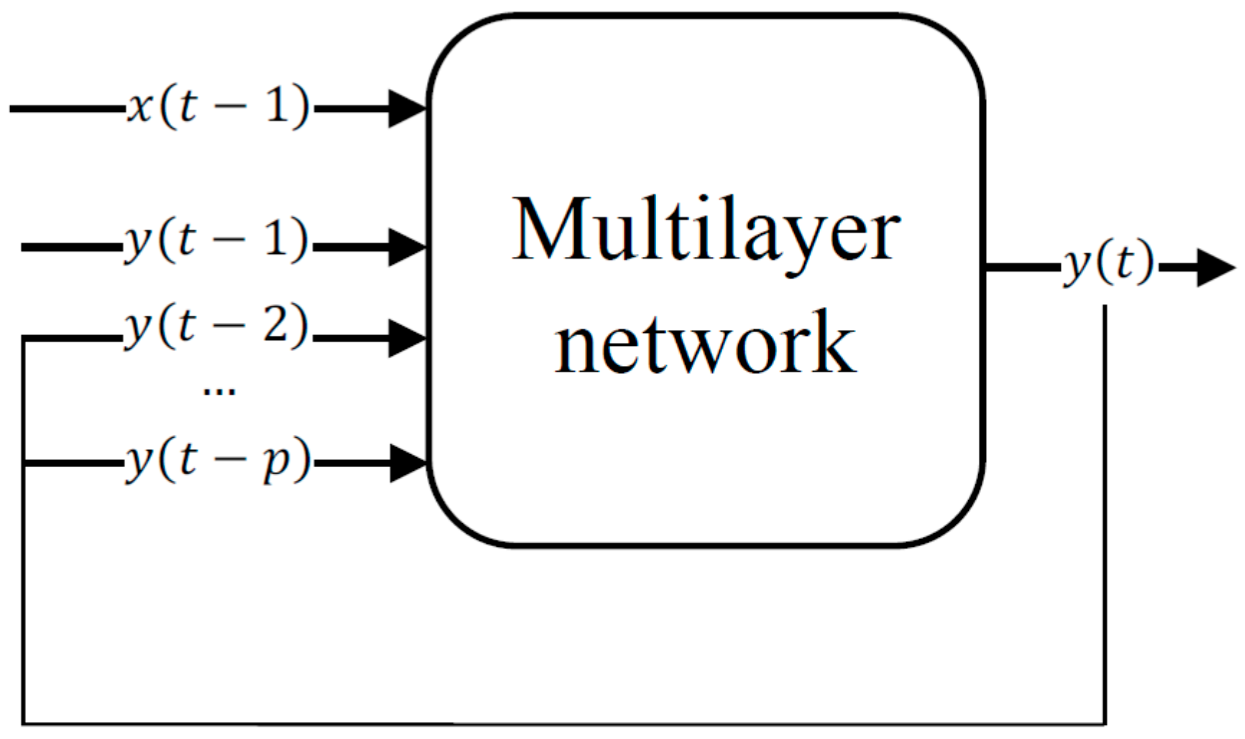
The NARX is a nonlinear model which estimates the future values of the time series based on its last outputs and external data. In this study, we use NARX with one input for the energy consumption time series at time t-1, y(t-1), and another input with exogenous data at time t−1, x(t−1), to provide a single output data y(t), corresponding to the value of the energy consumption one step forward. Figure 2 shows this architecture, similar to the NAR network. The only difference is in input; henceforth, output $y(t)$ takes account of the external data as it appears in the Equation (7). The learning rule LMBP, previously explained, is also used to train this model. Despite the flexibility of NARX to model exogenous input to help improve results by modelling external dependencies, NAR models are a good alternative because of their simplicity, as discussed in [35]. In the experimental section, we make a comparison of both approaches.

3. Energy Time Series Modelling and Forecasting

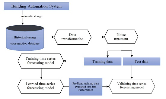
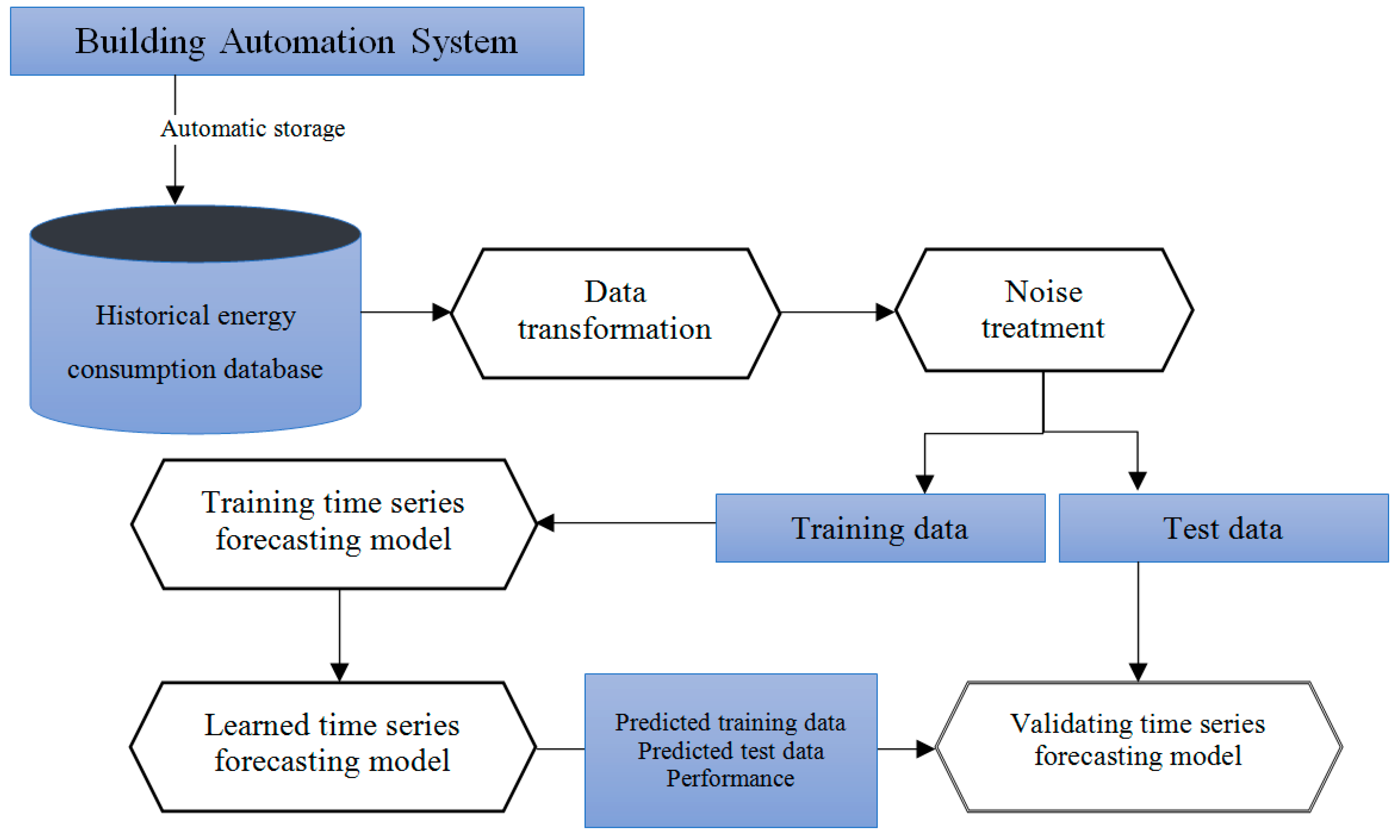
This section describes the process used to obtain an energy time series model, along with the forecasting methodology to predict the consumption in a building. The process overview is shown in Figure 3. There is no learning model indicated, so that it can support any of them without distinction. In other words, the methodology is general and can be utilized for both NAR and NARX neural networks. Each stage is detailed as follows:

(a)

Building automation system: software designed to support building energy management, which is made up of several components that provide coordinated control. It collects, summarizes and presents building data in usable way.

(b)

Historical energy consumption database: stores the building’s energy use (consumption, energy and power recorded and monitored by diverse sensors), as well as some external information such as temperature. In particular, we study the relationship between temperature and energy consumption using NARX models. The experimental section shows the results and conclusions obtained.

(c)

Data transformation: the building automation system is responsible for the storage of raw data. This information must be processed in order to change the consumption time scale and to extract the consumption data from the raw sensor storage. Regarding the time scale, some manuscripts propose a model for forecasting hourly [15,22,36]. However, most short-term forecasting problems involve predicting events for only a few time periods in a scale of days, weeks, or months [36]. Hence, our experimentation is focused in this context.

(d)

Noise treatment: the data captured from the physical world by sensor devices are sometimes incomplete, noisy and unreliable. This noise is mainly due to fault detection, a broken device or a connection failure. Two main strategies are pursued: (1) moving-average filter [37]—see Equation (8)—to remove outliers; and (2) linear interpolation, based on the values at neighbouring grid points to fill missing values.

$$y(n)=\frac{1}{windowsSize}·\left(x(n)+x(n-1)+\dots +x\left(n-(windosSize-1)\right)\right)$$

(8)

(e)

Train and test: the database is divided into 70% training data and 30% test data. The training and test data are selected randomly from the initial consumption dataset.

(f)

Training time series forecasting model: its aim is to fit the model using the training data. NAR and NARX models have been trained using LMBP as the training function and hyperbolic tangent sigmoid transfer function [38] for the neurons of intermediate layers. The parameters will be detailed in the experimental section. The models are trained with 70% of the days collected, and are tested with the remaining 30% of the data.

(g)

Learned time series forecasting model: once the model is trained, we test the prediction models to know their performance in training data sets and we store these results in a database.

(h)

Validating time series forecasting model: the final step is to verify that accurate results have been obtained, comparing the test data prediction with test data isolated in step 5. This dataset has not previously been used to train the network and can be used to know if the networks have correctly learned the time dependencies of the consumption data.

4. Data Collection Process

Smart management systems collect a multitude of information, monitored in real-time. In this paper, data are obtained from an actual building automation system (BAS). BAS is an automatic centralized control of the building’s heating, ventilation, air conditioning and lighting systems. This BAS is used by the University of Granada (UGR) (Granada, Spain) to monitor its buildings’ consumption, in order to analyze the information coming from several sources with the ultimate objective of better understanding of how and when energy is consumed in the distributed facilities. Data are generated and stored in a fine-grained fashion, which hinders the processes of data analysis and decision-making. The information should, therefore, be summarized and simplified in order to make useful forecasting.

The UGR has access to energy consumption and climatic data gathered in the buildings. In each campus, different kinds of buildings and sensor setups can be found. Teaching—units’ faculties, schools, and departments—is divided throughout five campuses—Centro, Cartuja, Fuentenueva, Aynadamar, and Ciencias de la Salud—which are distributed in different areas of the city of Granada. In addition, the UGR has centres in the autonomous cities of Ceuta and Melilla which are located in separate campus. Overall, the UGR is associated with 22 faculties, 5 schools, 8 training centres and five culture, sport, and service centres.

Each building consumption dataset is grouped by area. Therefore, it is assumed that there is a relationship between those buildings. Eight buildings belonging to the same compound have been selected for this energy consumption experimentation. Due to anonymity, the building consumptions are labelled as Building 1, Building 2, Building 3, and Building 8. These consumptions have been selected in the following way: the first and second buildings are chosen from the same compound, the third and fourth in the same way, etc. We have selected two representative buildings from four campuses to study the general energy consumption at the UGR.

4.1. Data Selection

Data selection was carried out by a preliminary pre-processing of all data coming from several faculties and determined buildings. After obtaining the data to be used to model the ANN, the subsequent step was to separate the data into two parts: training dataset and test dataset. All of the data were normalized to have the same range of values for each of the inputs to the ANN model. This guarantees that there are no attributes which are more important than others because of data ranges, and also eases a stable convergence of network weights and biases.

All data associated with energy consumption are stored hourly in the Historical Energy Consumption Database, and these data are the raw values obtained from energy counters. Thus, one sample of the raw consumption data describes the aggregate sum of all previous consumption until that moment. In this piece of research, data have been transformed in consumption registered per hour, so that one sample of the transformed data shows the consumption that took place precisely in that hour.

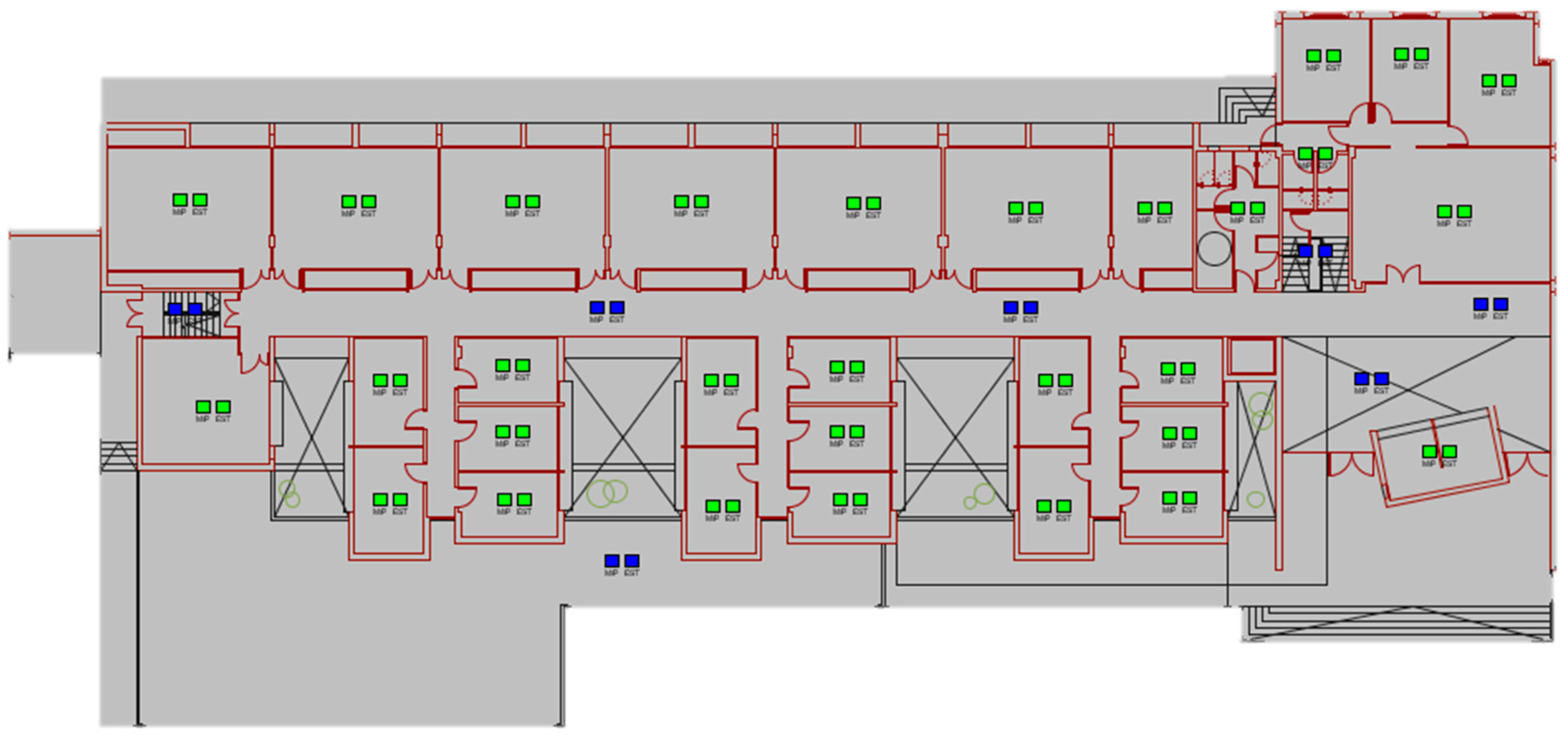
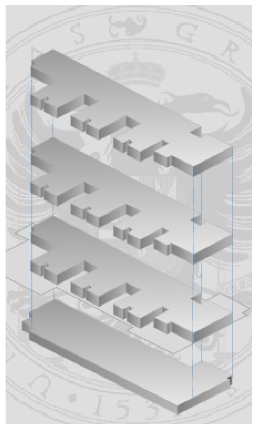
4.2. Sample Building

This subsection aims to summarize one sample building structure and to describe in detail the main characteristics and parameters monitored in the building compound. The selected building is comprised of four floors: basement, ground floor, first floor, and second floor (see Figure 4).

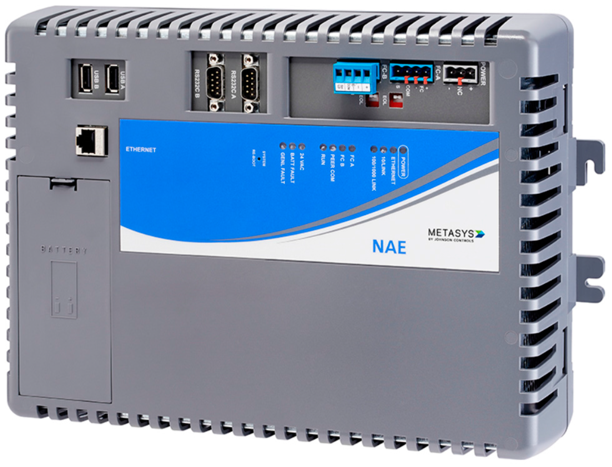
Each floor monitors three different types of information: lighting, electricity, heating and air conditioning. This building has a network automation engine—NAE—which delivers comprehensive equipment monitoring and control through features such as scheduling, alarm and event management, energy management, data exchange, data trending, and data storage. This tool helps lower efficiency costs for buildings. The MS-NAE5520-2 is the specific model used in this building (see Figure 5).

The MS-NAE5522-2 device supports a LonWorks trunk, two N2 Bus trunks or two BACnet MS/TP (RS-485), or a mixture of one N2 Bus trunk and one BACnet MS/TP trunk. It supports a maximum number of 255 devices on the LonWorks trunk and a maximum of 100 devices on each N2 Bus or BACnet MS/TP trunk. Its technical characteristics are summarized as follows:

• Power requirement: Dedicated nominal 24 VAC, Class 2 power supply (North America), SELV power supply (Europe), at 50/60 Hz (20 VAC minimum to 30 VAC maximum).
• Power consumption: 50 VA maximum.
• Ambient operating conditions: 0 to 50 °C (32 to 122 °F); 10% to 90% RH, 30 °C (86 °F) maximum dew point.
• Ambient storage conditions: −40 to 70 °C (−40 to 158 °F); 5% to 95% RH, 30 °C (86 °F) maximum dew point.
• Data protection battery: Supports data protection on power failure. Rechargeable gel cell battery: 12 V, 1.2 Ah, with a typical life of 3 to 5 years at 21 °C (70 °F); Product Code Number: MS-BAT1010-0.
• Clock battery: Maintains real-time clock through a power failure. Onboard cell; typical life 10 years at 21 °C (70 °F).
• Processor: 1.6 GHz Intel® Atom™ processor.
• Memory: 4 GB (2 GB partitioned) flash nonvolatile memory for operating system, configuration data, and operations data storage and backup, 1 GB SDRAM for operations data dynamic memory.
• Operating system: Johnson Controls OEM Version of Microsoft Windows Standard 2009.
• Network and serial interfaces: One Ethernet port; connects at 10 Mbps, 100 Mbps, or 1 Gbps; eight-pin RJ-45 connector. Two optically isolated RS-485 ports; 9.6 k, 19.2 k, 38.4 k, or 76.8 k baud; pluggable and keyed four-position terminal blocks (RS-485 ports available on NAE55 models only). Two RS-232-C serial ports, with standard nine-pin sub-D connectors, that support all standard baud rates. Two USB serial ports; standard USB connectors support an optional, user-supplied external modem. Options: One telephone port for internal modem; up to 56 kbps; six-pin modular connector. One LONWORKS port; FTT10 78 kbps; pluggable, keyed three-position terminal block (LONWORKS port available on NAE552x-x models only).
• Housing: Plastic housing with internal metal shield. Plastic material: ABS + polycarbonate UL94-5VB Protection: IP20 (IEC 60529).
• Mounting: On flat surface with screws on four mounting feet or on dual 35 mm DIN rail.
• Dimensions (Height × Width × Depth): 226 × 332 × 96.5 mm including mounting feet. Minimum space for mounting: 303 × 408 × 148 mm.

The energy management system in this building monitors different features, such as voltage, intensity, and power, which are collected in their different phases:

• Voltage phase R, S and T-neutral (V).
• Intensity phase R, S and T (A).
• Active power phase R, S and T (kW).
• Reactive power phase R, S and T (kVAR).
• Power factor phase R, S and T.
• Three-phase active power (kW).
• Frequency (Hz).
• Voltage phases: R-S, S-T and T-R (V).
• Energy consumed (kWh).
• Neutral intensity (A).
• Maximum demand (kW).
• Total harmonic distortion (%).

Furthermore, there are other devices used to monitor the lighting state. Figure 6 shows the state of a lamp in a room. A green state indicates that a light is on, and a blue state indicates that a light is off. Moreover, there is a pair of indicators for each room, the left one specifies the order—for example, if a light is going to power off in 30 seconds it appears in blue—and the right box shows the real state.

This figure shows how all the lamps are on in all the rooms, except in the corridor and the stairs.

All of these counters are gathering information 24 h a day, every day of the year. However, not all data are stored permanently; some features, such as lamp states or the state of a valve, are not saved in the long term. This research is concentrated mainly on the energy consumption registered and the temperature measured.

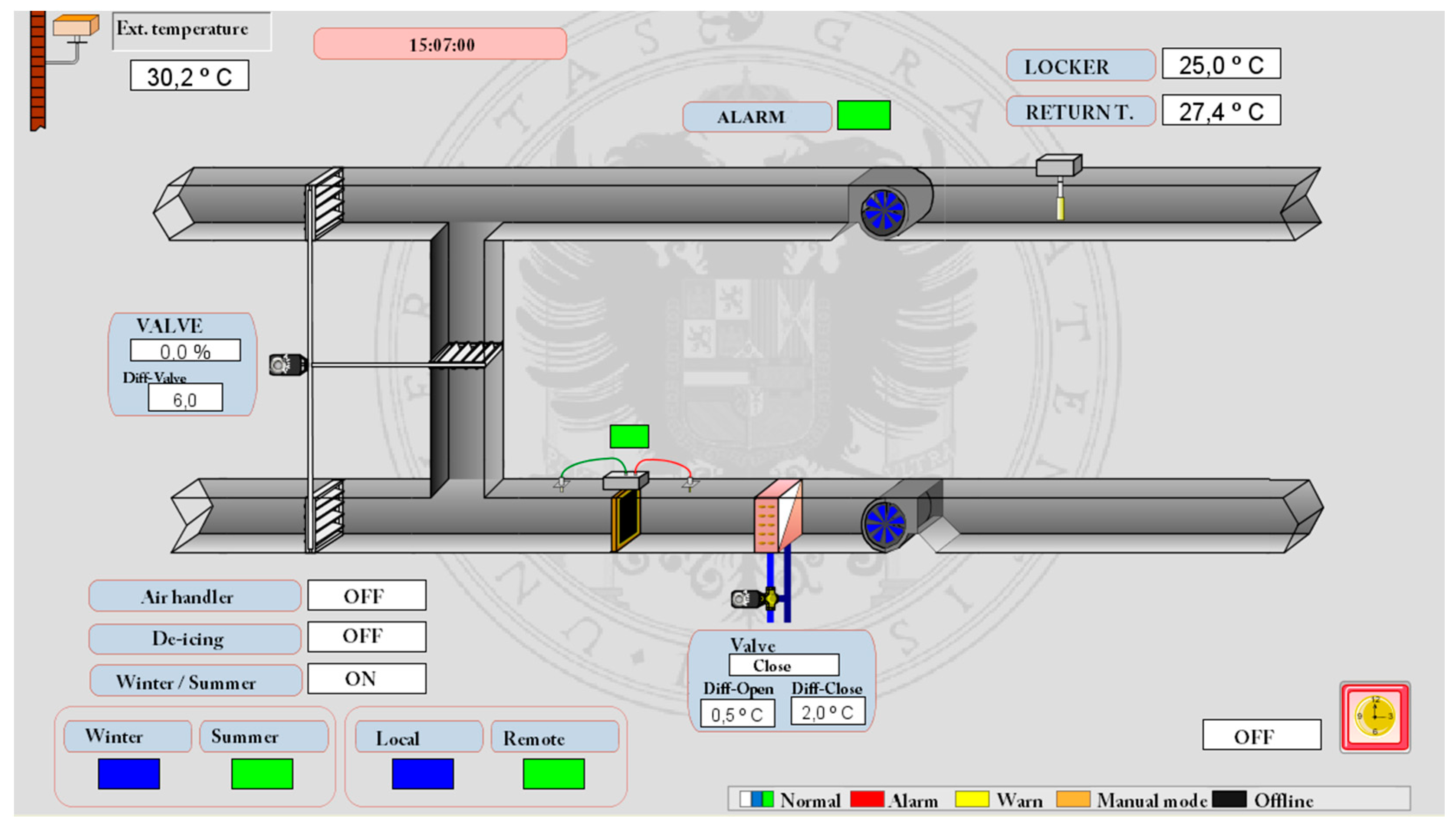
Regarding the temperature monitoring system, Figure 7 shows an example of a complete control ventilation system. This system senses external temperature and internal building temperature. It has several valves to control optimal air conditions, such as the temperature in degrees Celsius in the environment, which leads the system to close or open valves and, thus, introduce appropriate air into the system. One sensor indicates if there is any problem in the system, and another sensor is used to distinguish between summer and winter. Furthermore, there is a de-icing device, which is turned on when the system detects that the temperature is too low to prevent freezing during the winter.

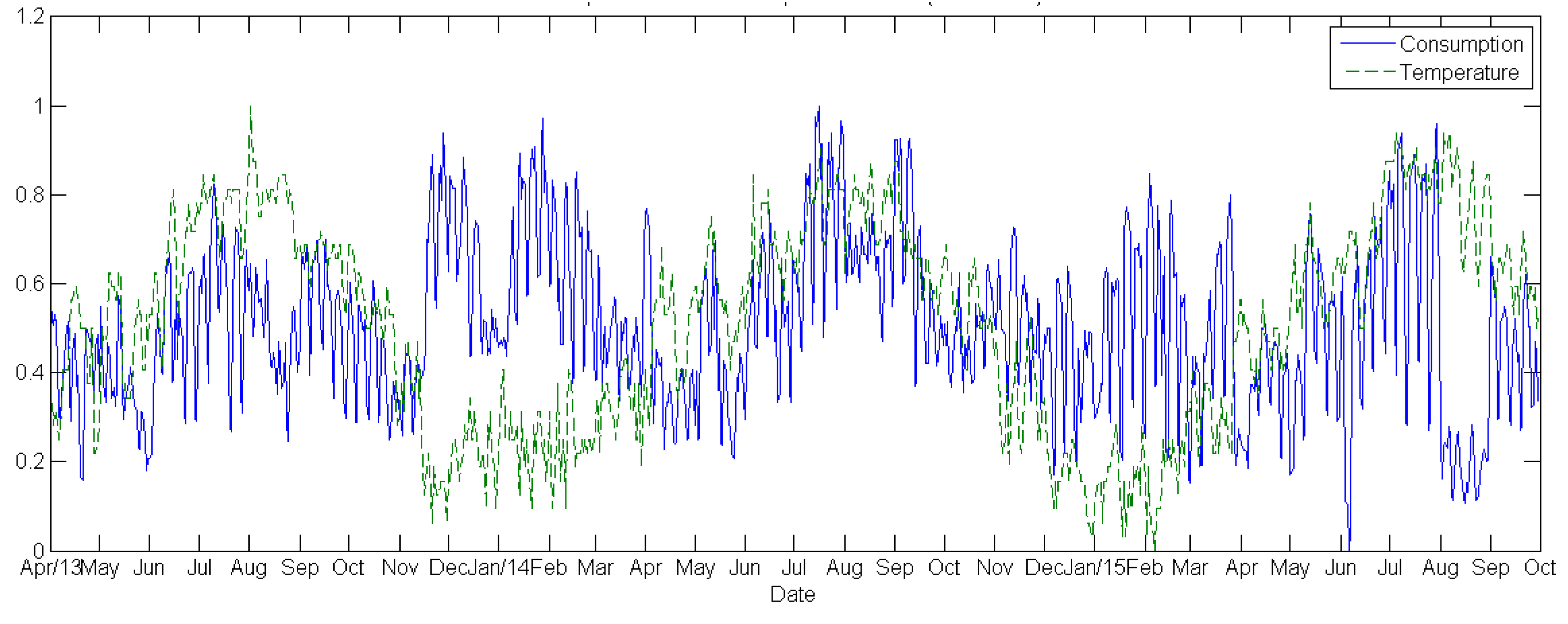
In this research paper, temperature will be a useful and distinctive characteristic because of its relation with energy consumption. These results will be discussed in more detail in the experimental section. It is reasonable to believe that if the temperature becomes too high or too low air conditioners will have more use. Figure 8 shows the consumption and the temperatures registered over time. Both time series have been normalized because they have different data measurement units. Temperature is in degrees Celsius and consumption is in kW. This figure illustrates interesting trends which have been described previously. For instance, low temperatures, such as those between December and February, have a high consumption and the air conditioners were used more during those dates.

5. Results

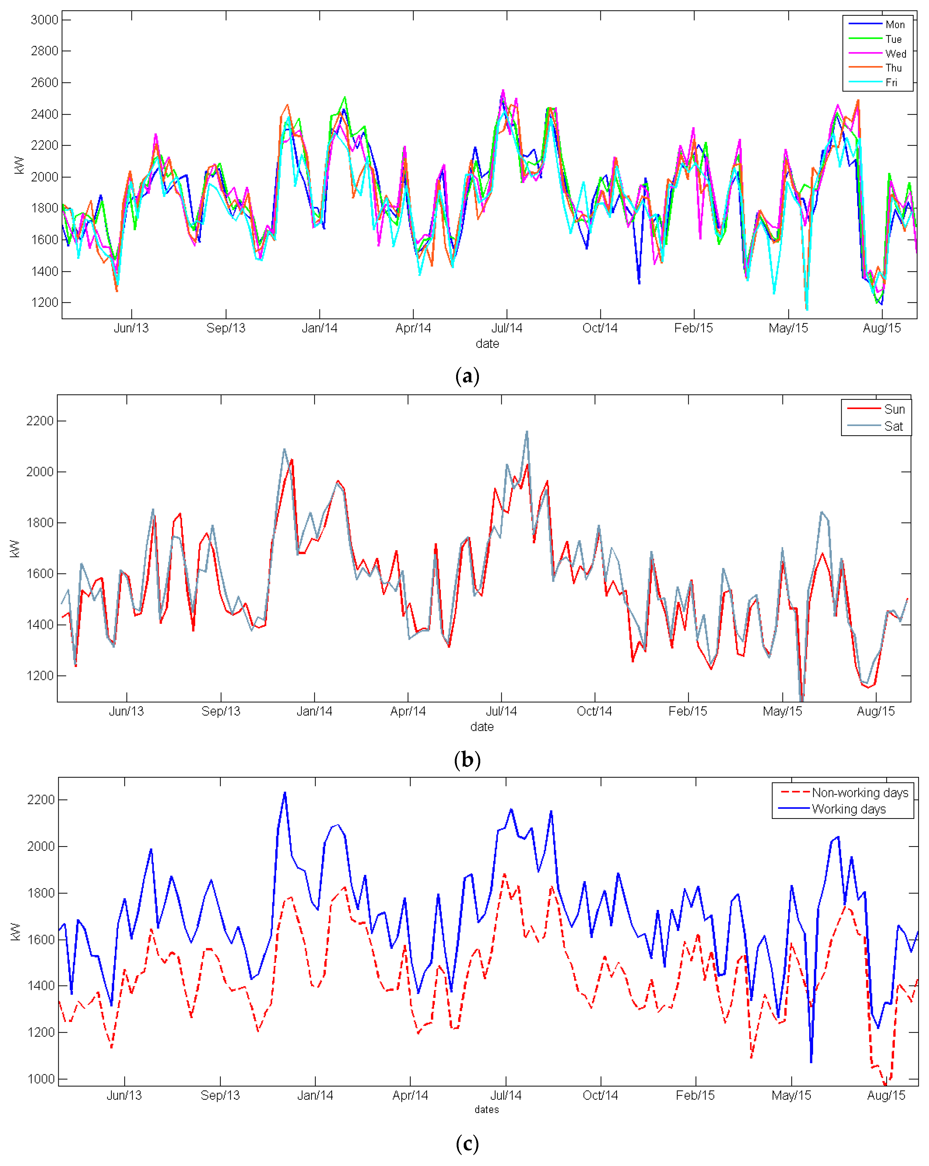
This section describes the entire series of tests performed and their experimental settings. Figure 9 shows the consumption of a sample building during a period of two years, including all week days. Figure 9a illustrates the building’s consumption during working days; and Figure 9b shows the consumption on Saturdays and Sundays. It is important to remark that the consumption is similar for days that are consecutive, both on the working and weekend days. Thus, the weekdays in the graph are almost indistinguishable from each other. Nevertheless, this behavior is very interesting and is useful to adapt the parameters of the forecasting models. In other words, one example of relevant information which can be mined of this data is if a week starts with an increase in consumption, the previous and next days will have the same behavior.

Figure 9a,b show similar behavior between the same types of day. Likewise, the behavior presents similarity between different types of days. On one hand, the increases and decreases in consumption have the same shape in the Figure 9c, although, as noted in the figure, consumption is almost always lower on non-working days.

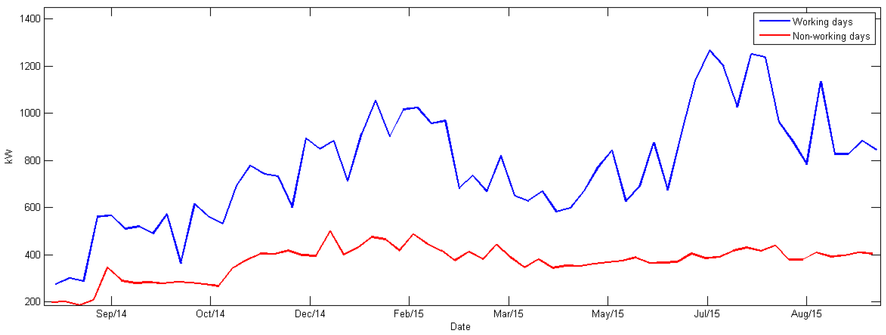
Unfortunately, this behavior is not the same for all buildings. Figure 10 shows consumption registered in another building on working and weekend days. This time, these two time-series follow two different progresses: non-working days and working days seem to follow a completely different trend depending on the building type. We are not able to establish a relation between these two behaviors according to the building use (offices, classrooms, data centers, research centers, etc.); the mining of the underlying data relations that produce these types of consumption will be a subject of further research. As a consequence, in the current study, we make no initial hypotheses about the data relationship between buildings.

According to this information and analysis, it is important to adjust the delay parameters of the ANN for each building separately, in order to obtain an accurate prediction model in each case. Delay parameters concern the number of days the model is going to use to perform the consumption prediction. In other words, the model is trained with the last $p$ days as delays. We have experimented and run 10 tests with ten different delays to find the most appropriate value for each building. Among these are: the day before ($p=1$); the complete last week ($p=7$); the last two weeks ($p=14$); and the last three weeks ($p=21$). To find the best delay, we set all parameters to a fixed value and modified the delay in a trial-and-error procedure to find the value that could provide the network with the best performance.

Table 1. MSE of the delay parameter obtained with the NAR model.

Consumption	Delays
	1	3	5	7	9	12	14	16	18	21
Building 1	5.80	2.50	2.28	2.13	2.06	2.02	2.01	2.03	2.22	2.05	Worst
Building 2	3.82	2.28	1.80	1.53	1.53	1.42	1.52	1.61	1.49	1.57	Best
Building 3	4.80	2.24	2.09	1.83	1.53	1.30	1.66	1.51	1.69	1.76
Building 4	4.87	2.68	2.16	1.78	1.95	1.85	1.72	1.75	1.82	1.83
Building 5	1.70	1.21	1.17	0.85	0.71	0.78	0.74	0.79	0.75	0.73
Building 6	2.95	1.75	1.08	0.80	0.62	0.81	0.80	0.78	0.85	0.88
Building 7	5.41	3.12	1.87	1.67	1.58	1.35	1.51	1.66	1.62	1.67
Building 8	3.29	1.97	1.59	1.08	0.94	1.06	1.08	1.09	1.03	1.02
Mean	4.08	2.22	1.76	1.46	1.37	1.32	1.38	1.40	1.43	1.44

Bold values: the best delay; crossed-out values: the worst error.

illustrates the average mean square error of 10 executions for each delay value and building, using the NAR model. From this table, we can acquire the best delay obtained for each building (marked as bold values). In all cases, the worst error is acquired with only 1 delay (marked as crossed-out values). The minimum delay required to get the most accurate prediction performance is nine days; although two buildings extend to two weeks to get the best result. From these results, conclusions can then be made relative to the delay information: a delay of between nine to 14 previous days is needed in order to obtain the best NAR forecasting model.

Once the delays have been set, the next step is to adjust the number of neurons needed to train the NAR network. In this case, the delay parameters have been set to a fixed value, obtained from the best MSE attained in Table 1. With these delays, we have run 10 different executions of each network configuration to find the average MSE of each setting, in order to find the best network structure for each energy consumption time series.

Table 2. MSE of the neurons parameter obtained with the NAR model.

Consumption	Neurons
	2	4	6	8	10	12	14	16	18	20
Building 1	2.27	1.83	1.82	1.87	2.10	2.20	2.13	2.08	2.14	2.15	Worst
Building 2	1.63	1.78	1.48	1.54	1.64	1.44	1.62	1.61	1.94	1.67	Best
Building 3	1.81	1.69	1.54	1.67	1.63	1.68	1.59	1.58	1.91	1.64
Building 4	1.78	1.90	1.75	1.73	1.70	1.90	1.85	1.77	1.93	1.87
Building 5	0.72	0.70	0.70	0.67	0.74	0.69	0.75	0.72	0.76	0.79
Building 6	0.75	0.78	0.85	0.77	0.74	0.64	0.76	0.80	0.90	0.87
Building 7	1.82	1.49	1.70	1.89	1.62	1.36	1.73	1.58	1.71	1.52
Building 8	1.20	1.10	0.96	0.96	0.93	1.00	0.95	1.02	0.94	1.03
Mean	1.49	1.41	1.35	1.39	1.39	1.36	1.42	1.40	1.53	1.44

Bold values: the best delay; crossed-out values: the worst error.

collects experiments with a different number of hidden neurons, ranging from 2 to 20. This experimentation is aimed at knowing the network structure that can provide the best performance. It emerges that more neurons result in a worse prediction, due to local optimum optimization results using the training algorithm, and also to overtraining. From Table 2, we conclude that the best average errors are obtained using between six and 12 neurons, depending on the building in question.

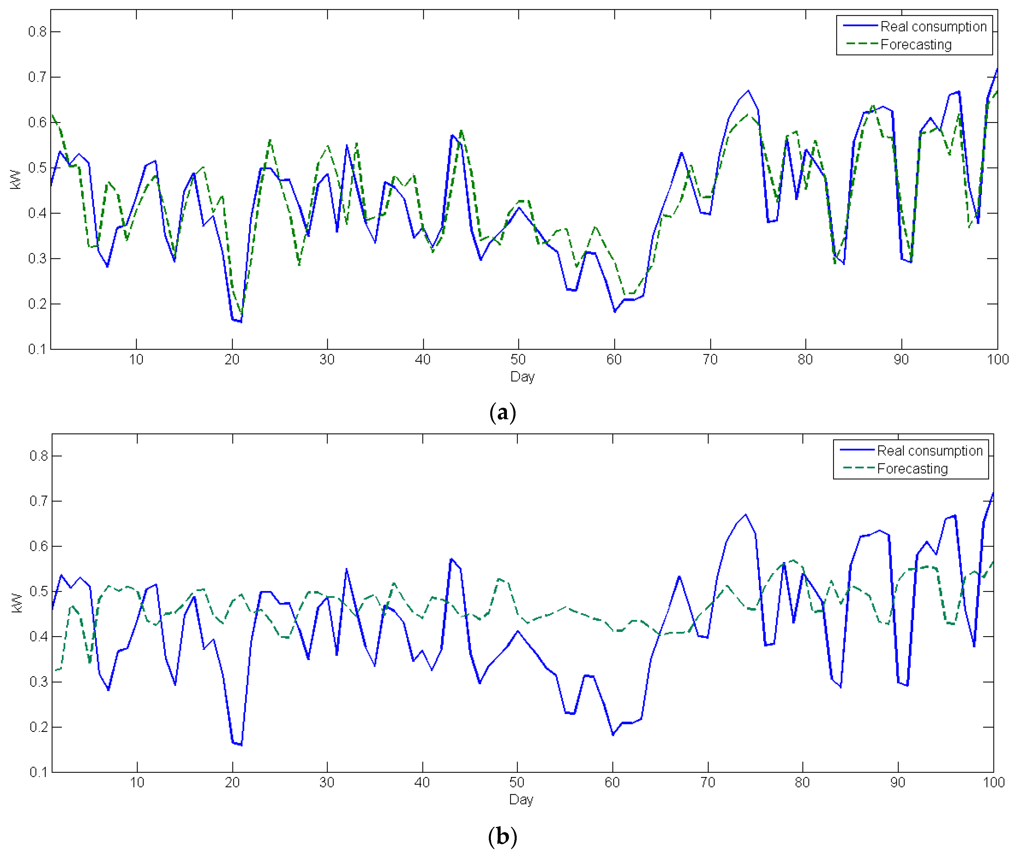
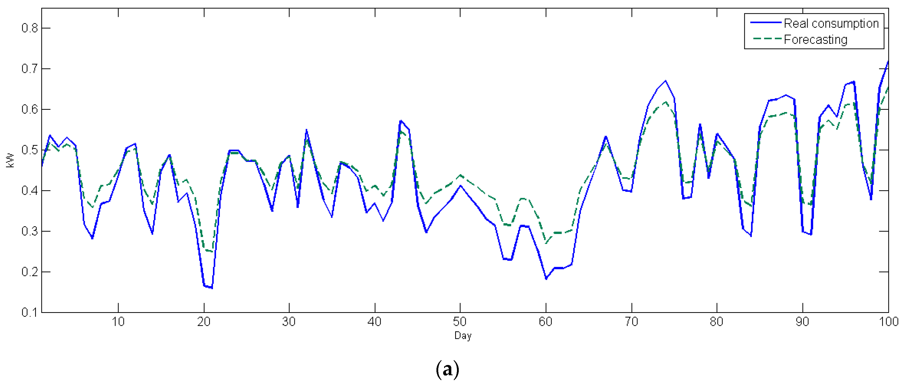
After this experimentation, we acquired the best NAR networks trained to predict the energy consumption of the eight buildings. Figure 11 shows an example of the prediction of energy consumption for Building 5, for a period of 100 days. This figure contains both the best and the worst trained networks in the 10 runs. Figure 11a presents the best forecasting curves captured, with a MSE of 0.68, and the second shows the worst forecasting, with a MSE of 2.23.

Since these experiments have been run using NAR models, the results have been obtained using consumption information only, without external data. NARX models allow the use of extra information that could be useful for the prediction. In this study, we use temperature data as an external variable.

For the experimentation with NARX, we followed the same methodology as with NAR models.

Table 3. MSE of the delay parameter obtained with the NARX model.

Consumption	Delay MSE
	1	3	5	7	9	12	14	16	18	21
Building 1	1.83	2.12	1.63	1.50	1.52	1.82	2.14	2.06	1.84	2.07	Worst
Building 2	1.77	1.69	1.45	1.39	1.53	1.48	1.44	1.40	1.58	1.59	Best
Building 3	1.59	1.47	1.51	1.35	1.58	1.46	1.55	1.90	1.66	1.76
Building 4	1.69	1.58	1.58	1.71	1.71	1.83	1.80	1.99	1.94	2.16
Building 5	0.91	0.79	0.76	0.79	0.83	0.87	0.90	0.93	0.95	1.01
Building 6	1.08	0.83	0.77	1.03	1.12	1.16	1.13	1.24	1.44	1.31
Building 7	1.33	1.44	1.17	1.27	1.36	1.35	1.71	1.54	1.57	1.65
Building 8	1.03	1.09	1.05	0.99	0.99	1.06	1.30	1.14	1.34	1.34
Mean	1.40	1.38	1.24	1.26	1.33	1.38	1.50	1.52	1.54	1.61

Bold values: the best delay; crossed-out values: the worst error.

shows the results regarding the delays required in order to obtain the best model. In this case, the best delay horizons are under one week, whereas the worst delay horizons are always over two weeks.

In the same way as was done for the NAR model,

Table 4. MSE of the neurons parameter obtained with the NARX model.

Consumption	Neurons MSE
	2	4	6	8	10	12	14	16	18	20
Building 1	1.70	1.33	1.66	1.88	1.70	1.73	1.70	1.59	1.69	1.86	Worst
Building 2	1.31	1.47	1.50	1.44	1.65	1.74	1.77	1.54	1.66	1.78	Best
Building 3	1.24	1.45	1.21	1.27	1.28	1.52	1.34	1.37	1.49	1.64
Building 4	1.45	1.74	1.63	1.70	1.85	1.77	1.40	1.62	1.71	1.80
Building 5	0.71	0.82	0.74	0.86	0.85	0.82	0.78	0.82	0.82	0.90
Building 6	0.79	0.87	0.84	0.85	1.08	0.94	1.01	1.03	1.00	1.10
Building 7	1.17	1.39	1.27	1.35	1.31	1.31	1.24	1.67	1.59	1.30
Building 8	0.88	1.05	1.03	1.01	1.01	1.06	1.08	1.11	1.12	1.01
Mean	1.16	1.27	1.24	1.30	1.34	1.36	1.29	1.34	1.39	1.42

Bold values: the best delay; crossed-out values: the worst error.

shows the results of the test with the number of hidden neurons. The best results achieved with the NARX model have been found with a fewer number of neurons since the best average MSE involve a minimum of two neurons in most of cases.

According to this information, we can conclude that using exogenous data may help to reduce the time horizon of past values to acquire an accurate prediction, but also that the network topology requires less computing units to perform the time series modelling. While the average number of neurons required by NAR to get the best forecasting is six, NARX uses an average of only two neurons.

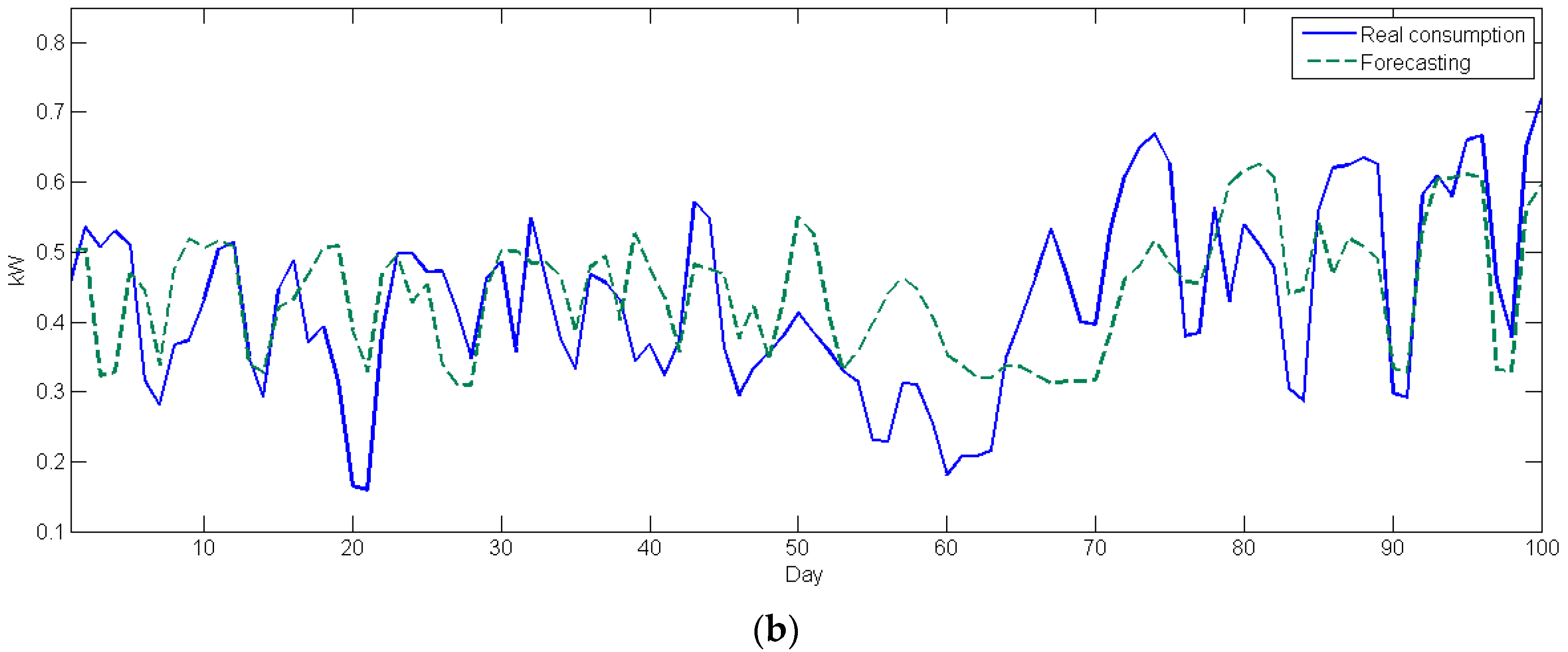
Figure 12 shows the forecasting curves using NARX models for the consumption data of Building 5. The best result obtained is plotted in Figure 12a, with a MSE of 0.66. Likewise, the worst prediction curve (Figure 12b) is better than NAR, with an MSE of 1.67. NARX models fit the consumption data better, due to the effect of exogenous data.

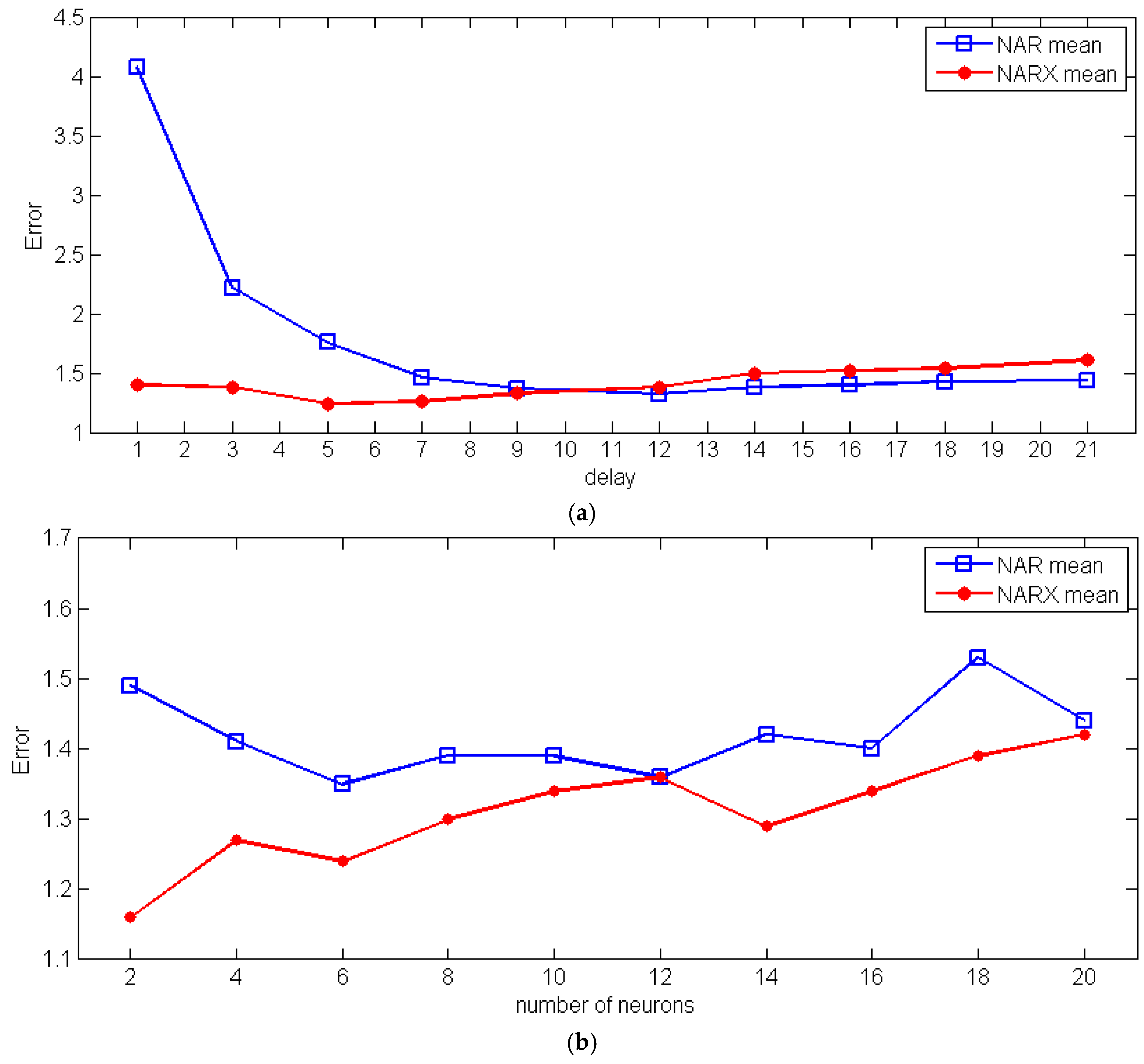
Finally, Figure 13 compares the means obtained with NAR and NARX networks in respect to the models’ complexity (number of hidden neurons). Both graphs demonstrate that NARX’s outcomes are better than NAR’s. The curve of MSE in the case of NARX network is below the NAR curve in the majority of cases, especially when the network complexity is simpler. The next section discusses all of the results and outcomes obtained from this experimentation.

6. Discussion

Our experimentation has focused on the comparison of neural network models for energy consumption forecasting, considering those cases where there are exogenous data available and those where there are not. Thus, the first issue to be taken into consideration is the availability of data, so that we can perform the model selection. The relative novelty of sensing technologies means that there are still buildings without automated management systems and, consequently, little information can be used. In these cases, the only information stored is the energy consumption. However, there is an increase in the installation and use of complex energy monitoring systems, which enables the possibility of using additional data to model the energy consumption. In the former case, only the consumption data can be used to make the prediction, whilst in the latter case we are able to include external information, such as weather conditions, to design a more accurate prediction model.

According to the analysis of results carried out in the previous section, it is important to draw attention to the significance of the delay parameter. The results collected in Table 1 and Table 3 show that each building’s consumption data requires its own delay parameter, and its value cannot be generalized to the whole building compound. This delay parameter is important because each set of buildings has different behavior, as is observed in Figure 9 and Figure 10. However, we have found that the use of exogenous data may help to reduce the time horizon of past values to be used for the prediction in all cases, since NARX requires fewer delays than NAR, therefore obtaining simpler prediction models.

The experimentation using NAR models demonstrates that this network architecture is useful when only energy consumption information is available, and can provide accurate mid-term predictions. This alternative can be used with a simple dataset containing consumption information only. Table 1 shows that a NAR model with little knowledge, such as one day of delay, is not enough to model the data and provides the worst results. In our dataset, a NAR model requires at least nine days of delay horizon to fit a good predictor. Including a larger delay horizon is not necessary to improve results, since the performance stabilizes after nine days in the delay parameter, according to the results of Figure 13a.

Regarding the network complexity, Figure 13b shows that a simple model with fewer neurons is not capable of modeling the time series complexity, but it also demonstrates that a large number of neurons provides unsuitable results due to local optima in the network parameters’ optimization process during the training stage. Indeed, the worst outcomes result from a large number of neurons.

Finally, the accuracy of these models provides a suitable prediction, as is shown in the sample of Figure 11a.

Regarding NARX neural networks experimentation, results show that the inclusion of simple external data, such as temperature, can help explain sudden changes in the trend of the consumption data and, therefore, obtain a more accurate prediction. For instance, during a hot summer week, if the weather remains constant, it is normal that the consumption is considered to be similar on all days of the week. In the NAR model these changes are not considered, but NARX can model them and use this information to improve the prediction accuracy.

As a consequence, the NARX model requires less past information than the NAR model to achieve an accurate prediction. According to Table 1 and Table 3, the number of delays required in the same dataset decreases abruptly from one model to another. The study of average MSE in respect to the delay horizon in Figure 13a also supports this analysis. The curve of NAR’s MSE regarding the delay parameter quickly decreases as the delays increase, yet these changes are not as radical in the NARX model. In this case, the exogenous temperature data help to model the energy consumption, so that fewer past consumption data are required for the prediction. Half of the outcomes provide the best results using the past five days as delay, and the rest using seven days.

With regard to the NARX model complexity, this approach only needs two neurons to get the best results in five buildings (Table 4). Although the consumption of Building 4 obtains the best MSE with 14 neurons, the second best results are obtained with two neurons. Similar results are drawn for the consumption data of Building 3, where the best results are obtained with six neurons and the second best results with two neurons. However, the consumption of Building 1 needs four neurons and no simpler model provides better results.

According to Figure 13b, the network complexity is always lower when using exogenous data. Since fewer delays are required to obtain the best prediction, fewer computing units (neurons) are needed in the network. When compared to the NAR model, NARX is able to obtain a better prediction accuracy using less historical data, and also with less model complexity. This analysis is supported by Figure 12, where it is shown that the prediction obtained with the NARX model adjusts considerably well to the curve of the real data, with respect to the NAR model.

In summary, Figure 13 provides clear data about the benefits and costs of the proposed network models. The NAR model is a good option when no exogenous information is available. It works with a simpler dataset, but requires a more complex model to get a good predictor. On the other hand, the NARX model can work with external information, and this alternative allows us to feed the model with additional data to obtain simpler predictors. The NAR neural network needs a higher delay horizon and more neurons to adjust a good model; NARX takes advantage of exogenous information to achieve better outcomes with less historical data. Figure 13 shows that the NARX model improves the results of the NAR network; in fact, the worst outcomes achieved by NARX are close to the best results of the NAR in the majority of cases.

As a final remark,

Table 5. Summary of NAR and NARX network performance (MSE) in all buildings.

Consumption	NAR	NARX
Building 1	1.82	1.33
Building 2	1.44	1.31
Building 3	1.54	1.21
Building 4	1.70	1.40
Building 5	0.67	0.71
Building 6	0.64	0.79
Building 7	1.36	1.17
Building 8	0.93	0.88
Mean	1,26	1,10

summarizes the results obtained for the prediction of all buildings, using NAR (column 2) and NARX networks (column 3). According to these results, the use of exogenous data may provide better results in most cases, in terms of prediction accuracy. However, if no external data is available, only the energy consumption might be used to obtain accurate predictions.

7. Conclusions

In this study we have provided a methodology to predict energy consumption in a set of public buildings using neural networks. In our approach, we assume that each building is equipped with an automation system containing energy consumption sensors that store consumption data in a shared database, but we also perform experimentation considering that other external data, such as temperature, are available. Using the sensor data in this database, we applied data pre-processing techniques to transform and normalize the data and remove the noise. After that, we tested different prediction models coming from the neural network area: NAR and NARX. Although both approaches provide suitable prediction accuracy, NARX networks furnish a better performance thanks to the exogenous data. Other advantages of using these exogenous data concern the decrease in the network complexity and the amount of historical data or delays to be used in the forecasting.

According to the dataset, we have discovered that building consumptions at the UGR can be aggregated into two main categories whose main feature is the similarity/dissimilarity of the energy consumption during the working and weekend days. Having knowledge of relations between the buildings’ consumption in advance, and the features that explain these relations, could enable us to use the consumption data of one or more buildings on a campus as exogenous data to predict the energy consumption of the remaining buildings—using the hypothesis that there is a correlation between those data, as the analysis of Figure 9 suggests. In a future piece of research, we will test these assumptions to study the increase in the prediction accuracy.

On the other hand, future research will be also targeted at developing an automatic procedure to find time relations in the energy consumption of the buildings, using data mining techniques to cluster data. We believe that the study of the effect of intra-cluster and inter-cluster relations, and information fusion techniques, will be key aspects to building decision-support systems for energy efficiency.