1. Introduction
Natural gas has the fastest growing consumption rates among clean energy resources in the world. It is considered a common resource and is used in different sectors such as heating, electricity generation, transportation, cooking, and cooling. Large investments are needed for forwarding, transporting and using natural gas. Some factors that affect these investments are whether the investment matches the consumption amount or how much air pollution occurs. Contracts have been made between various countries for natural gas supply whereby usage started at the beginning of the 1990s and demand has rapidly increased since then [
1,
2]. These contracts are mainly take-or-pay type contracts, focusing on estimating long-term natural gas consumption. One of the characteristics of take-or-pay contracts is that for lower consumption than estimated the price of estimated consumption must still be paid. However, for higher consumption then estimated, reducing the gas supply by slightly closing the valve or paying an extra price per unit m
3 occurs. In order to avoid these situations and reduce economic and social losses, demand forecasting with some minimum acceptable error should be used. Country governments should have preliminary information on regional consumption levels for demand forecasting. The main objective of gathering the preliminary information is that regional consumers use natural gas for various reasons and together they form a country’s consumption capacity. For instance, large factories use natural gas for electricity generation and manufacturing. These factories consume similar amounts both in winter and summer seasons, so they mostly show stationary behavior. Likewise, as long as there is no failure, daily high consumption of electricity generation plants depending on electricity generation staying at the same levels. Besides high consumption factories, organizations and plants, there are low consuming corporations and residential consumers as well. Their consumption patterns are mainly affected by seasonal variations. For instance, consumption levels decrease in the summer season and noticeably increase in the winter period. Even if each region in the country has different consumption levels, low consuming consumers always have a critical amount of natural gas consumption at the national level. Since natural gas unit costs of these consumers need extra investment costs, their unit m
3 charges are higher compared to the high consumption sectors. Seasonal influences (change in consumption behavior) and high unit costs have made these consumers more important. Our case study is based on a city’s consumption in Turkey and this situation is also applied to cities in Turkey. Seasonally affected consumption behaviors of city consumers have an impact on the natural gas market in Turkey.
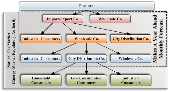
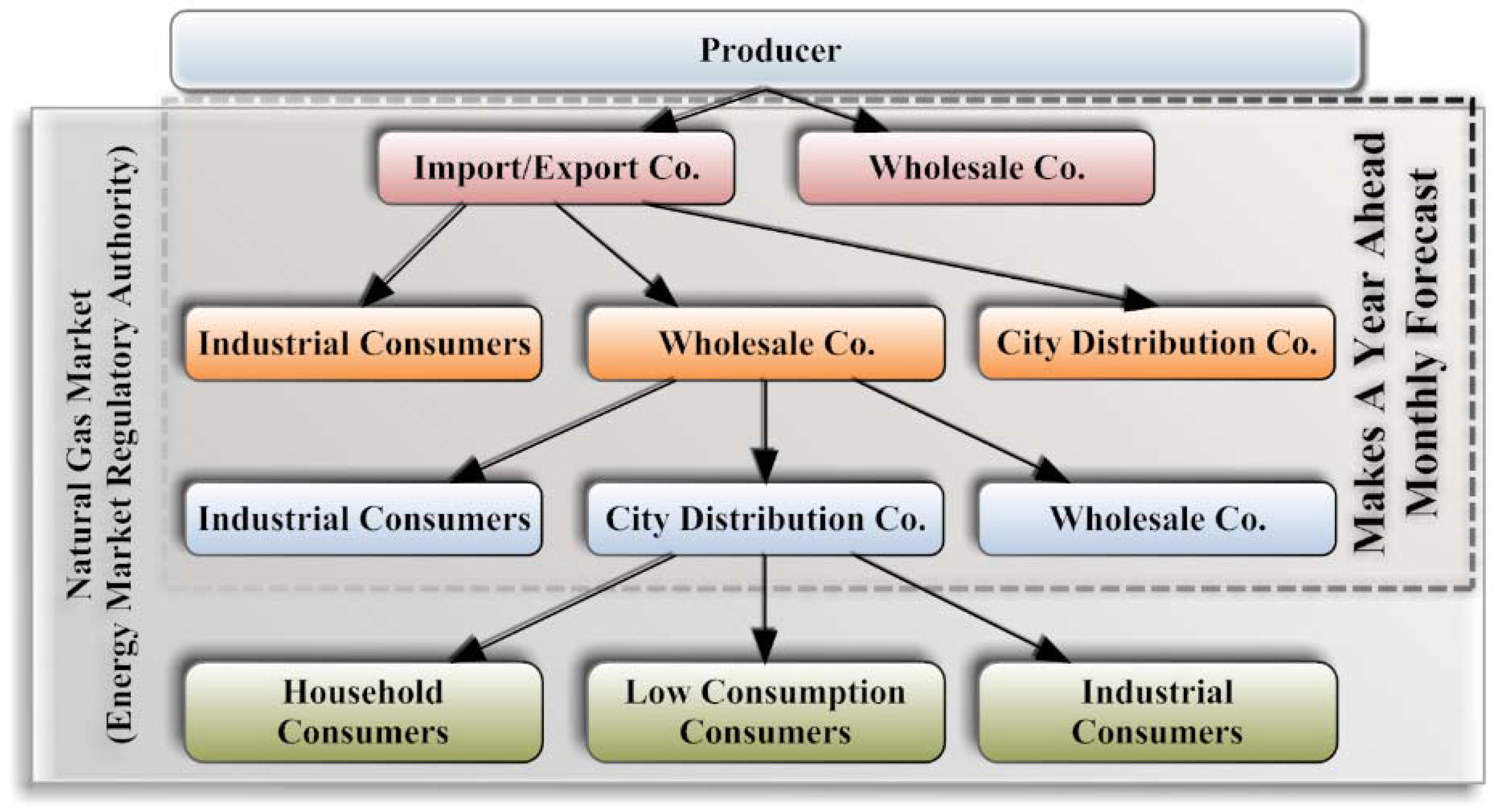
The natural gas market in Turkey is shown in
Figure 1. The companies placed on dotted lines perform an annual forecast based on regulations [
3]. The producers are generally outside Turkey [
4]. Import/export and wholesale companies could import natural gas to Turkey through pipelines or as liquid natural gas (LNG). At each level except the bottom, companies report their year-ahead forecasts in a hierarchical manner to the companies that have a contract. Finally, import or wholesale companies make a final estimation using bottom-up collected data. Each month, these forecasts are checked and if the mean absolute percent error is higher than 10%, penalties occur [
3]. The natural gas market is inspected by the Energy Market Regulatory Authority (EMRA, known by its Turkish acronym EPDK) and controlled by the Petroleum Pipeline Corporation (PPC, known as BOTAS). According to the EMRA report, in 2014, 49.262 billion m
3 natural gas was imported by nine long-term and two spot (LNG) import licensed entities [
4]. In the same report, it is stated that 7.281 billion m
3 of LNG was imported, which equals 14.78% of total imports. At the national level, the household ratio of consumption is nearly 20% of total consumption [
4]. This consumption amount is noticeably high, affecting penalties, and it is forecasted based on the bottom part of the market, from the residential/and small commercial end users who are subscribers of the City Distribution Company. As mentioned in the report, the sum of household and low consumption consumers comprises nearly 26% of total consumption at the national level [
4]. Therefore, the main objective of this application paper is to show the possibility of monthly forecasting natural gas demand for household and low consumption consumers by applying well-known univariate methods in the literature at the city level. Thus, it is expected that a low error rate and local error-free prediction results will be obtained.
The rest of the paper is organized as follows: related studies are presented in
Section 2. The data and theoretical description of methods are described in
Section 3.
Section 4 gives detailed information about modeling, definitions, scenario analysis and error benchmarks.
Section 5 presents pre-forecasting steps and
Section 6 shows the forecasting results and discussion. The key findings and next studies are given at the end of the paper as conclusions in
Section 7.
2. Related Work
Time series forecasting is an important area of forecasting in which past observations of the same variable area are collected and analyzed to develop a model describing the underlying relationship [
5]. Natural gas consumption predictions are being made with several approaches in different fields. These studies can be investigated as daily, monthly, national level, regional level, residential area, industrial area, use of an independent variable and no use of an independent variable.
In the first group, publications can be divided according to the use of timeframes which apply the time series method in daily periods [
6,
7,
8,
9,
10,
11,
12,
13,
14,
15,
16,
17,
18,
19] and monthly periods [
20,
21,
22,
23,
24]. In the second group, publications can be grouped as regional [
8,
9,
10,
11,
12,
15,
18,
19,
21,
22,
23,
24] or national [
6,
7,
13,
14,
20,
24,
25,
26,
27,
28,
29,
30,
31] consumptions are investigated. In the third group, papers are investigated by consumer types. This group includes household consumers [
6,
7,
8,
9,
10,
11,
12], commercial consumers [
11,
13,
25] and consumers where all consumption sectors are included [
14,
15,
16,
17,
18,
24,
25,
26,
27,
28,
29,
30,
31]. In the fourth group, where studies are categorized by data used, papers are divided with respect to the use of only consumption data using univariate approaches [
28,
29,
30,
31] or independent variable [
6,
7,
8,
9,
10,
11,
12,
13,
14,
15,
16,
17,
18,
20,
22,
23,
24,
25,
26,
27] included studies. Investigation of these studies showed that, mostly independent variable included regional-based natural gas consumption prediction is done. The summary of this research is published by Soldo [
32].
Univariate techniques have a broad usage area in time series forecasting. Ediger et al. used autoregressive moving average (ARIMA), seasonal ARIMA (SARIMA) and comparative regression techniques to forecast the production of fossil fuel sources in Turkey, which include natural gas [
33]. They made annual forecasts from 2004 to 2038 and used different regression types such as linear, logarithmic, inverse, quadratic, cubic, compound, power, growth, exponential, and logistic. They concluded that ARIMA is a suitable technique for natural gas consumption. Gutiérrez et al. used the Gompertz-type innovation diffusion process as a stochastic growth model to forecast annual natural gas in Spain from 1973 to 1997 [
29]. They compared the results between 1998 and 2000 with stochastic logistic innovation modelling and the Gompertz model was found to be more suitable. Ma and Wu studied China’s annual natural gas consumption and production prediction with the Grey model. They used data from 1990 to 2003 and generated forecasts for 2004 to 2007 [
30]. In a comparison between the Grey model (with one variable and rank 1 differential equation—GM(1,1)) and Grey-Markov model, the Grey-Markov gave better results. Xie and Li also used the Grey model to predict China’s annual natural gas forecasting. Unlike Ma and Wu, they used a genetic algorithm for optimizing the GM(1,1) model [
31]. They used data from 1996 to 2002 and predict for the forecast range of 2003 to 2005. Here, genetic optimization performed better results. In the literature, only Liu and Lin studied forecasting monthly natural gas [
34]. Their research is on a national level, and they made predictions on monthly and quarterly periods. They formed ARIMAX (ARIMA with eXogenous) models by adding temperature and price into ARIMA models.
Univariate statistical forecasting could also be also applied in other sections of the energy sector such as electrical, water, solar, wind etc. Yalcintas et al. studied water management through demand and supply forecasting for Istanbul city [
35]. They applied ARIMA to forecast annual demand 2015–2018 by using data from 2006 to 2014 and suggested that sustainable management of water can be achieved by reducing residential water use through the use of water efficient technologies. Gelažanskas and Gamage used time series seasonal decomposition, exponential smoothing and SARIMA methods for predicting hot water demand [
36]. They found that the most significant part in the accuracy of forecasting is the seasonal decomposition method of the time series. Prema and Rao forecasted wind speed using time series decomposition, exponential smoothing and back propagation neural networks [
37]. They observed that decomposition of time series and ARIMA methods gave more accurate results. The ARIMA method has been frequently used for daily and hourly load prediction of electricity consumption. Research on time series applying electricity prediction is presented as a survey [
38]. It is observed that ARIMA is one of the most used linear prediction techniques. For instance, Wang et al. studied electricity price estimation with Winters’ exponential smoothing and SARIMA methods [
39].
5. Case Study
The case study models low consuming commercial and residential consumers’ natural gas consumption by seasonal univariate statistical methods (time series decomposition, Holt-Winters exponential smoothing, ARIMA, SARIMA). The natural gas consumption data is collected from the city of Sakarya, Turkey. Industrial hourly consumption data (102 users) was summarized as monthly and another 12 industrial subscribers’ consumption was prepared from manually billed invoices. The consumption of RMS-A is prepared between the years 2011–2014 (48 month-long) and this data was later divided into two parts. In the first part, 2011–2013 (36 month-long) data is used for monthly forecasts, and in the second part, 2014 (12 month-long) data. In the next section, the evaluation and comparison of results will be presented for all series and for 2014 separately. The error and estimation accuracy will be also investigated with MAPE and Ṙ².
Hereafter, time series decomposition, Holt-Winters exponential smoothing and autoregressive integrated moving average are referred to as “D”, “W” and “ARIMA”, respectively. Each applied method has its own sub-techniques. These three methods are preferred as they all include the seasonality effect.
The time series decomposition method can be additive or multiplicative as shown in
Table 1. If the values increase or decrease proportionally over time, the “multiplicative model” gives better results. However, if values increase or decrease additively over time the “additive model” gives better results. This study applies both additive and multiplicative models in order to show which technique has more influence on natural gas prediction. The decomposition process of this method can contain both trend and seasonality or only the seasonality estimation method. Consumptions that increase during winter and decrease during summer indicate the seasonality effect. Therefore, all decomposition methods contain seasonality. Besides seasonality, this research investigates both trends and seasonality included situations to determine the trend effect on consumption. Thus, two situations (additive/multiplicative or trend/seasonal) can generate up to four different estimations. These four techniques can be easily computed with simple mathematical operations on spreadsheet software.
Holt-Winters Exponential Smoothing is the second method used. This approach can be additive or multiplicative as well (
Table 2). The determination of α, β and γ parameters is important in this method. Before the determination step, default values for α, β and γ are taken as 0.2 as stated in [
51]. However, these values will not give the best results. In order to obtain the best result, they should be optimized. Various methods are used in convergence. In this work, ordinary least squares (OLS) is applied as the convergence technique. The convergence value is 10
−7 and iteration number is 500,000. In abbreviation, coefficients are divided by ”c” char. The left side of “c” is the Holt-Winters method such as “A” for additive and “M” for multiplicative. The right side of “c” is parameters. If default values are taken, it is 0.2 or else it is written as “Opt” in generally. This technique can be implemented on spreadsheet software with programming experience.
Other forecasting techniques used in the study are ARIMA and SARIMA methods. The stationarity of the series is investigated by these methods. In this respect, necessary conversion operations are done and the series is stationarized. In order to stationarize the series, differentiation is applied to the ARIMA method. On this new stationary series, particular parameters are determined such as AR, MA, seasonal AR (SAR) and seasonal MA (SMA). Data generated by taking the difference can be described as:
Secondary difference; Δ²log(Consumption); I(2)1 or ARIMA(0,2,0)1.
Primary seasonal difference; Δ₁₂log(Consumption); I(0)1(1) or ARIMA(0,0,0)1(0,1,0)12.
Primary difference and primary seasonal difference; Δ₁₂,₁log(Consumption); I(1)1(1) or ARIMA(0,1,0)1(0,1,0)12.
Equations are formed containing these parameters and later estimations are done.
Natural gas consumption values are related to weather conditions, the number of consumers and calendar effects. Eventually, the consumption is formed by these facts. The main objective of this paper is to show the possibility of monthly forecasting natural gas demand on the city level by performing well-known univariate methods in the literature. Thus, the low error rate and local error-free prediction results will be obtained.
6. Pre-Forecast
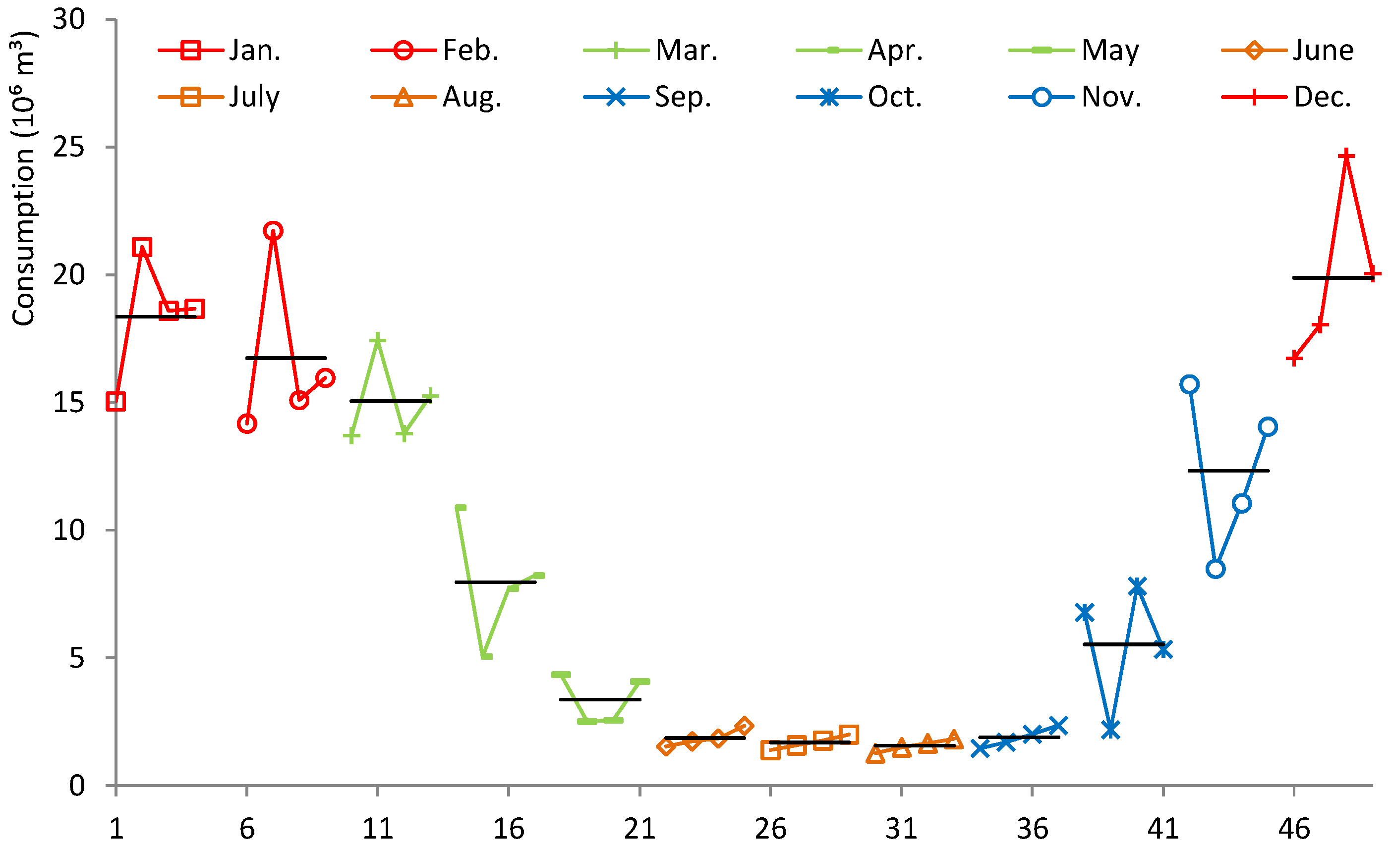
Natural gas consumption changes depend on weather conditions. Seasonal impact mainly causes the weather change. Thus, natural gas consumption is influenced by seasonal facts (
Figure 2). In D and W methods, seasonality is mandatory in a series. In this way, forecasting is more accurate with the help of seasonal effects. On the contrary, ARIMA and SARIMA methods require stationarity in a series. In other words, seasonality should not exist in a series. Since stationarity is an important fact, preprocesses need to be accomplished. The first step is setting the T value to 1. This process takes the logarithm of a series. There is no difference between the series and logarithm. Only the range of the series is narrowed.
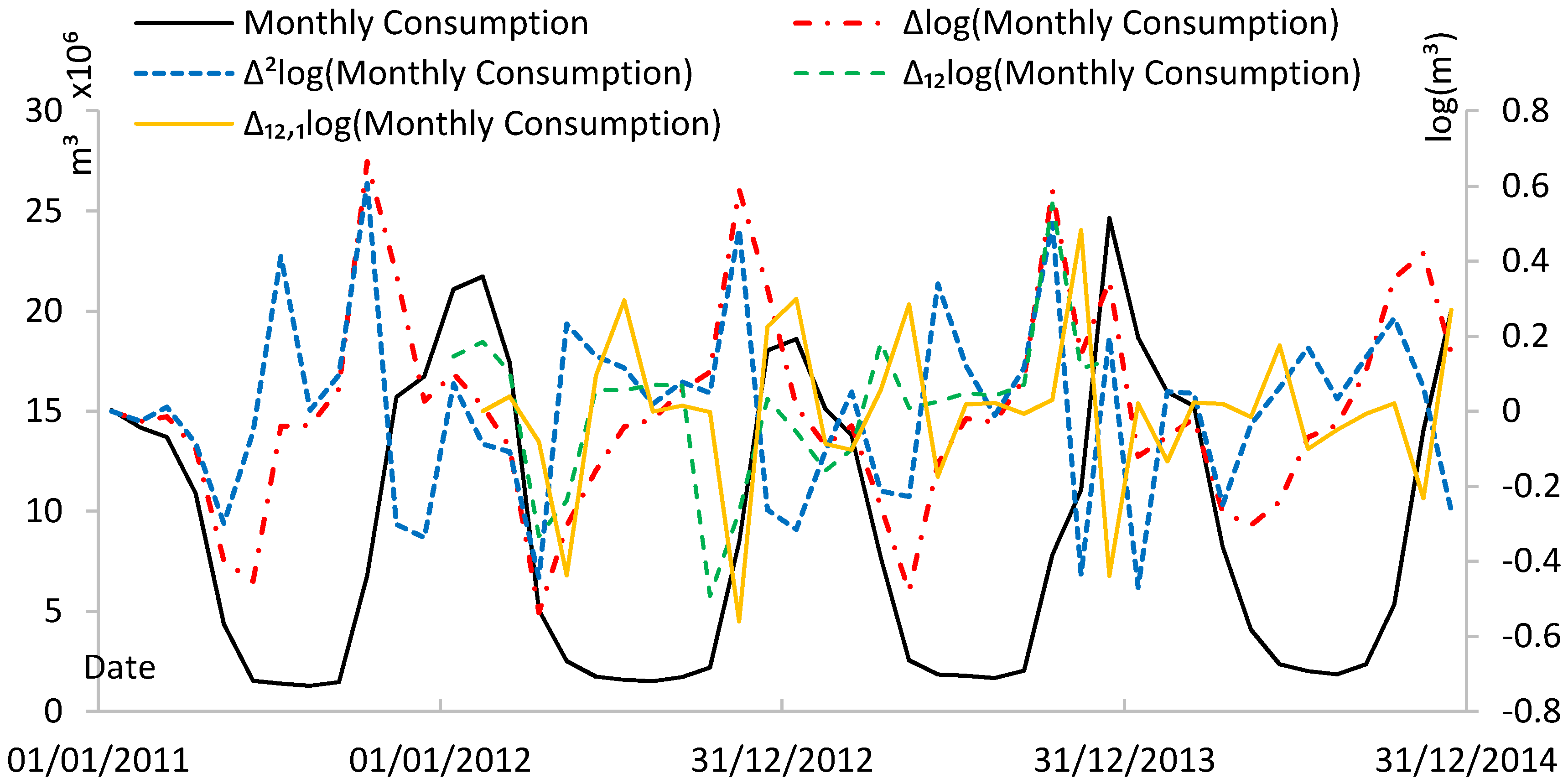
In order to stationarize the series, differentiation processes should be completed. The differentiation operation is represented with the “Δ” operant. The difference between the series itself and the previous value of it is called the first difference, and it is presented singly. When the differentiation is applied again to the differentiated series, the secondary difference is generated and it is denoted as Δ
2. The seasonality impact takes place on 12-month data in this study. Therefore, the seasonal difference of a series is shown as Δ
12. Both the seasonality and primary difference included series is shown as a Δ
12,1. This representation expresses that first seasonal difference, and the next primary difference is performed. In
Figure 3, consumption is presented on the left axis and logarithmic values are presented on the right axis of the graph. Results show that consumption series and logarithmic primary difference series are not stationarized. Other differentiation processes applied to the logarithmic series have stationarity.
Descriptive statistics in
Table 3 indicate that the log operation exposes consumption values between 6.108 and 7.392 on an average of 6.757 and standard deviation of 0.443. The mean of the first differentiated series is around zero and its standard deviation reduces by half according to the log(consumption) series. The second differentiated, seasonal differentiated and both seasonal and non-seasonal differentiated log series have a zero mean and reduced their standard deviations.
Even though stationarity can be seen visually (
Figure 3), the stationarity of a series is examined by ADF and PP tests [
54,
55,
58].
Table 4 shows probability values of the prepared series on ADF and PP tests. The tests basically investigate the existence of the unit root. This existence proves the series is not stationary. According to this, the hypothesis is prepared. Hypothesis H
0 defines that there is a unit root in a series while the alternative hypothesis shows there is not a unit root, meaning the series is stationary. In this computation, the significance degree of the
p probability value is taken as 0.05. If the
p value is less than 0.05, then the series is called stationary. Three situations of unit root tests are represented in the table, which are no constant and no trend, only constant, constant and trend. For these three situations, unit root tests are performed. “C” value in the table represents a constant in the equation, while “T” represents the trend. Regarding the outcome of the tests, ADF and PP tests show that all series are stationary except the raw consumption series.
Another way used to determine the stationarity of a series is analyzing ACF and PACF graphs. The ACF graph is demonstrated as an autocorrelogram and PACF is demonstrated as a partial autocorreglogram (
Figure 4). Depending on lags, correlograms vary between −1 and 1, and the significance degree of the relationship between the variable and its history is shown with a dotted line. The area above the dotted line is accepted as a significant relation [
41,
42]. When ACF and PACF are analysed, it is seen that seasonal patterns of a 12-month series of Consumption and Δlog(Consumption) consumptions are noteworthy in ACF graphs. Although ADF and PP test results show stationarity, because of the seasonal patterns of these series, it is not appropriate to use them in forecasting. The Δ²log(Consumption), Δ₁₂log(Consumption) and Δ₁₂,₁log(Consumption) series do not have seasonal patterns. Thus, the ARIMA method can be easily applied to the generated series. It is observed that the autocorrelograms and partial autocorrelograms of these three series have a relation in the 12th month. The seasonality of the series can be seen by this way. The AR, MA coefficients in the non-seasonal and the seasonal parts are used between zero to three for finding the optimum forecast results. Different ARIMA models (256) were prepared and the forecast results are examined.
The equivalents of differentiation operations of ARIMA and SARIMA methods are called “I” values. Log of differentiate and seasonal differentiate are formulated as ARIMA(0,1,0)1(0,1,0)12 or I(1)1(1)12.
7. Results and Discussion
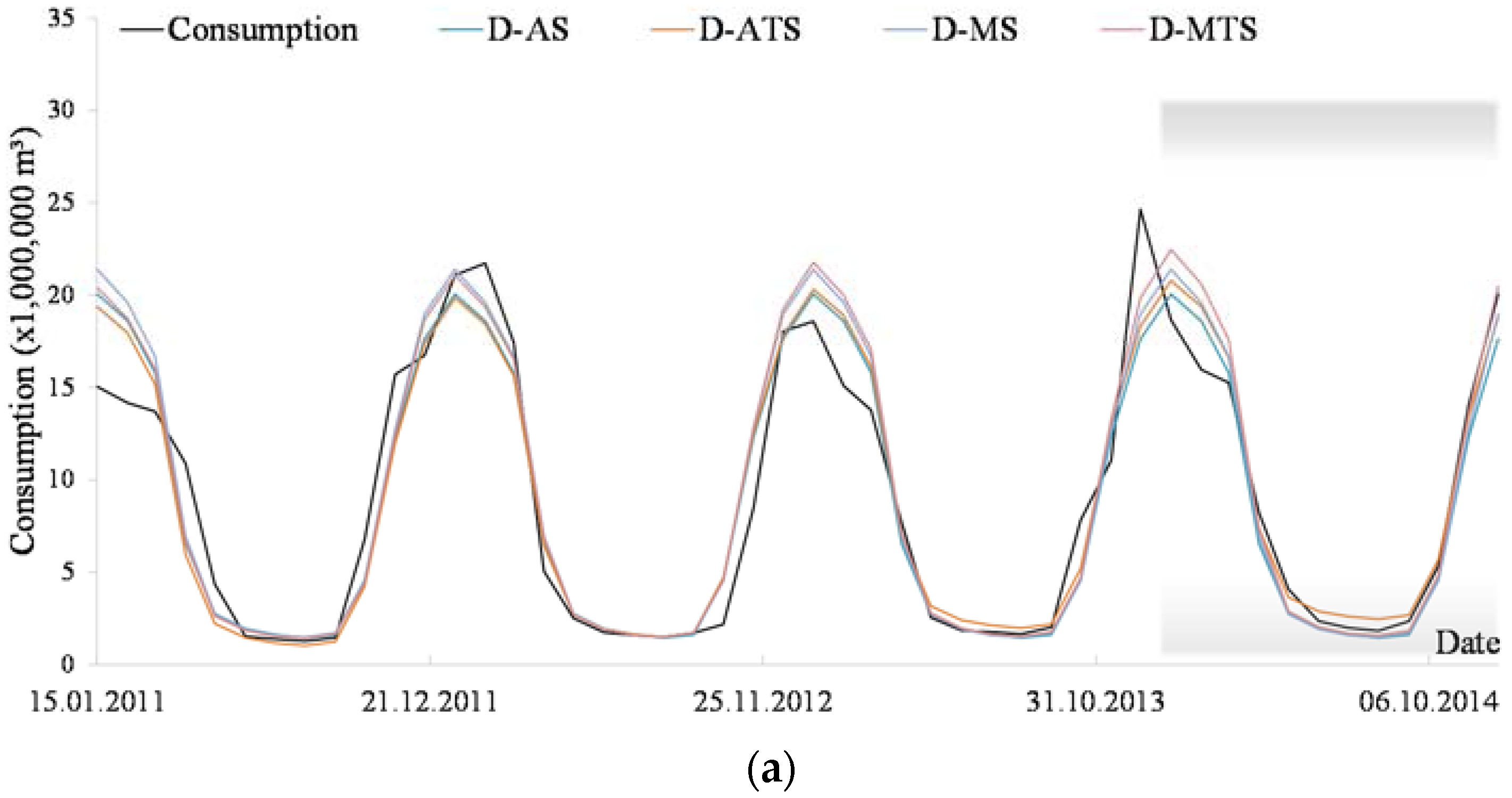
The forecast results are shown based on the method in
Figure 5. The year 2014 is shown in grey and a transparent box in graphs. In this way, the difference between the fitted historical data and the forecast can be easily seen.
For the decomposition model, the first method in the graph, at the beginning of 2014, the consumption and forecast difference is considerably large. However, this difference decreases gradually by the end of the year. Ṙ² and MAPE values for D-AS, D-ATS, D-MS, D-MTS are 0.907, 0.910, 0.909, 0.915 and 19%, 20%, 20%, 19%, respectively. It is clearly seen that high consumption in January affected forecasting in 2014. Even though spring and autumn seasons are difficult parts of the forecast because of climate changes, the decomposition forecast is well fitted here. The best outcome for 2014 is 15% MAPE at additive trend seasonal decomposition.
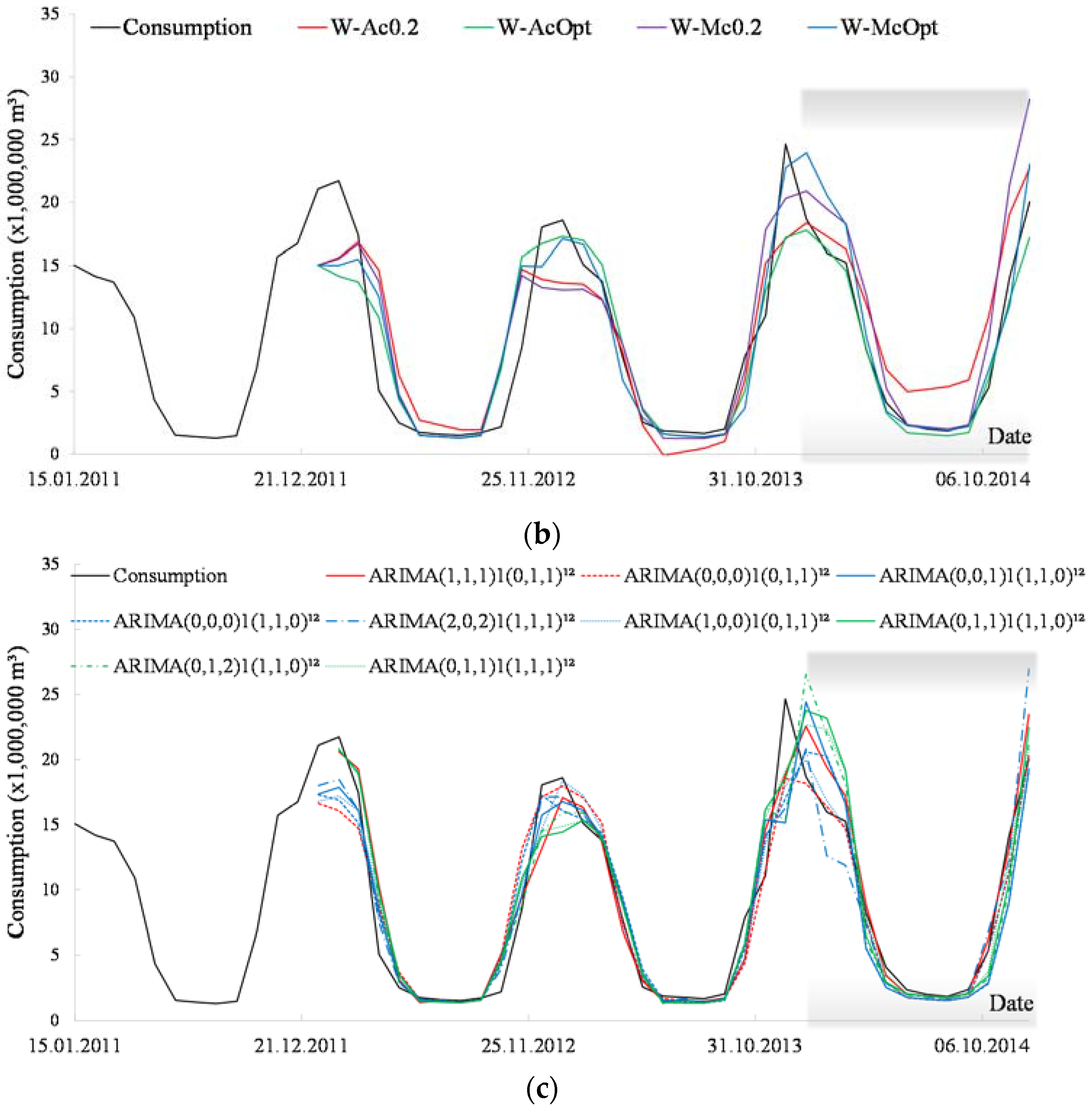
Holt-Winters exponential smoothing is applied with two sub-models, additive and multiplicative. Both sub-models’ coefficients are taken as 0.2 in the first study of the Holt-Winters model. After gathering results, the second study coefficients of the model are calculated with least square regression to find the optimized solution. The first study gives a weaker estimation than the optimized coefficients. Considering the additive and multiplicative models, the multiplicative models generate higher estimation values than additive models. The major reason behind this outcome is that the seasonal impact in the Holt-Winters method increases multiplicatively. Although additive stays at similar levels, the consumption forecast rises steadily with the multiplicative influence. Another point is that the Holt-Winters method has negative value estimations. Since parameters are taken as 0.2, the June 2013 consumption is around −95 × 10
3 m
3 (
Figure 5b). Since the estimation values cannot be negative, it can be evidently seen that the parameter selection is important. The optimized α, β, γ parameters are 0, 0.01, 0.375 and 0.15, 0, 0.74 for the additive and multiplicative methods, respectively. However in the Holt-Winters method, the optimized parameters α and β are very close to zero. Parameter γ is on average above 0.5, such that it proves the seasonal influence on the series, clearly.
Table 5 presents the results based on the data range and methodology. In cases where parameters are not optimized according to the optimized situation, (α, β, γ = 0.2) MAPE values are high and Ṙ² values are low (
Table 5). Non-optimized results present worse performance. For optimized results, however, the additive method has better outcomes than the multiplicative method, both on the entire series and the 2014 estimation. The lowest MAPE over the 2011–2014 period with the additive method is 28.81% and the highest Ṙ² value is 0.846. In 2014, the lowest MAPE is 14.01% while the highest Ṙ² is 0.983. The additive methodology obtains the lower MAPE values in 2014 for the time series decomposition and Holt-Winters methods. Moreover, Holt-Winters has 1% less MAPE value than the time series composition.
The third method used in this study is ARIMA. The estimation of natural gas consumption with the ARIMA method needs stationary data. Therefore, as the first stage, ACF and PACF graphs should be explored. The second stage of determination of stationarity applies ADF and PP tests. The results of stationarity represented in
Section 5 are named Pre-Forecast. In ACF and PACF graphs (
Figure 4c–e), the 12th lag state of the stationary series, which is formed by taking both the secondary difference and seasonal difference, it is seen that the significance crosses the boundary in ACF and PACF autocorrelograms and there is a relation between the two. Therefore, the results prove that seasonality is critical. In order to identify the forecast accuracy, AIC, BIC, Ṙ², MAPE and MAPE
2014 (MAPE in 2014) are determined as selection criteria. For each selection criteria, the best ARIMA model results and result values are presented in
Table 6. The outcome graphs are also visualized in
Figure 5c. For each selection criteria of I(2)1 series of the ARIMA method, the best results are different. AIC and BIC have the same ARIMA(1,2,1)1; however, the MAPE series has ARIMA(0,2,2)1 as the best result. For the I(0)1(1) series, the best outcome on the AIC and BIC criteria is the ARIMA(0,0,1)1(1,1,0)
12 model while Ṙ² and MAPE are ARIMA(3,0,q)1(1,1,1)
12 where q is the non-seasonal parameter of MA and its values are 2 and 3. For MAPE
2014, the best model is ARIMA(0,0,0)1(0,1,1)
12, which shows the effectiveness of the first seasonal MA parameter. The I(1)1(1) series performs nearly similar results to the I(0)1(1) series on Ṙ², MAPE and MAPE
2014 criteria. In the I(1)1(1) series, the ARIMA(3,1,3)1(1,1,1)
12 model is the most suitable model on Ṙ². ARIMA(1,1,0)1(1,1,1)
12 and ARIMA(1,1,1)1(0,1,1)
12 models are found to be the best models for MAPE and MAPE
2014 criteria.
The SARIMA series has at least 1 seasonal parameter. This shows the strength of the seasonal aspect of the series. Since seasonality is not contained in the I(2)1 series, the results are considerably weak. In seasonality included models, the Ṙ² value is around 0.95, proving that the influence of the method is precisely high during the estimation. AIC and BIC values can vary between −600 and 340,000 [
59]. In this research, the minimum AIC is observed as −17.26, while the minimum BIC is observed as −14.82 among obtained results. The lowest AIC and BIC indicate that I(0)1(1) models give more accurate results.
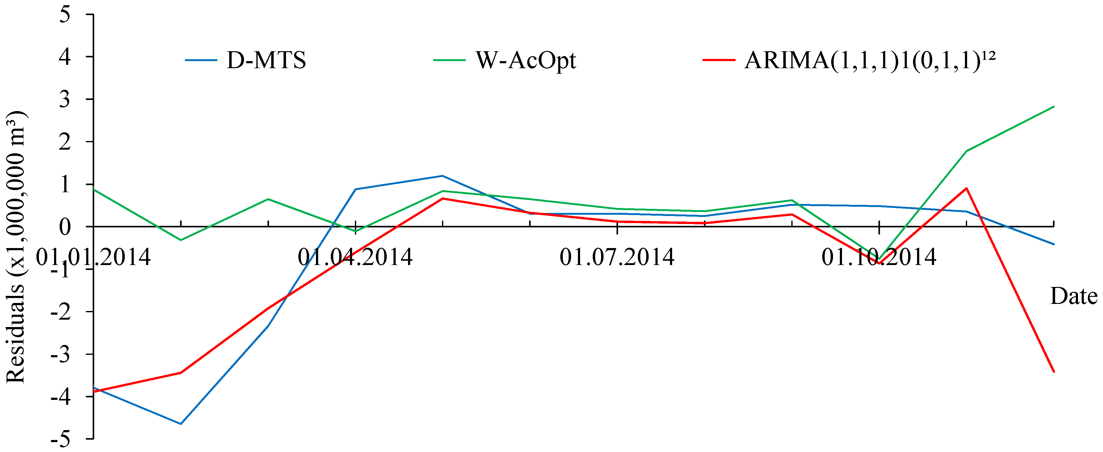
Figure 6 presents the 2014 residual graph of the lowest MAPE
2014 values observed using the three estimation methods. The time series decomposition is represented in blue, Holt-Winters is represented in green and SARIMA is represented in red in the series. The fact that winter consumption is 10 times greater than summer consumption, is also seen in the estimation errors. Although residuals are low during the summer period, in winter 5 times more residuals occur than in summer.
The methods studied in this paper are currently used on research related to the energy sector, mainly, in wind speed, hot water demand and wind power generation. For instance, Prema and Rao applied Holt-Winters, ARIMA and time series decomposition methods, and they found 28.63%, 23.26%, 18.24% MAPE’, respectively. They also mentioned that 30% MAPE is acceptable by the Government of India [
37]. We found MAPE for the time series decomposition, Holt-Winters and ARIMA methods at 19%, 14% and 12.9% respectively. Gelažanskas and Gamage found the R value for the time series decomposition, Holt-Winters and ARIMA to be 0.863, 0.811, 0.872 respectively [
36] to forecast hot water demand. In our study, the Ṙ² value of the time series decomposition, Holt-Winters and ARIMA are 0.915, 0.846 and 0.956, respectively. Wu and Peng introduced a wind power generation forecasting model and they compared their result with the ARIMA method [
60]. They found 38.57% MAPE with ARIMA forecasting whereas we achieved a three times lower MAPE. Our results prove that these methods are suitable for the natural gas demand forecast over the mid-term range, over a year measured on a monthly basis.
8. Conclusions
The main reasons for households and low consuming commercial users to use natural gas are heating, cooking and water heating. Even though cooking and water heating routinely occur, heating only appears in the winter period. Natural gas consumption also increases related to infrastructure investments and growth. The data used for forecasting in this study is prepared for the Sakarya province of Turkey. Households and low consuming commercial users’ 4-year consumption data between years 2011–2014 are gathered in monthly periods. This consumption data decreases in the summer while it increases in the winter. Therefore, the study researches natural gas demand forecasting by applying univariate seasonal and statistical methods. Well-known techniques of Time Series Decomposition and Winters Exponential Smoothing can be easily applied with spreadsheet software in daily life. However, ARIMA models need moderate knowledge and software containing ARIMA methods. Decision makers can use the natural gas demand forecasting results obtained from forecasting models as decision support systems. Therefore, they can comfortably use the supporting system for determining year-ahead demand and show the consistency of forecasts by comparing their prediction and statistical method results.
Based on the results, the main conclusions of the paper are as follows: the stationary of the series cannot be accepted after applying one time differencing because the series still include seasonality. Taking advantage of applying various methods such as time series decomposition, Holt-Winters exponential smoothing, and ARIMA-SARIMA, it is evaluated that the error rates decrease as the computation complexity of the method increases. Also the fact that infrastructure investments of the region where the data is gathered are almost completed, the investigated dataset does not show an increasing trend in consumption. However, the time series decomposition method, such as the simplest method, can be used by decision makers by calculating one by one, manually without using any statistical software. Moreover, even the worst case in the D-AS model is 0.907 Ṙ², 20% MAPE, 15% MAPE
2014 which is a better result than [
36,
37]. This outcome shows the possibility of forecasting natural gas demand.
Future research of this study will be in three different directions. The first case will use independent variables such as temperature, humidity, wind speed, number of subscribe and unit price if applicable. The second case applies methods such as ARIMAX (ARIMA with exogenous), regression models, learning algorithms, etc. The last case involves changing the time density such as using daily forecasts to make monthly estimations for a year.


