Abstract
The future uptake of electric vehicles (EV) in low-voltage distribution networks can cause increased voltage violations and thermal overloading of network assets, especially in networks with limited headroom at times of high or peak demand. To address this problem, this paper proposes a distributed battery energy storage solution, controlled using an additive increase multiplicative decrease (AIMD) algorithm. The improved algorithm (AIMD+) uses local bus voltage measurements and a reference voltage threshold to determine the additive increase parameter and to control the charging, as well as discharging rate of the battery. The used voltage threshold is dependent on the network topology and is calculated using power flow analysis tools, with peak demand equally allocated amongst all loads. Simulations were performed on the IEEE LV European Test feeder and a number of real U.K. suburban power distribution network models, together with European demand data and a realistic electric vehicle charging model. The performance of the standard AIMD algorithm with a fixed voltage threshold and the proposed AIMD+ algorithm with the reference voltage profile are compared. Results show that, compared to the standard AIMD case, the proposed AIMD+ algorithm further improves the network’s voltage profiles, reduces thermal overload occurrences and ensures a more equal battery utilisation.
1. Introduction
The adoption of electric vehicles (EV) is seen as a potential solution to the decarbonisation of future transport networks, offsetting emissions from conventional internal combustion engine vehicles. The current rate of EV uptake is anticipated to increase with improved driving range, reduced cost of purchase and greater emphasis on leading an environmentally-friendly lifestyle [1]. It is predicted that by 2030, there will be three million plug-in hybrid electric vehicles (PHEV) and EVs sold in Great Britain and Northern Ireland [2], and it is expected that by 2020, every tenth car in the United Kingdom will be electrically powered [3]. It is anticipated that the majority of PHEV/EV will be charged at home, putting additional stress on the existing local low voltage distribution network, which must then cater for the increased demand in energy [4,5]. Uncontrolled charging of multiple PHEV/EV can raise the daily peak power demand, which leads to: increased transmission line losses, higher voltage drops, equipment overload, damage and failure [6,7,8,9]. Accommodating the increased demand and mitigation of such failures is a major area of research interest, with the focus mainly placed on the coordinating and support of home charging.
Demand Side Management (DSM) strategies for Distributed Energy Resources (DER), aim to alleviate the impacts of PHEV/EV home-charging and are a favoured solution. Mohsenian-Rad et al. in [10] developed a distributed DSM algorithm that implicitly controls the operation of loads, based on game theory and the network operator’s ability to dynamically adjust energy prices. Focusing on financial incentive-driven DSM strategies, in [11], a Time-Of-Use (TOU) tariff and real-time load management strategy was proposed, where disruptive charging is avoided by allocating higher prices to times of peak demand. Financial incentives have also become a drive towards optimising the operation of Battery Energy Storage Solutions (BESS) and Distributed Generation (DG) when including PHEV/EV into the problem formulation [12].
Research focused on grid support has been driven by the need to deliver long-term savings and to avoid the immediate costs and disruption of network reinforcements and upgrades. This area of research proposes the implementation of alternative solutions to support the adoption of low carbon technologies, such as EVs, heat pumps and the electrification of consumer products. To reduce the resulting increased peak demand, Mohsenian-Rad et al. developed an approach of direct interaction between grid and consumer to achieve valley-filling, by means of dynamic game theory [10]. In [13], a Multi-Agent System (MAS) was used to manage flexible loads for the minimisation of cost in a dynamic game. The use of aggregators has been proposed to allow the participation of a number of small providers to participate in network support, such as grid frequency response [14,15,16]. Yet without the availability of power demand forecasts, real-time control needs to be implemented.
Real-time DSM can either be implemented in a centralised or distributed control approach. In the former, a central controller relays control signals to its aggregated DERs, whereas the latter allows each DER to control itself. A common form of controlling DERs in this mode of operation is set-point control [17]. Using set-point control on multiple identically-configured DERs would yield optimal operation conditions if each DER’s control parameters (e.g., bus voltage) were shared. In a system without sharing network information, DER control algorithms have to be improved to prevent, for example, devices located furthest from the substation from being used more frequently than others.
This paper therefore presents an individualised BESS control algorithm that lets distributed batteries respond to fluctuations in real-time local bus voltage readings. The proposed algorithm is based on the robust Additive Increase Multiplicative Decrease (AIMD) type algorithm, yet implements a set-point adjustment based on the location of the controlled BESS. It will be shown how these home-connected batteries can mitigate the impact of additional loads (i.e., EV uptake), whilst assuring that all BESS are cycled equally.
The key contribution of this work can be summarised as a novel distributed battery storage algorithm for mitigating the negative impact of dynamic load uptake on the low-voltage network. This algorithm uses an individualised set-point control to regulate bi-directional battery power flow and, for convergence, extends the traditional AIMD algorithm. As a result, the developed battery control method reduces voltage deviation, over-currents and the inequality of battery usage. Reducing this usage inequality leads to a homogeneous usage of all of the distributed batteries and, hence, prevents unequal degradation rates and unfair device utilisation.
The remainder of this paper is organised as follows: Section 2 gives some background to related work on AIMD algorithms on which this research is based. Section 3 outlines the EV, network and storage models used in the research. Additionally, it explains the assumptions that accommodate and justify these models. Section 4 elaborates on the proposed AIMD control algorithm (AIMD+). Next, Section 5 details the implementation and scenarios used for a set of test cases. For later comparison, this section also outlines a set of comparison metrics. Section 6 presents and discusses the results, followed by the conclusion in Section 7.
2. Related Work
Existing literature addresses the usage of energy storage units in low-voltage distribution networks to assure voltage security [18,19,20,21,22]. An approach used by, e.g., Mokhtari et al. in [21] relies on bus voltage and network load measurements to prevent system overloads. Yet, these kinds of storage control systems do require communication infrastructures to relay the network information and control instructions. This requirement has also been addressed in the comprehensive review on storage allocation and application methods by Hatziargyriou et al. [23]. In the presented work, a control algorithm is proposed that removes the need for such an inter-BESS communication, since it only uses local voltage measurements to infer the network operation. Yet, to prevent conflicting device behaviour, the underlying coordination mechanism is of particular importance. Assuring convergence, the AIMD algorithm is perfectly suited for such coordinated control.
Originally, AIMD algorithms were applied to congestion management in communications networks using the TCP protocol [24], to maximise utilisation while ensuring a fair allocation of data throughput amongst a number of competing users [25]. AIMD-type algorithms have previously been applied to power sharing scenarios in low voltage distribution networks, where the limited resource is the availability of power from the substation’s transformer.
For instance, such an algorithm was first proposed for EV charging by Stüdli et al. [26], requiring a one-way communications infrastructure to broadcast a “capacity event” [27,28]. Later, their work was further developed to include vehicle-to-grid applications with reactive power support [29]. The battery control algorithm proposed in this paper builds upon the algorithm used by Mareels et al. [30], where EV charging was organised by including bidirectional power flow and the use of a reference voltage profile derived from network models. Similar to the work by Xia et al. [31], who utilised local voltage measurements to adjust the charging rate, only voltage measurements at the batteries’ connection sites were used in this work to control the batteries’ operations.
Previous research is therefore extended by the work presented here, as previous work has only utilised common set-point thresholds for controlling each of the DERs. The approach proposed in this paper ensures that unavoidable voltage drops along the feeder do not skew the control decisions, and voltage oscillations caused by demand variation are taken into control considerations. In contrast to previous work, where substation monitoring was used to inform control units of the transformer’s present operational capacity, the proposed AIMD+ algorithm does not require this information and, hence, does not require such an extensive communications infrastructure.
3. System Modelling
In this section, the underlying assumptions to validate the research are addressed. Next, a model to describe EV charging behaviour is explained. This is followed by a model of the BESS. Finally, the network models used to simulate the power distribution networks are explained.
3.1. Assumptions
For this work, several underlying assumption were made to obtain the models:
- The uptake of EVs is assumed to increase and, hence, to have a significant impact on the normal operation of the low voltage distribution network. This assumption is based on a well-established prediction that the majority of EV charging will take place at home [32].
- The transition from internal combustion engine-powered vehicles to EVs is assumed to not impact the users’ driving behaviour. Similar to [33], this assumption allows the utilisation of recent vehicle mobility data [34] to generate leaving, driving and arriving probabilities, from which the EV charging demand can be determined.
- The transition to low carbon technologies will increase the variability of electricity demand, and therefore, grid-supporting devices, such as BESS, are anticipated to play a more important role [35]. Hence, alongside a high uptake of EVs, an increased adoption of distributed BESS devices is assumed.
- It is assumed that BESS solutions, or more specifically battery energy storage solutions, start the simulations at 50% SOC and are not 100% efficient at storing and releasing electrical energy, as in [36]. Additionally, its utilisation will degrade the energy storage capability and performance over time, as shown in [37]. Therefore, the requirements for equal and fair storage usage is of high importance.
- It is assumed that the load profiles provided by the IEEE Power and Energy Society (PES) are sufficient as base load profiles for all simulations.
3.2. Electric Vehicle Charging Behaviour
From publicly-available car mobility data [33,34] an empirical model was developed to capture the underlying driving behaviour. The raw data, , represents the probabilities of starting a trip during a 15-min period of a weekday. Three continuous normal distribution functions, each defined as:
were used to represent vehicles leaving in the morning, , lunch time, , and in the evening, . The aggregate probability of these three functions was optimised using a Generalised Reduced Gradient (GRG) algorithm to fit the original data. In order to represent a symmetric commuting behaviour, i.e., vehicles departing in the morning and returning during the evening, an equality amongst the three probabilities was defined as follows:
The resulting parameters from the GRG fitting of the three distribution functions are tabulated in Table 1. Additionally, the resulting departure probabilities, as well as the reference data are shown in Figure 1.

Table 1.
Parameters for normal distributions.
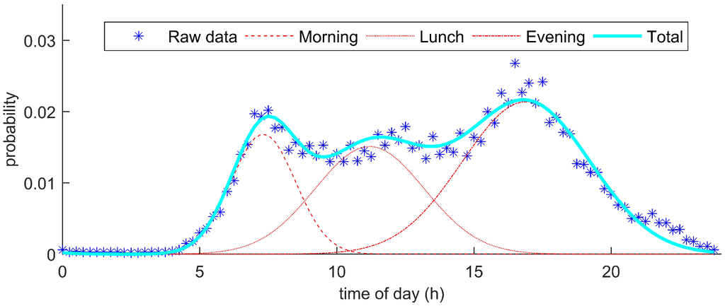
Figure 1.
The probability of starting a trip at a particular time during a weekday, extrapolated into three normal distributions (RMS error: ).
Statistical data capturing the probability distribution of a trip being of a certain distance were also extracted from the dataset. This was done for both the weekdays and weekends . The Weibull function was chosen to be fitted against the extracted probability distributions and is defined as:
Performing the curve fitting using the GRG optimisation algorithm, a weekday trip distance distribution, , and a weekend trip distribution, , could be estimated. The computed function parameters for these two estimated distribution functions are tabulated in Table 2. Their resulting probability distributions are plotted for comparison against the real data, and , in Figure 2.
Table 2.
Parameters for Weibull distributions.
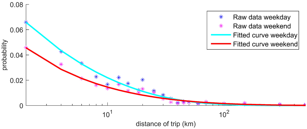
Figure 2.
The probability of a trip being of a particular distance during a weekday, extrapolated into a Weibull distribution (RMS error: ).
In addition to these probabilities, an average driving speed of 56 kmh (35 mph) and an average driving energy efficiency of 0.1305 kWh/kmh (0.21 kWh/mph) are taken from [38]. Using the predicted driving distance and average driving speed with the driving energy efficiency, it is possible to estimate an EV’s energy demand upon arrival. Starting to charge from this arrival time until the energy demand has been met allows the generation of an estimated charging profile of a single EV. To do this, a maximum charging power of the U.K.’s average household circuit rating (i.e., 7.4 kW) and an immediate disconnection of the EV upon charge completion were assumed [39].
Generating several of those charging profiles and aggregating them produces an estimated charging demand for an entire fleet of EVs. To provide an example, charge demand profiles for 50 EVs were generated, aggregated and plotted in Figure 3. This plot shows the expected magnitude and variability in energy demand that is required to charge several EVs at consumers’ homes based on the vehicles’ daily usage.
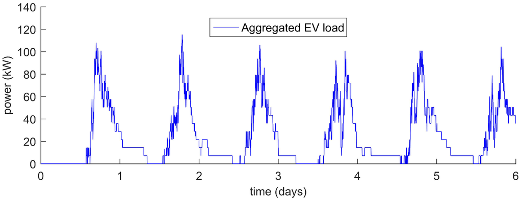
Figure 3.
Excerpt from the aggregated 50 EVs; charging powers that were each generated from the empirical models.
This model’s EV charging behaviour has been implemented to reflect EV demand if applied today without widespread smart charging infrastructure. It does therefore reflect the worst case scenario. Future smart-charging schemes would mitigate the currently present collective EV charging spike, yet the implementation and validation of available smart-charging schemes lies beyond the scope of this paper. This model’s data were used to feed additional demand into the power network models, which are outlined in the next section.
3.3. Battery Modelling
For this work, a well-established model that has been used in previous publications by this research group was used [36,40,41]. This model consists of a battery with a self-discharge loss that is dependent on the current battery’s State Of Charge (SOC) and an energy conversion loss to represent the energy lost when charging or discharging this battery. A complete list of all notations that are used for this battery model is included in Table 3.
Table 3.
Table of the notation used in this section.
When an ideal battery charges or discharges, the change in SOC is related by the battery power, . When sampling battery operation at a regular period, τ, then the energy transferred into the battery can be described as . The change in SOC for this ideal battery, , is therefore defined as:
The self-discharge loss is added to this ideal battery model to represent the continual loss of energy in the battery typical of chemical energy storage. This self-discharge loss, , is proportional to the current SOC and is determined using the self-discharge loss factor, μ:
Additionally, to represent the losses in the power electronics and energy conversion process, an energy conversion loss, , is defined. This loss is proportional to the rate at which the battery’s SOC changes, by using the energy conversion efficiency, as follows:
Here, the conversion losses in the power electronics are reflected as an asymmetric efficiency, which depends on the direction of the flow of energy. This is done by charging the battery at a lower power when consuming energy and discharging it more quickly when releasing energy. Mathematically, this can be represented as:
When substituting the self-discharge loss and conversion losses, respectively and , into the SOC evolution equation, the full battery model can be summarised as follows:
3.4. Network Models
To simulate the low-voltage energy distribution networks, the Open Distribution System Simulator (OpenDSS) developed by the Electronic Power Research Institute (EPRI) was used. It requires element-based network models, including line, load and transformer information, and generates realistic power flow results.
Simulations were conducted using the IEEE’s European Low Voltage Test Feeder [42] and six detailed U.K. feeder models, that are based on real power distribution networks and provided by Scottish and Southern Energy Power Distribution (SSE-PD). The SSE-PD circuit models were provided as Common Information Models (CIM) during the collaboration on the New Thames Valley Vision Project Project (NTVV) [43]. An example of the IEEE EU LV Test feeder and a U.K. feeder provided by SSE-PD are shown in Figure 4a,b, respectively. A summary of these model’s parameters is given in the Table 4.
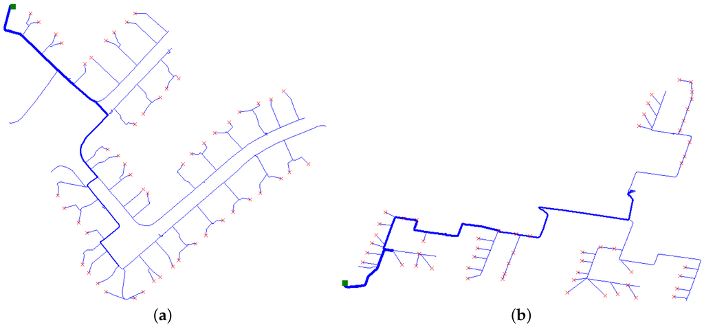
Figure 4.
Sample Open Distribution System Simulator (OpenDSS) power flow plots of the used power networks. Consumers are indicated as red crosses and 11/0.416-kV substations are marked with a green square. (a) IEEE Power and Energy Society (PES) EU Low Voltage Test Feeder plot; (b) Scottish and Southern Energy Power Distribution (SSE-PD) Common Information Model (CIM) (UK) feeder plot.
Table 4.
Network model parameters.
Throughout this paper, all excerpt and time series results were extracted from experiments with the IEEE EU LV Test feeder (i.e., Network No. 1). All concluding results are based on an aggregation of all networks to include network diversity in the analysis.
The model-derived EV data and IEEE EU LV Test feeder consumer demand profiles were used in all simulations. The resultant demand profiles represent the total daily electricity demand of households with EVs. These profiles were sampled at . The OpenDSS simulation environment was controlled using MATLAB, achieved through OpenDSS’s Common Object Model (COM) interface and accessible using Microsoft’s ActiveX server bridge.
4. Storage Control
In this section, the control of the energy storage system is explained. Firstly, the additive increase multiplicative decrease algorithm is presented, and its decision mechanism is explained in full. Then, the voltage referencing, used for AIMD+, is outlined.
4.1. Additive Increase Multiplicative Decrease
The proposed distributed battery storage control is shown in Algorithm 1. The parameter α denotes the size of the power’s additive increase step, and β denotes the size of the multiplicative decrease step. It is worth mentioning that α linearly increases and β exponentially decreases, both charging and discharging powers, where discharging power is represented as a negative power flow, i.e., energy released by the battery. The constants and are the maximum historic voltage value and the set-point threshold used to regulate the total demand. In the case when the total demand is too high, the local voltages will fall below , and the batteries reduce their charging power and start discharging. This behaviour reduces total demand on the feeder. At simulation start, is set to the nominal voltage of the substation transformer, i.e., 240 V, and is set to a fraction of , which was found by solving a balanced power flow analysis. The variable is the battery’s local bus voltage, and denotes the maximum charging/discharging power of the battery. The charging and discharging power of the batteries is increased in proportion to the available headroom on the network, which is inferred from the local voltage measurement , to avoid any sudden overloading of the substation transformer.
| Algorithm 1 Compute battery power. | ||
| 1: | ▷ Defines the rate for the current voltage reading | |
| 2: | if then | ▷ Given the voltage levels are nominal... |
| 3: | if then | ▷ ...and the battery is not fully charged... |
| 4: | ▷ ...increase the charging power | |
| 5: | else | ▷ If the battery has fully charged... |
| 6: | ▷ ...shut off | |
| 7: | end if | |
| 8: | if then | ▷ If the battery has been discharging... |
| 9: | ▷ ...reduce the discharging power by β | |
| 10: | end if | |
| 11: | else | ▷ If voltage levels are not nominal... |
| 12: | if then | ▷ ...and battery is charged sufficiently... |
| 13: | ▷ ...increase discharge power | |
| 14: | else | ▷ If the battery is not sufficiently charged... |
| 15: | ▷ ...shut off | |
| 16: | end if | |
| 17: | if then | ▷ If the battery has been charging... |
| 18: | ▷ ...reduce the charging power by β | |
| 19: | end if | |
| 20: | end if | |
| 21: | ▷ Limit the power to battery specifications | |
The algorithm itself, as shown in Algorithm 1, contains two decision levels. The first determines whether the network is over- or under-loaded by comparing the local bus voltage, , to the battery’s set-point threshold, . In the event that the network is not under high load, the battery’s SOC is compared to its operation limit to check whether the battery can charge, i.e., < . If there is enough charging capacity left, then the battery’s charging power is linearly increased following Line 4. If the battery was previously discharging, the related discharging power is exponentially reduced (Line 9) to reflect the multiplicative decrease.
The second decision level is entered when the network is under load. Here, the discharging power is linearly increased if the battery has enough energy stored, i.e., > (Line 13). Additionally, if the battery was previously charging, then its charging power is multiplicatively reduced (Line 18). The direction of the charging/discharging power adjustment is determined by the first decision level, as well as the threshold proximity ratio . As the battery’s bus voltage, , approaches the threshold voltage, , this ratio tends to zero and, hence, stops the battery operation. Therefore, oscillatory hunting is effectively mitigated. The last step of the algorithm (Line 21) assures that the battery charge/discharge power is within its device rating.
4.2. Reference Voltage Profile
When using a fixed voltage threshold, the difference in the location and load of each customer results in the over-utilisation of batteries located at the feeder end. Similar to Papaioannou et al. [44], yet for the control of BESS instead of EV charging, a reference voltage profile is proposed, which is produced by performing a power flow analysis of the network under maximum demand. An example of a fixed threshold and reference voltage profile is shown in Figure 5.
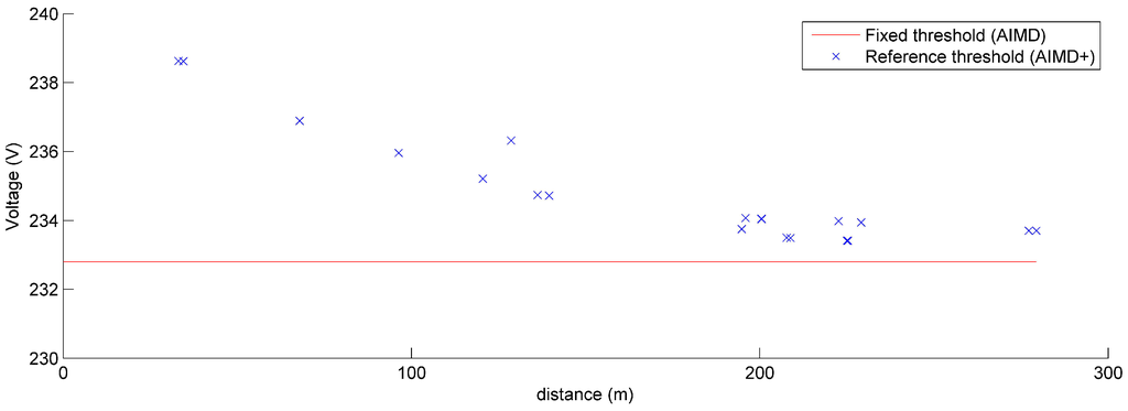
Figure 5.
A plot showing the difference between the fixed voltage threshold (AIMD) and the reference voltage profile (AIMD+).
In the AIMD+, consumers located at the head of the feeder are allocated a higher voltage threshold, while those towards the end of the feeder have similar voltage thresholds to that of the fixed threshold. This replicates the expected voltage drop along the length of the feeder, hence resulting in a more equal utilisation of battery storage units that are located at those distances. The voltage threshold is set in such a way as to limit the maximum voltage drop to 3% at the end of the feeder.
5. Scenarios and Comparison Metrics
In this section, several scenarios are explained that were used to test the performance of the battery control algorithm. Following that is the definition of three comparison metrics. These metrics quantify the improvements caused by the different algorithms in comparison to the worst case scenario.
5.1. Test Cases and Scenarios
In all simulations, the EVs plug-in on arrival and charge at their nominal charging rate until fully charged. The BESS devices were chosen to have a capacity of 7 kWh with a maximum power rating of 2 kW (battery specifications are based on the Tesla Powerwall [45]). Four excerpt cases were defined with different levels of EV and storage uptakes, these are as follows:
- A
- A baseline scenario, where only household demand is used.
- B
- A worst case scenario, in which EV uptake is 100% and no BESS is used.
- C
- An AIMD scenario, in which EV uptake is 100% and each household has a battery energy storage device. Here, each battery was controlled using the AIMD algorithm using a fixed voltage threshold.
- D
- An AIMD+ scenario, in which EV uptake is 100%, and each household has a battery energy storage device. Here, each battery was controlled using the AIMD+ algorithm using the optimised reference voltage profile.
A storage uptake of 100% was adopted to represent the worst case scenario. In addition to the four defined scenarios, a full set of simulations was performed with EV and storage uptake combinations of 0% to 100% in steps of 10%.
5.2. Performance Metric Definition
To obtain comparable performance metrics, three parameters are defined. These parameters capture the improvements in voltage violation mitigation, line overload reduction and the equality of battery usage. All excerpt performance metrics were calculated based on simulations from the IEEE EU LV Test feeder for reproducibility.
5.2.1. Parameter for Voltage Improvement
The first parameters are and for, respectively, Cases C and D, and calculate the magnitude of the voltage level improvement by comparing two voltage frequency distributions. More specifically, they find the difference between these probability distributions and compute a weighted sum. Here, the weighting, , emphasises the voltage level improvements that deviate further from the nominal substation voltage . If the resulting weighted sum is negative, then the obtained voltage frequency distribution was improved in comparison to the associated worst case scenario. In contrast, a positive number would indicate a worse outcome. The performance metric is defined as follows.
Here, is the lowest recorded voltage, and is the highest recorded voltage. is the voltage probability distribution of the worst case scenario (Case B), and is the voltage probability distributions of Case C (i.e., the case with maximum EV and AIMD storage uptake). Similarly, the parameter therefore compares Case D, i.e., the AIMD+ case, with Case B.
The aforementioned factor, , scales down the summation in Equation (11) for voltages within the nominal operating band, where no voltage violations take place. Voltage violations on the other hand are scaled up to increase their impact on the summation. This scaling was produced using a linear function, with its minimum at , that is defined as:
and are defined as the lower and upper limits of the nominal operation voltage band, respectively. In general, the proposed voltage comparison parameter, , shows an improvement in voltage distribution when it is negative, whereas a positive value implies a voltage distribution with more voltage violations.
5.2.2. Parameter for Line Overload Reduction
Similar to measuring the voltage level improvements, all line utilisation probability distributions between the storage and worst case scenarios were compared. This follows a similar equation to before, but uses a different scaling factor, as described in Equation (11):
Here, is the highest line utilisation. and present the line utilisation probability distributions for Cases B and C, respectively, and is the associated scaling factor. Since the relationship between line current and ohmic losses is quadratic, this scaling factor is defined as an exponential function that amplifies the impact of line currents beyond the line’s nominal rating.
The capacity scale modifier, , defines from where the scaling should start and has been set to for this work as only line utilisation above p.u. was considered. Therefore, a reduction in line overloads would give a negative , whereas a positive value implies a higher line utilisation, i.e., worse results.
5.2.3. Parameter for the Improvement of Battery Cycling
The final metric, , gives an indication of the inequality of battery cycling (one battery cycle is defined as a full discharge and charge of the battery at maximum operating power, i.e., ) across all battery units. It does this by computing the the ratio between the peak and mean battery cycling. This Peak-to-Average Ratio (PAR) of batteries’ cycling is defined in the following equation.
Here, B is the number of batteries, and is the total cycling of battery b during Scenario C. is a vector of that contains all batteries’ cycling values, i.e., . Equally, the battery cycling for Scenario D would be captured by . In the unlikely event of an equal cycling of all batteries, will have a value of one. Yet, as batteries are operated differently, the value of is likely to be greater than one. Therefore, a resulting PAR closer to one implies a more equal and therefore fairer utilisation of the deployed batteries.
6. Results and Discussion
In this section, the results are outlined that were generated from all simulations. In each of the three subsections, the performances of the AIMD and AIMD+ algorithm are compared against each other. To do so, the performance metrics outlined in Section 5.2 were used. In the following subsections, results from the four test cases defined as A, B, C and D in Section 5.1 are explained first, then the results from the full analysis over the large range of EV and battery storage uptake is presented. In the end, these results are summarised and discussed.
6.1. Voltage Violation Analysis
For the comparison of voltage improvements, results compared the algorithms’ performances at reducing bus voltage variation; particularly by increasing the lowest recorded bus voltage. Each load’s bus voltage was recorded, from which a sample voltage profile, Figure 6, was extracted, where the bus voltage fluctuation over time becomes apparent. It can be seen that the introduction of EVs has significantly lowered the line-to-neutral voltage. Adding energy BESS devices did raise the voltage levels during times of peak demand, as can be seen between 17:00 and 21:00, where the AIMD+ algorithm has elevated voltages further than the AIMD scenario. To obtain a better understanding of the level of improvement, the voltage frequency distribution of all buses along the feeder was generated and plotted in a histogram in Figure 7.
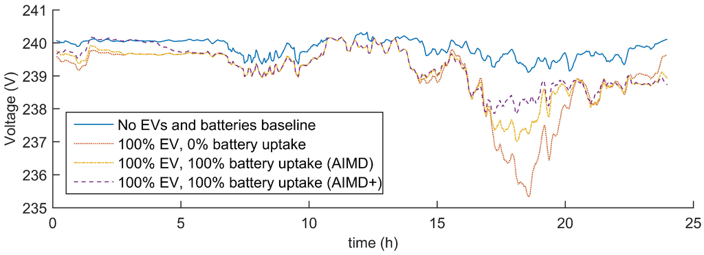
Figure 6.
Recorded voltage profile at the bus of the customer closest to the substation over the period of one day with a certain uptake in EV and battery storage devices using a moving average over a window of 5 min. Here, Case A is blue; Case B is red; Case C is yellow; and Case D is violet.
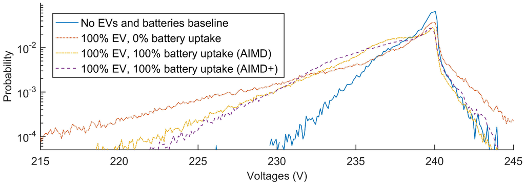
Figure 7.
Voltage probability distribution of all loads’ buses for certain uptakes of EV and battery storage devices. Here, Case A is blue; Case B is red; Case C is yellow; and Case D is violet; with and .
In this histogram, the voltage probability distributions for all four cases were normalised and plotted against each other. Here, the previously seen drop in voltages by introducing EVs is recorded as a shift in the voltage distribution. This voltage drop is mitigated by the introduction of the storage solutions, since the probability distribution is shifted towards higher voltage bands. For the IEEE EU LV Test feeder, the AIMD+-controlled batteries outperform the AIMD devices as the resulting is greater than .
To gain a full understanding of the performance of the AIMD and AIMD+ algorithms, a full sweep of EV and BESS uptake combinations was simulated on all available power distribution networks. The resulting parameters were averaged and plotted in Figure 8.
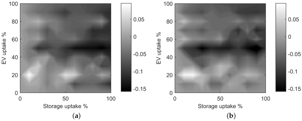
Figure 8.
Comparison of voltage improvement indices (i.e., ) for (a) AIMD and (b) AIMD+. (a) indices (AIMD); (b) indices (AIMD+).
These figures show that the AIMD+ control algorithm reduces voltage deviation more effectively as the uptake in storage and EVs increases. For low storage uptake, the AIMD algorithm does not perform as strongly since more values are positive and larger than their corresponding value. This becomes more apparent when averaging all and values for their common storage uptake and across all EV uptakes. The resulting averaged metrics are plotted in Figure 9.
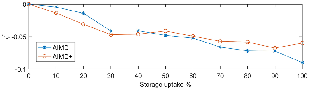
Figure 9.
Average (AIMD) and (AIMD+) values recorded against the corresponding storage uptake.
In this last figure, it can be seen how the sole impact of BESS uptake reflects in a continuing improvement of voltage levels. In fact, both compared algorithms improved the bus voltage, which coincides with the findings in the case studies. On average, this is the case for all BESS uptakes, as . Nonetheless, it should be noted that the AIMD+ algorithm had reduced the frequency of severe voltage deviations in comparison to the AIMD algorithm and is more effective during scenarios with lower BESS uptake.
6.2. Line Overload Analysis
Similar to the voltage improvement analysis, a frequency distribution of the line utilisation was generated. Figure 10 shows a probability distribution of the per unit (1 p.u. represents a 100% line usage, i.e., a line current of the same value as the line’s nominal current rating) current in all lines, for each of the four scenarios. The corresponding and values for the AIMD and AIMD+ storage deployment have also been included in the figure’s caption. In this figure, the observed high probability of line over-utilisation confirms that the used test network is of insufficient capacity to cater for the chosen EV uptake.
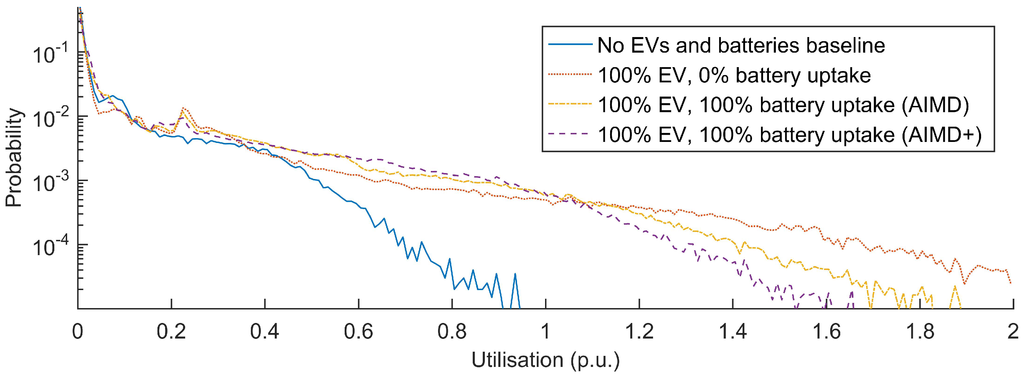
Figure 10.
Line utilisation probability distribution of all lines in the simulated feeder for certain uptakes of EV and battery storage devices. Here, Case A is blue; Case B is red; Case C is yellow; and Case D is violet; with and .
Here, the AIMD+ controlled storage devices yielded a noticeable reduction in line overloads. This improvement is apparent through the compressed width of the probability distribution and the negative value. In contrast, the AIMD controlled storage devices do not fully utilise the line capacity as effectively, which leads to a positive value of . To evaluate the line utilisation improvement across all simulations, the full range of EV and storage uptake was evaluated. The resulting plots are shown in Figure 11.
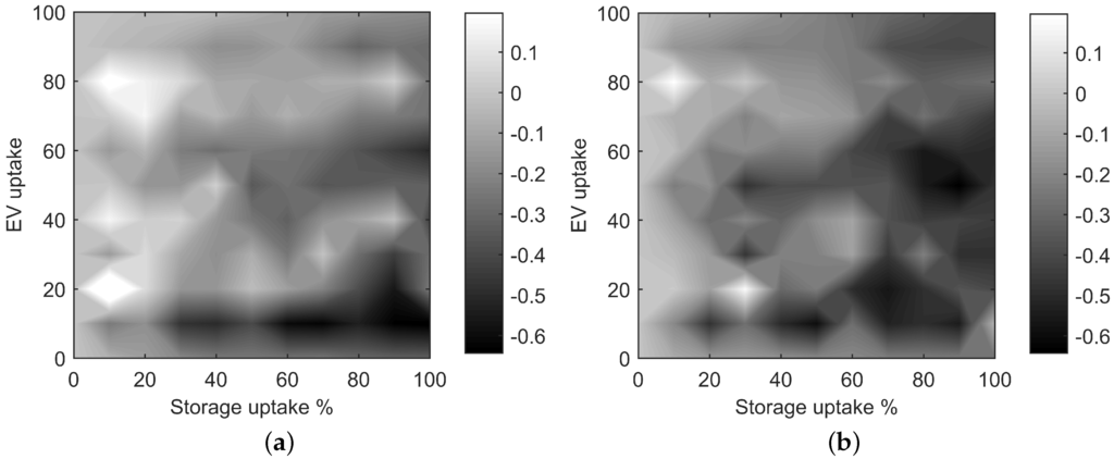
Figure 11.
Comparison of line utilisation improvement indices for (a) AIMD and (b) AIMD+. (a) indices (AIMD); (b) indices (AIMD+).
In these figures, it can be seen how the performance metrics change as EV uptake and storage uptake increase. For the AIMD-controlled BESS, the resulting values are distributed around zero, whereas the AIMD+ algorithm achieved mostly negative values of . These negative values confirm the better usage of available line capacity. This becomes particularly noticeable for scenarios where very low EV uptake is combined with larger BESS uptake. Here, AIMD-controlled storage devices commence their initial charge simultaneously. As they are located closer to the substation, they do not measure a sufficient bus voltage offset to regulate down their charging power. This behaviour causes a number of line overloads at the very beginning of the simulated days. The AIMD+ algorithm on the other hand, with its adjusted thresholds, is more responsive to non-optimal network operation and, therefore, increases the charging rate gradually.
This gradual adjustment is based on the fact that the bus voltages in the AIMD+ algorithm are closer to their nominal voltages (i.e., bus voltages found by simulating the feeder with its equally-distributed nominal load) than they are in the conventional AIMD case. A greater voltage disparity, which is the case in AIMD, causes a prolonged additive adjustment to the battery’s power. This prolonged adjustment is particularly apparent for batteries situated at the bottom of the feeder, as their voltage measurements deviate the furthest from the substation voltage level. AIMD+ on the other hand prevents this behaviour by setting the voltage threshold based on the network’s nominal voltage drop, which is dependent on the distance between the BESS and its feeding substation. As a result, the set-point voltage thresholds at the bottom of the feeder are lower than those closer to the substation. Hence, the additive power adjustment is equalised along the entire feeder. Therefore, by applying these individualised control thresholds, the sensitivity of the algorithm is corrected, whilst successfully mitigating the severity of line overloads.
Averaging the and values over all EV uptakes gives a clearer indication of performance, as this is now the only variable in the performance analysis. The result is plotted in Figure 12. Here, the hypothesis that AIMD-controlled energy storage devices do not improve line utilisation is confirmed. In contrast, the AIMD+-controlled devices succeed at effectively reducing line overloads. This is also demonstrated by the values of , which remain positive yet close to zero, whereas decreases with increasing uptake of battery storage devices.
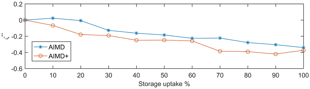
Figure 12.
Average (AIMD) and (AIMD+) values recorded against the corresponding storage uptake.
Whilst the deployment of energy storage has often been seen as a possible solution to defer network reinforcements, the presented results show that this is not always the case. In fact, the importance of choosing an appropriate control algorithm outweighs the availability of the energy storage itself. This becomes particularly apparent when energy storage devices need to recharge their injected energy for times of peak demand. For the AIMD case, this recharging was not controlled sufficiently, which led to higher line currents. The proposed AIMD+ algorithm was not as susceptible to this kind of behaviour, as it has been designed to take battery location into account. This immunity and well-controlled power flow caused little to no additional strain on the network’s equipment, allowing the deployed storage devices to also provide voltage support.
6.3. Battery Utilisation Analysis
In this part of the analysis, the batteries’ fairness of usage was evaluated. The battery power profiles were recorded; excerpts are plotted in Figure 13 and are arranged by distance from the substation.
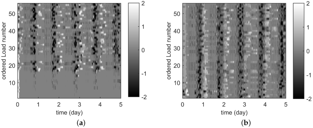
Figure 13.
Battery power profiles of each load’s battery storage device over four days for (a) AIMD and (b) AIMD+. (a) Case C, 60% EV and 100% AIMD (kW); (b) Case D, 60% EV and 100% AIMD+ (kW).
In this figure, it can be seen that only half of the deployed storage devices were active in Case C (AIMD control), whereas all devices are utilised in Case D (AIMD+ control). From the recorded battery SOC profiles, the net cycling of each battery was computed and divided by the duration of the simulation, giving an average daily cycling value. This value is plotted for each load in Figure 14a. The corresponding statistical analysis is presented in Figure 14b.
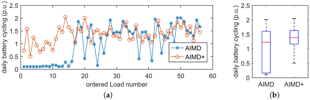
Figure 14.
Each load’s battery cycling compared for (a) 60% EV and 100% AIMD and AIMD+ uptake and (b) in a statistical context. Here, and . (a) Battery cycling for each load; (b) statistic.
These two plots show the under-usage of AIMD controlled batteries, as well as the variance in battery usage under AIMD and AIMD+ control. In fact, under AIMD control, 20 out of 55 batteries experienced a cycling of less than 10% per day, whereas the remaining devices were utilised fully. This discrepancy causes the value to be noticeably larger than . A more detailed comparison is given when plotting the Peak-to-Average Ratios (PAR) of the batteries’ daily cycling over the full range of EV and storage uptake scenarios; these plots are shown in Figure 15. Section 5.2.3 gives the detail on the PAR, .
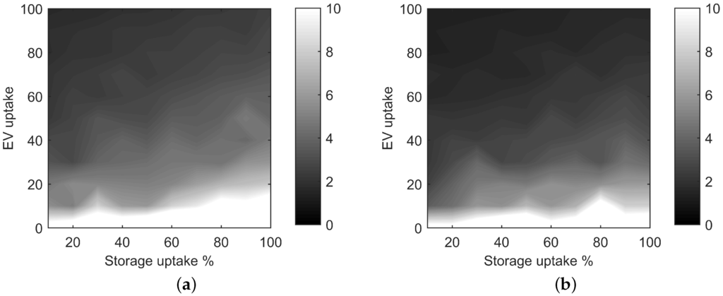
Figure 15.
Peak-to-Average Ratios (PAR) of the battery cycling profiles of each load’s battery storage device over four days for (a) AIMD and (b) AIMD+. (a) Cycling PAR for AIMD; (b) cycling PAR for AIMD+.
The figure shows that for any EV uptake scenario, AIMD-controlled energy storage units were cycled less equally than the AIMD+ controlled devices. Results also show that with a low EV uptake, both the AIMD and AIMD+ algorithm performed worse; yet improved as EV uptake increased.
Averaging the PARs for all batteries’ SOC profiles over all EV uptake percentages yields a clear performance difference between AIMD and AIMD+. These resulting PARs, i.e., the and values for their corresponding storage uptake percentages, are presented in Figure 16.
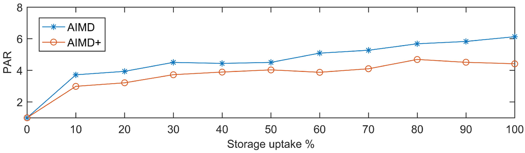
Figure 16.
The performance index for AIMD storage and for AIMD+ storage control against storage uptake.
Although the AIMD controlled batteries were, on average, cycled less than the batteries controlled by the proposed AIMD+ algorithm, looking at the average produces a distorted understanding of the performance. In fact, as more than half of the assigned AIMD BESS devices never partook in the network control, a lower average cycling was expected to begin with. The variation in cycling across all batteries, or the cycling PAR, reveals the difference between usage and effective usage. A lower ratio indicates a better usage of the deployed batteries.
7. Conclusions
In this paper, an algorithm is proposed for distributed battery energy storage, in order to mitigate the negative impact of highly variable uncontrolled loads, such as the charging of EVs. The improved AIMD algorithm uses local bus voltage measurements and implements a reference voltage profile, derived from power flow analysis of the distribution network, for its set-point control. Taking the distance to the feeding substation into account allowed optimising the algorithm’s parameters for each BESS. Simulations were performed on the IEEE EU LV Test feeder and a set of real U.K. suburban network models. Comparisons were made of the standard AIMD algorithm with a fixed voltage threshold against the proposed AIMD+ algorithm using a reference voltage threshold. A set of European demand profiles and a realistic EV travel model were used to feed load data into the simulations.
For all conducted simulations, the performance of the energy storage units was improved by using the proposed AIMD+ algorithm instead of traditional AIMD control. The improved algorithm resulted in a reduction of voltage variation and an increased utilisation of available line capacity, which also reduced the frequency of line overloads. Additionally, the same algorithm equalised the cycling and utilisation of battery energy storage, making better use of the deployed battery assets. To take this work further, future work will also consider distributed generation, such as photovoltaic panels, smart-charging EV uptake, as well as decentralised methods for determining voltage reference values, so no prior network knowledge is required.
Acknowledgments
The authors would like to thank SSE-PD for providing their network information for the utilised U.K. feeder models and also Miss Catriona Scrivener for proofreading this manuscript.
Author Contributions
Maximilian J. Zangs and Peter B. E. Adams contributed equally to this piece of work and were supervised by William Holderbaum and Ben A. Potter. Timur Yunusov has provided technical input and feedback throughout.
Conflicts of Interest
The authors declare no conflict of interest.
References
- Shah, V.; Booream-Phelps, J. F.I.T.T. for Investors: Crossing the Chasm; Technical Report; Deutsche Bank Market Research: Frankfurt am Main, Germany, 2015. [Google Scholar]
- Department for Business Enterprise and Regulatory (DBER); Department for Transport (DfT). Investigation into the Scope for the Transport Sector to Switch to Electric Vehicles and Plug-in Hybrid Vehicles; Technical Report; Department for Business Enterprise and Regulatory (DBER), Department for Transport (DfT): London, UK, 2008. [Google Scholar]
- Ecolane, University of Aberdeen. Pathways to High Penetration of Electric Vehicles; Technical Report; Ecolane, University of Aberdeen: Bristol, UK, 2013. [Google Scholar]
- Clement-Nyns, K.; Haesen, E.; Driesen, J. The impact of Charging plug-in hybrid electric vehicles on a residential distribution grid. IEEE Trans. Power Syst. 2010, 25, 371–380. [Google Scholar] [CrossRef]
- Fernández, L.P.; San Román, T.G.; Cossent, R.; Domingo, C.M.; Frías, P. Assessment of the impact of plug-in electric vehicles on distribution networks. IEEE Trans. Power Syst. 2011, 26, 206–213. [Google Scholar] [CrossRef]
- Hadley, S.W.; Tsvetkova, A.A. Potential Impacts of Plug-in Hybrid Electric Vehicles on Regional Power Generation. Electr. J. 2009, 22, 56–68. [Google Scholar] [CrossRef]
- Putrus, G.; Suwanapingkarl, P.; Johnston, D.; Bentley, E.; Narayana, M. Impact of electric vehicles on power distribution networks. In Proceedings of the IEEE Vehicle Power and Propulsion Conference, Dearborn, MI, USA, 7–10 September 2009; pp. 827–831.
- Pillai, J.R.; Bak-Jensen, B. Vehicle-to-grid systems for frequency regulation in an islanded Danish distribution network. In Proceedings of the IEEE Vehicle Power and Propulsion Conference (VPPC), Lille, France, 1–3 September 2010.
- Zhou, K.; Cai, L. Randomized PHEV Charging Under Distribution Grid Constraints. IEEE Trans. Smart Grid 2014, 5, 879–887. [Google Scholar] [CrossRef]
- Mohsenian-Rad, A.H.; Wong, V.W.S.; Jatskevich, J.; Schober, R.; Leon-Garcia, A. Autonomous demand-side management based on game-theoretic energy consumption scheduling for the future smart grid. IEEE Trans. Smart Grid 2010, 1, 320–331. [Google Scholar] [CrossRef]
- Deilami, S.; Masoum, A.S. Real-time coordination of plug-in electric vehicle charging in smart grids to minimize power losses and improve voltage profile. IEEE Trans. Smart Grid 2011, 2, 456–467. [Google Scholar] [CrossRef]
- Masoum, A.S.; Deilami, S.; Member, S.; Masoum, M.A.S. Fuzzy Approach for Online Coordination of Plug-In Electric Vehicle Charging in Smart Grid. IEEE Trans. Sustain. Energy 2015, 6, 1112–1121. [Google Scholar] [CrossRef]
- Karfopoulos, E.L.; Hatziargyriou, N.D. A Multi-Agent System for Controlled Charging of a Large Population of Electric Vehicles. IEEE Trans. Power Syst. 2013, 28, 1196–1204. [Google Scholar] [CrossRef]
- Wu, C.; Mohsenian-Rad, H.; Huang, J. Vehicle-to-aggregator interaction game. IEEE Trans. Smart Grid 2012, 3, 434–442. [Google Scholar] [CrossRef]
- Samadi, P.; Mohsenian-Rad, H.; Schober, R.; Wong, V.W.S. Advanced Demand Side Management for the Future Smart Grid Using Mechanism Design. IEEE Trans. Smart Grid 2012, 3, 1170–1180. [Google Scholar] [CrossRef]
- Xu, N.Z.; Chung, C.Y. Challenges in Future Competition of Electric Vehicle Charging Management and Solutions. IEEE Trans. Smart Grid 2015, 6, 1323–1331. [Google Scholar] [CrossRef]
- Leadbetter, J.; Swan, L. Battery storage system for residential electricity peak demand shaving. Energy Build. 2012, 55, 685–692. [Google Scholar] [CrossRef]
- Sugihara, H.; Yokoyama, K.; Saeki, O.; Tsuji, K.; Funaki, T. Economic and efficient voltage management using customer-owned energy storage systems in a distribution network with high penetration of photovoltaic systems. IEEE Trans. Power Syst. 2013, 28, 102–111. [Google Scholar] [CrossRef]
- Toledo, O.M.; Oliveira, D.; Diniz, A.; Martins, J.H.; Vale, M.H.M. Methodology for Evaluation of Grid-Tie Connection of Distributed Energy Resources-Case Study with Photovoltaic and Energy Storage. IEEE Trans. Power Syst. 2013, 28, 1132–1139. [Google Scholar] [CrossRef]
- Marra, F.; Yang, G.Y.; Fawzy, Y.T.; Træholt, C.; Larsen, E.; Garcia-Valle, R.; Jensen, M.M. Improvement of local voltage in feeders with photovoltaic using electric vehicles. IEEE Trans. Power Syst. 2013, 28, 3515–3516. [Google Scholar] [CrossRef]
- Mokhtari, G.; Nourbakhsh, G.; Ghosh, A. Smart coordination of energy storage units (ESUs) for voltage and loading management in distribution networks. IEEE Trans. Power Syst. 2013, 28, 4812–4820. [Google Scholar] [CrossRef]
- Atia, R.; Yamada, N. Sizing and Analysis of Renewable Energy and Battery Systems in Residential Microgrids. IEEE Trans. Smart Grid 2016, 7, 1204–1213. [Google Scholar] [CrossRef]
- Hatziargyriou, N.D.; Škrlec, D.; Capuder, T.; Georgilakis, P.S.; Zidar, M. Review of energy storage allocation in power distribution networks: Applications, methods and future research. IET Gener. Transmi. Distrib. 2015, 10, 1–8. [Google Scholar]
- Chiu, D.M.; Rain, R. Analysis of the increase and decrease algorithms for congestion avoidance in computer networks. Comput. Netw. ISDN Syst. 1989, 17, 1–14. [Google Scholar] [CrossRef]
- Wirth, F.; Stuedli, S.; Yu, J.Y.; Corless, M.; Shorten, R. IBM Research Report: Nonhomogeneous Place-Dependent Markov Chains, Unsynchronised AIMD, and Network Utility Maximization; Technical Report; IBM: New York, NY, USA, 2014. [Google Scholar]
- Stüdli, S.; Crisostomi, E.; Middleton, R.; Shorten, R. A flexible distributed framework for realising electric and plug-in hybrid vehicle charging policies. Int. J. Control 2012, 85, 1130–1145. [Google Scholar] [CrossRef]
- Studli, S.; Griggs, W.; Crisostomi, E.; Shorten, R. On Optimality Criteria for Reverse Charging of Electric Vehicles. IEEE Trans. Intell. Transp. Syst. 2014, 15, 451–456. [Google Scholar] [CrossRef]
- Stüdli, S.; Crisostomi, E.; Middleton, R.; Shorten, R. Optimal real-time distributed V2G and G2V management of electric vehicles. Int. J. Control 2014, 87, 1153–1162. [Google Scholar] [CrossRef]
- Stüdli, S.; Crisostomi, E.; Middleton, R.; Braslavsky, J.; Shorten, R. Distributed Load Management Using Additive Increase Multiplicative Decrease Based Techniques. In Plug in Electric Vehicles in Smart Grids; Springer: Singapore, Singapore, 2015; pp. 173–202. [Google Scholar]
- Mareels, I.; Alpcan, T.; Brazil, M.; de Hoog, J.; Thomas, D.A. A distributed electric vehicle charging management algorithm using only local measurements. In Proceedings of the IEEE PES Innovative Smart Grid Technologies Conference (ISGT), Washington, DC, USA, 19–22 February 2014; pp. 1–5.
- Xia, L.; Hoog, J.D.; Alpcan, T.; Brazil, M. Electric Vehicle Charging: A Noncooperative Game Using Local Measurements; The International Federation of Automatic Control: Cape Town, South Africa, 2014; pp. 5426–5431. [Google Scholar]
- Munkhammar, J.; Bishop, J.D.; Sarralde, J.J.; Tian, W.; Choudhary, R. Household electricity use, electric vehicle home-charging and distributed photovoltaic power production in the city of Westminster. Energy Build. 2015, 86, 439–448. [Google Scholar] [CrossRef]
- Dallinger, D.; Wietschel, M. Grid integration of intermittent renewable energy sources using price-responsive plug-in electric vehicles. Renew. Sustain. Energy Rev. 2012, 16, 3370–3382. [Google Scholar] [CrossRef]
- Institut für angewandte Sozialwissenschaft GmbH; Deutsches Zentrum für Luft-und Raumfahrt e.V. Mobilität in Deutschland 2008; Technical Report; Mobilität in Deutschland: Bonn und Berlin, Germany, 2008. [Google Scholar]
- National Grid. Future Energy Scenarios 2015; Technical Report; National Grid: Warwick, UK, July 2015. [Google Scholar]
- Rowe, M.; Member, S.; Yunusov, T.; Member, S.; Haben, S.; Singleton, C.; Holderbaum, W.; Potter, B. A Peak Reduction Scheduling Algorithm for Storage Devices on the Low Voltage Network. IEEE Trans. Smart Grid 2014, 5, 2115–2124. [Google Scholar] [CrossRef]
- Laresgoiti, I.; Käbitz, S.; Ecker, M.; Sauer, D.U. Modeling mechanical degradation in lithium ion batteries during cycling: Solid electrolyte interphase fracture. J. Power Sour. 2015, 300, 112–122. [Google Scholar] [CrossRef]
- Government Digital Service. Vehicle Free-Flow Speeds (SPE01); Government Digital Service: London, UK, 2013.
- Office for Low Emission Vehicles. Electric Vehicle Homecharging Scheme—Guidance for Manufacturers and Installers; Technical Report; Office for Low Emission Vehicles: London, UK, 2016. [Google Scholar]
- Rowe, M.; Holderbaum, W.; Potter, B. Control methodologies: Peak reduction algorithms for DNO owned storage devices on the Low Voltage network. In Proceedings of the 4th IEEE/PES Innovative Smart Grid Technologies Europe (ISGT), Lyngby, Denmark, 6–9 October 2013; pp. 1–5.
- Rowe, M.; Yunusov, T.; Haben, S.; Holderbaum, W.; Potter, B. The real-time optimisation of DNO owned storage devices on the LV network for peak reduction. Energies 2014, 7, 3537–3560. [Google Scholar] [CrossRef]
- Society, I.P. Energy, European Low Voltage Test Feeder. Available online: http://ewh.ieee.org/soc/pes/dsacom/testfeeders/ (accessed on 31 January 2016).
- Thames Valley Vision—Project Library—Published Documents. Available online: http://thamesvalleyvision.co.uk/project-library/published-documents/ (accessed on 31 January 2016).
- Papaioannou, I.T.; Purvins, A.; Demoulias, C.S. Reactive power consumption in photovoltaic inverters: A novel configuration for voltage regulation in low-voltage radial feeders with no need for central control. Prog. Photovolt. Res. Appl. 2015, 23, 611–619. [Google Scholar] [CrossRef]
- Tesla Motors Inc. Tesla Powerwall; Tesla Motors Inc.: Fremont, CA, USA, 2015. [Google Scholar]
© 2016 by the authors; licensee MDPI, Basel, Switzerland. This article is an open access article distributed under the terms and conditions of the Creative Commons Attribution (CC-BY) license (http://creativecommons.org/licenses/by/4.0/).