1. Introduction
More than half of the global population now resides in cities [
1]. As urban areas continue to sprawl, with the global urban population expected to increase by two to three billion this century, affluence-driven urbanization has been singled out as one of the key drivers of energy demand and climate change [
2,
3,
4]. In trying to respond to these trends, cities have become major players in assisting national governments in fast tracking transformative action for global climate change mitigation [
5,
6]. Cities even often lead the way in implementing mitigation strategies when there is lack of national abatement policies [
7,
8]. The Intergovernmental Panel on Climate Change (IPCC) has decided that a Special Report on Climate Change and Cities will be included in the Assessment Report Cycle [
9].
More than 400 mayors signed up to the Compact of Mayors, a global initiative to reduce emissions in cities through networking [
5]. 360 Compact of Mayors cities announced at the Paris Climate Conference in November 2015 that the collective impact of their commitments will deliver potential urban emissions reductions in 2030 equivalent to nearly 25% of the “gap” (15 GtCO
2e) between national pledges made in advance of the 2015 Paris Climate Summit and the “two-degree” scenario [
10].
More and more global cities are joining the Carbon Neutral Alliance aiming at achieving carbon neutrality [
11]. The Australian Government is planning to extend its carbon neutral program that currently allows to certify organisations, products, services and events as carbon neutral, so that whole cities can be certified as carbon neutral as well [
12]. The Australian cities of Melbourne, Brisbane and Adelaide aspire towards carbon neutrality [
13,
14,
15], while the City of Sydney has been certified as carbon neutral under the national carbon offset standard (NCOS) since 2007 [
16]. However, these “cities” only cover a small downtown area of the greater city territory, and the emissions embodied in goods and services have not been included in the carbon footprints (CFs) accounting. A consistent framework is necessary [
8]. Failure to assess complete out-of-boundary emissions will hinder the practical implementation of any city’s carbon neutrality claim.
Research into city-scale greenhouse gas (GHG) emissions has described various methods to account not only for the emissions of a city’s area, but also for emissions that occur outside the area which can be attributed to activities within the city [
17,
18]. Global city emissions baselines based on the community-wide infrastructure footprint (CIF) method can be obtained in Kennedy et al. [
19], while a review of studies presenting total city CFs (consumption-based accounting, CBA) is provided in [
20]. The territorial (direct) emissions of cities are well understood [
19,
21], and so are those from some of their infrastructure supply chains [
22,
23] as well as their full energy and material requirements [
24]. However, their full out-of-boundary emissions, i.e., those attributable to all goods and services imported to a city, are not comprehensively reported or understood. Neither are emissions that can be attributed to exports of cities. This is an emerging field [
17,
20].
Recent studies highlight the substantial contribution of out-of-boundary emissions. Emission transfers from and to cities can exceed territorial emissions (e.g., [
25,
26,
27] and other references in the
Supplementary Materials). Emissions embodied in imports (EEI) of a city take place in the city’s “hinterland” which, as a result of globalisation, today encompasses the entire world [
20]. At the same time, many products, services in particular, are exported from cities, leading to substantial emissions embodied in exports (EEE). Hillman and Ramaswami [
28] found that in eight US cities, trans-boundary activities contributed an average of 47% more GHG emissions than the in-boundary GHG contributions traditionally reported for cities, and are mainly from airlines and freight transport plus emissions embodied in food, fuel, cement, and water/wastewater. This finding is further supported by Feng et al. [
29] who found that 48%–82% of the CF of four Chinese megacities is due to EEI, mainly embodied in construction, services, industrial products and food production. Chen et al. [
30] found that imported emissions make up more than 50% of the total CF of Sydney and Melbourne, with the majority of these embodied in goods and services imported via international trade.
Despite their magnitude and importance, emissions transfers between cities and their regions have been largely ignored in climate policy. Until recently, that research is lagging behind inter-country carbon flow estimates, given the fact that emissions transfers between countries are well described and have been discussed extensively [
31,
32,
33,
34]. The increase of net emission transfers via international trade from developed to developing countries during 1990–2008 exceeded the emissions reductions achieved under the Kyoto Protocol [
35]. However, cities as the engines of a country’s economy and driving forces of consumption have not been evaluated yet with respect to their contribution to inter-regional and international emissions transfers. Cities also provide a much-needed complement for the country-level emission studies since most of the goods consumed by countries are likely to be consumed in cities [
17]. Hinterland areas around cities may also often act as focal points of production and/or trade. This raises vital questions as to how much cities outsource their emissions to other cities through their global trade networks and it is only through an in-depth analysis of the embedded carbon in these flows that the climate change implications may be better understood.
Under CBA, emissions embodied in goods and services are ultimately allocated to final consumers [
36]. Besides local households’ consumption, government consumption and investment also drive emissions embodied in city trade flows. To illustrate, the emissions embodied in government consumption are equal to those from three quarters of all households in Beijing [
37] and half of all households in Glasgow [
38]. In the case of Melbourne, household and government make up 64% and 15% of the city’s CF respectively, and business can be attributed 21% of emissions [
20]. Consumption from a city’s immediate hinterland may also drive substantial trans-boundary emissions via trade [
39]. Cities and their hinterlands often provide goods and services to other major cities around the world, thus instigating significant cross-boundary flows of embodied carbon. More needs to be done to study inter-regional trade linkages in detail to better understand embodied carbon flows between cities [
40]. The present article is a contribution to this area of research.
In this study, based on the carbon map concept [
20], we introduce the concept of “city CF networks” by way of studying the five largest cities in Australia. These are the fastest growing areas where 60% of the nation’s population resides. A particular focus is placed on trans-boundary emission transfers between these cities, with embodied emission flows further broken down by economic sector allowing an appreciation of the relative contributions of specific flows. By examining and comparing the balance of emissions embodied in trade we also establish a hierarchy of regions, thus offering a conceptual model of tiered responsibility between the cities. We allocate emissions to households, businesses and government, describe emission intensities, and discuss responsibility and options for mitigation policies in the context of inter-city trans-boundary emissions flows. We conclude by discussing how city CF networks can help cities become truly carbon neutral and build collaboration in carbon trading.
2. Methodology and Data
This study is an application of the concept of city carbon maps, recently introduced by Wiedmann et al. [
20]. In brief, a city carbon map displays the direct and indirect emissions of a city with local, regional, national and global origins and destinations of flows of embodied emissions. It is derived from multi-scale, multi-region input-output (MRIO) modelling that allows for the integration of multiple spatial scales, including the city scale [
20,
41]. Here we extend the concept of a single city carbon map to create an entire “city CF network”, which refers to the case where input-output tables for multiple cities are nested into a global MRIO model, thus linking individual city carbon maps to reveal all intercity carbon flows. The calculations follow the common Leontief demand-pull model, in which emissions from industries are re-allocated to the final demand of products, i.e., a diagonalised vector of direct industry emission intensities of all regions is multiplied with the MRIO Leontief Inverse and with a diagonalised vector of final demand in all regions to result in a full matrix of inter-regional and inter-industry flows [
20], i.e.,
where
C is a carbon map of dimensions
n ×
n,
is a vector (
n × 1) of direct industry emission intensities that has been diagonalised (
n ×
n),
L is the MRIO Leontief Inverse (
n ×
n), and
is a final demand vector (
n × 1) that has been diagonalised (
n ×
n). The decomposition of “origin” and “destination” of embodied emissions by sector in the carbon map is just an additional step introduced by but consumption-based emissions (or CFs) of cities have been calculated with (multi-region) input-output analysis before [
42,
43,
44,
45,
46].
The MRIO table for this study was derived from the Australian Industrial Ecology Virtual Laboratory [
47] (see the heat map in the
Figure S1), which can distinguish regions with a population of 10,000 residents (denoted SA2 region) [
48]. This is achieved by utilising locally (SA2) specific business turnover data and employment and income data from the latest census to disaggregate national and state-level input-output and GHG data [
49]. Flegg’s adjusted location quotient method [
50,
51] is employed as a non-survey method and a modified RAS method is used for re-balancing the MRIO table [
39,
52]. Three GHGs were considered for the present analysis: carbon dioxide, methane and nitrous oxide. Totals are expressed in CO
2 equivalent emissions (CO
2e). The base year for all data is 2009.
We include all cities in Australia with a population over 1 million in our study (
Table 1). The metropolitan area boundaries follow the greater capital city statistical areas (GCCSAs) published by the Australian Bureau of Statistics [
48] (see
Figures S2–S6 of five cities’ boundary). These areas include people living within the urban area of the city as well as people who regularly socialise, shop or work within the city, but who live in small towns and rural areas surrounding the city.
The combined populations of these five cities make up 60% of the total Australian population [
53]. Besides the five greater capital city areas, we considered the rest of Australia (RoA) and rest of the world (RoW) as two other regions [
20]. The RoA provides a proxy for the domestic hinterland of Australian cities, while RoW represents the global hinterland. This results in a seven-region MRIO framework in supply/use table format (
Figure S1).
Industrial sectors are aggregated into the nine categories used in the Global Protocol for Community-Scale (GPC) Greenhouse Gas Emission Inventories [
54]. These are: agriculture, construction, electricity, energy, food, goods, services, transport, and waste. The construction sector includes construction materials and services. The electricity sector is separated from other energy sectors to enable standard scope 2 accounting. Industrial process emissions are allocated to industrial products (i.e., goods). Processed food products are separated from agricultural products to enable more detailed examination of the embodied emissions of food production, as these make up a significant proportion of the food-related CF [
55].
Within the final demand categories, we define government final demand as the sum of “Government final consumption expenditure”, “Public corporations gross fixed capital formation” and “General government gross fixed capital formation”; and defined business final demand as “Private gross fixed capital formation” plus “Changes in inventories” [
20]. Final demand categories are by definition mutually exclusive [
56] and no double counting occurs between household expenditure and other forms of final demand.
3. Results and Discussion
3.1. City Carbon Footprints
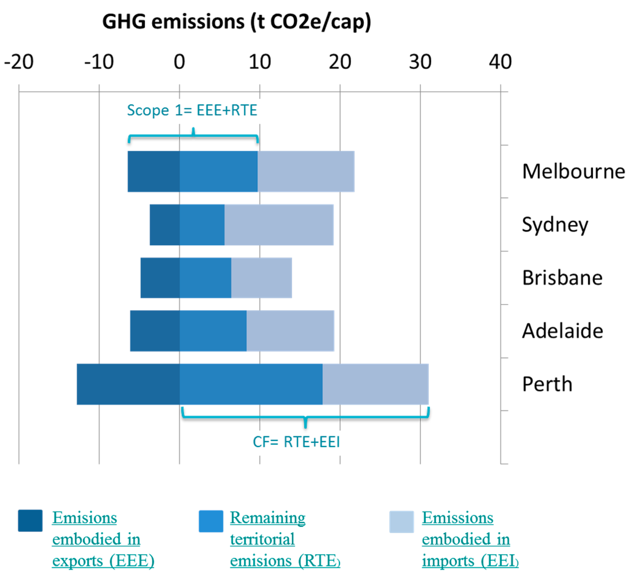
The analysis reveals several interesting aspects of embodied emission flows of cities. We define the city CF as a consumption-based measure that adds EEI to industry-related territorial emissions (also called scope 1 emissions, see C40, ICLEI and WRI [
22]) and subtracts EEE [
17]. Those scope 1 emissions that do not become embodied in exports are referred to as remaining territorial emissions (RTE). The results presented below (and our definitions of CF and RTE) do not include direct emissions from households coming from private transport and heating homes (there is no district heating in Australia). We report these emissions separately because they never become embodied in the supply chain of goods and services in the economy and are therefore not part of the network of embodied emission flows.
Perth has the highest per-capita CF (31 t CO
2e/cap) of the five cities studied, followed by Melbourne (22 t CO
2e/cap), Adelaide (19 t CO
2e/cap), Sydney (19 t CO
2e/cap) and Brisbane (14 t CO
2e/cap) (
Figure 1). Direct household emissions add another 2.2–3.3 t CO
2e/cap (not shown in
Figure 1, see
Supplementary Data, Supplementary Materials). In all cities, except for Perth, imported emissions are larger than the RTE of the city itself. This means that all cities, except Perth, rely more on GHG emissions from elsewhere in Australia and the world than from their own industries, to satisfy their final demand. This reflects the density and extent of supply chain networks that cities in the Eastern part of Australia rely on.
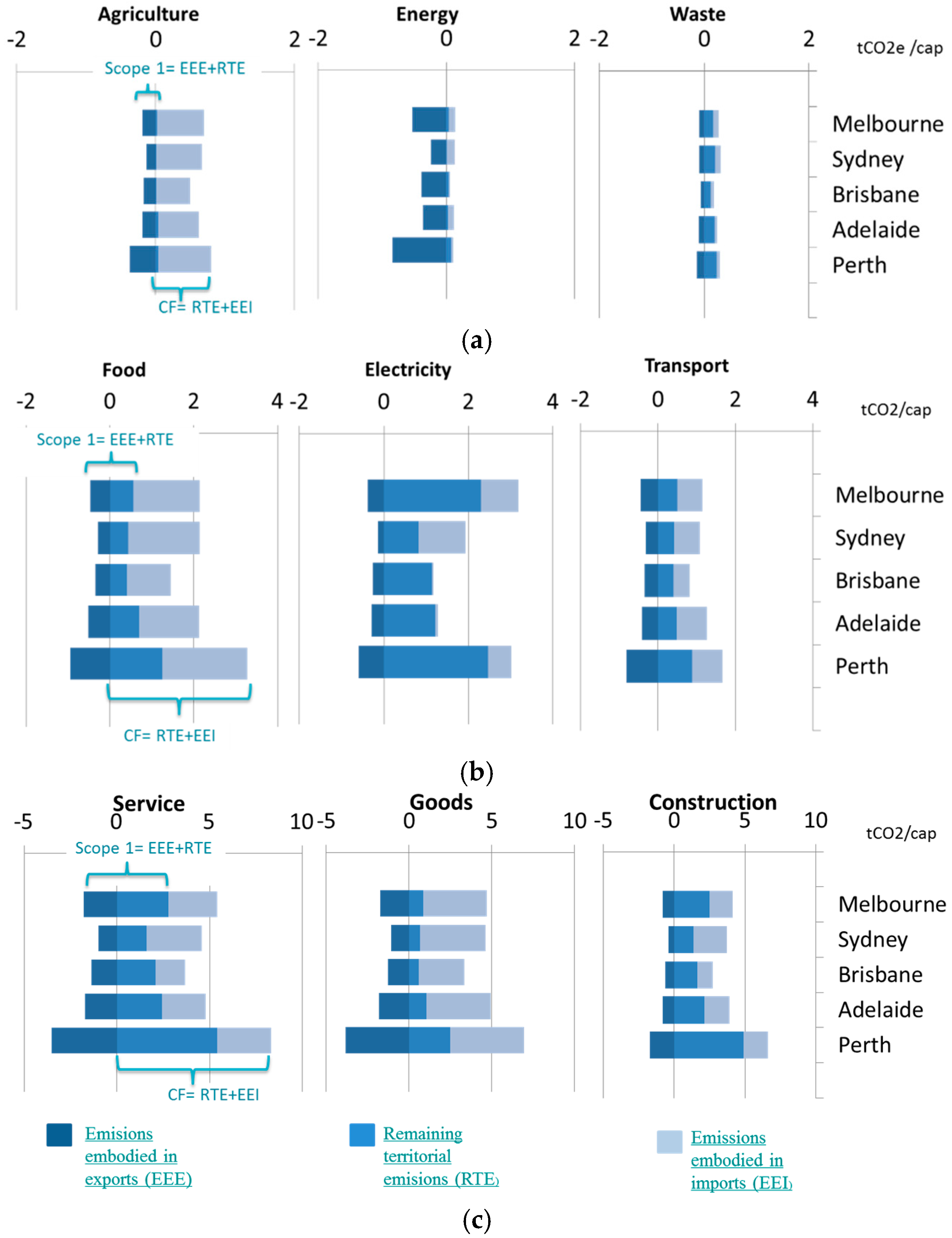
A breakdown by sector (
Figure 2, note the different scales in the graphs) reveals that the largest components of the city CF are generally attributable to final demand in five economic sectors: services, goods, construction, food and electricity. In all cities, the CF components for services and goods are the highest compared to other sectors.
In Melbourne, Brisbane and Adelaide, the RTE for services are slightly larger than EEI, making up 51%, 57% and 51% of the services CF respectively. This indicates that those cities meet just over half of their respective final demands for services by producing emissions within their own borders. The RTE for services in those cities are also larger than EEE, which indicates that the majority of emissions generated within the city border due to the supply of services are attributable to consumption within each city itself, rather than in response to external demand. In Sydney, RTE are about half the EEI and only represent 35% of the CF of services, while in Perth the RTE are about twice the EEI and represent 65% of the services CF. This indicates that Sydney is much more highly dependent on imports of embodied emissions to meet its demand for services than Perth is.
The goods sector also makes up a large proportion of city CF, at 3.4–7.0 t CO2e/cap. Melbourne, Sydney and Brisbane have more than 80% of their goods CF coming from EEI, while Adelaide and Perth have 78% and 64%, respectively. The EEE of goods contribute 1.1–3.8 t CO2e/cap, and are much larger than the RTE for all cities. The relatively small contribution of RTE to the CF of goods, despite the large EEE, is likely to reflect a mismatch between the types of goods (and their precursors, i.e., raw materials) demanded and produced by each city.
In the construction sector, the CF ranges from 3.7 t CO2e/cap to 6.6 t CO2e/cap, with the EEI making up 26%–63%. Perth has the largest construction CF per capita, much higher than the other four cities. This is despite the contribution of EEI (26%) being relatively small (due to Perth’s geographical isolation), suggesting a high volume of construction in this fast-growing city and/or the use of more GHG-intensive construction methods or materials are responsible for the large construction CF.
The food sector CF is 1.5–3.3 t CO2e/cap, with 62%–80% coming from EEI. In all cities, EEE are relatively small and EEI relatively high compared to the total CF. This is typical for large cities that rely on agricultural hinterlands to produce the majority of the food they consume. Again, Perth appears to be somewhat more self-sufficient in carbon terms, with about 38% of its food CF coming from its own territory (RTE).
For the electricity sector, the city CF ranges from 1.2 t CO2e/cap to 3.2 t CO2e/cap, with highly variable EEI between the different cities (Sydney 57% of CF, Melbourne 28%, Perth 18%, Adelaide 2% and Brisbane 1%). Because the CF of electricity is dominated by generation, this reflects the fact that Brisbane and Adelaide more rely on the generation of electricity within their own borders, while the other cities more depend on supplies from power stations further afield.
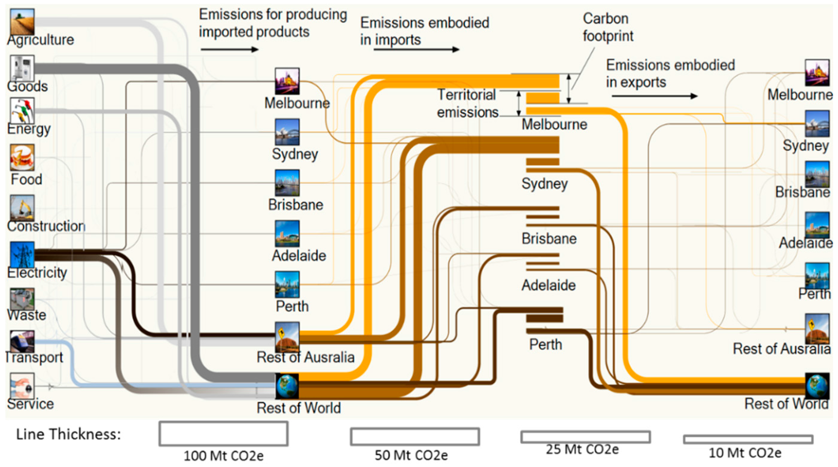
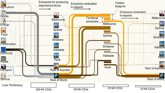
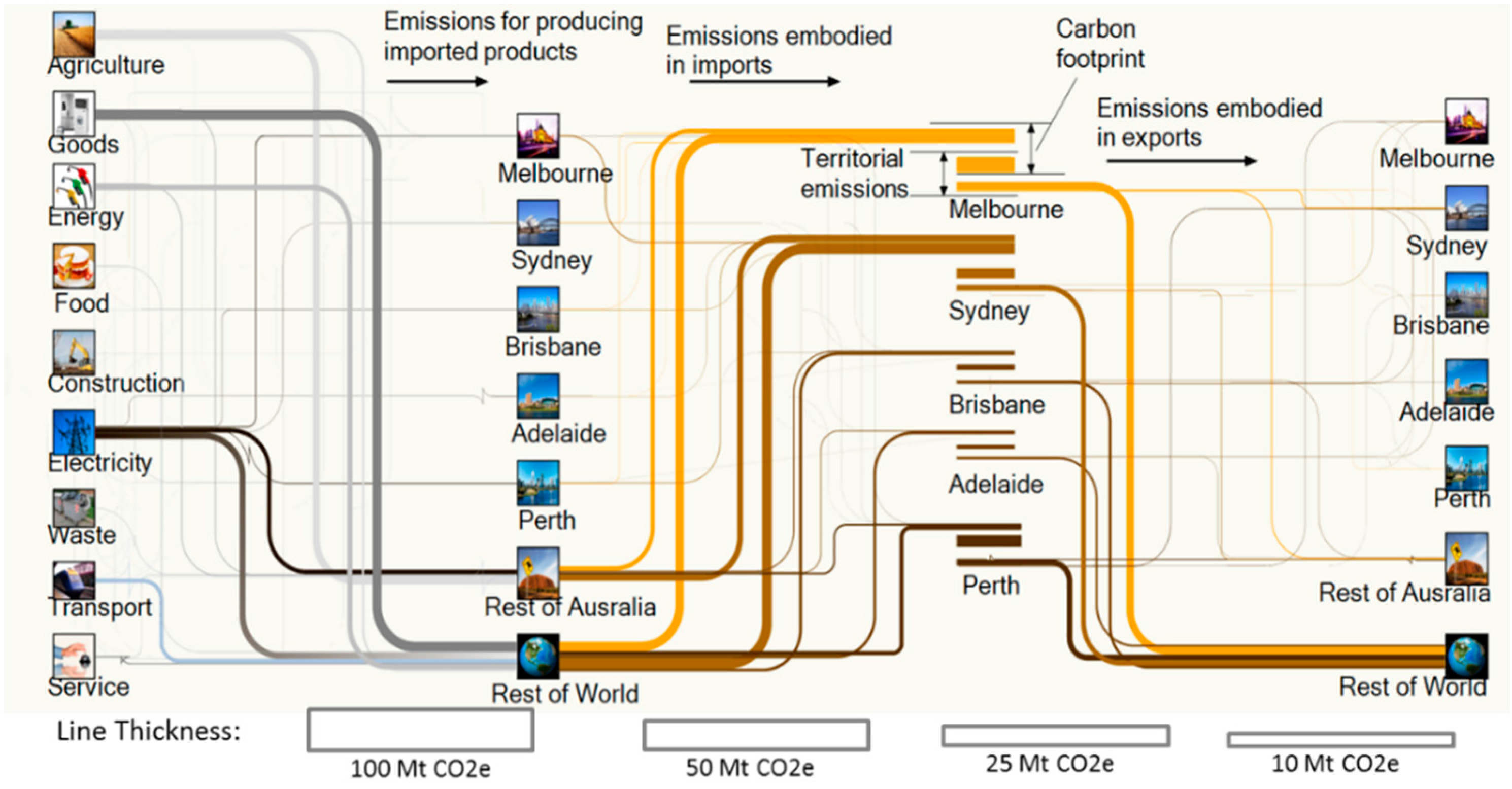
3.2. Total Carbon Footprint Networks
In the following section we show the flow of embodied GHG emissions between cities and regions broken down by sector. Reading from left to right, the flow diagrams (
Figure 3,
Figure 4 and
Figure 5) display the origin of emissions from economic sectors, the cities in which those sectors are located, and how the emissions become embodied in the final demand of other cities (centre of the diagram). The right-hand side of the diagram shows how territorial (scope 1) emissions from cities become embodied in other cities or regions. Note that all flows are virtual, i.e., GHG emissions are not actually transferred physically between the cities—they have only been reallocated from production (origin) to consumption (destination) [
20].
The majority of EEI for Australian cities comes from the Rest of World (RoW) region (55%–73%), with the remaining 22%–34% of EEI from the Rest of Australia (RoA) (
Figure 3). The EEI from the RoW region are mainly from goods (37%), electricity (21%), transport (15%) and energy (15%), whereas in the RoA region they are mainly from agriculture (51%) and electricity (31%). The EEE are sizeable compared to the cities’ CF (19%–41% thereof), but do not count towards a consumption-based CF. The RoW region receives 76%–83% of EEE from the five cities, reflecting the dominance of international over domestic exports.
Previous studies have found that trans-boundary emissions make up about half of a city’s total CF. For example, in the case of eight US cities, the boundary-limited GHG accounting methods appear to underestimate the overall GHG emissions impact of material and energy demand in cities by 47% on average, with most of the difference coming from air and freight transport plus emissions embodied in food, fuel, cement, and water/wastewater [
28]. For China’s four mega cities, 48%–72% of CF comes from EEI, mainly embodied in goods [
29]. Our results are similar, showing that EEI make up 71% of CF in Sydney, 54%–57% in Melbourne, Brisbane and Adelaide, and 43% in Perth.
At a national scale, 55% of the total Australian CF is due to the final demand of these five large cities, with around one quarter of the Australian CF attributable to these cities’ imports from overseas. As part of a specialised and globalised economy, Australian cities are drawing carbon and other resources from global supply chains by outsourcing production to the RoW region. They also outsource emissions to the RoA region, amounting to 22%–34% of EEI. In contrast, the direct links between the cities themselves are not as strong, as evidenced by the much smaller intercity carbon flows.
Responsibilities for territorial emissions are well understood in the recently released GHG Protocol for Cities [
22], but the trans-boundary emissions are not comprehensively reported, and have been largely ignored in climate policy. Applying the concept of city carbon maps allows us to trace emissions from individual industry sectors to final demand in cities. In the next section, the emissions embodied in the final demand of some specific sectors (columns in the city carbon map) are further analysed to unravel the trans-boundary emissions networks between regions and cities. Figures for the remaining sectors are presented in the
Figures S7–S13.
3.3. Carbon Footprint Networks by Sector
In the agriculture sector (
Figure S7) 74%–76% of EEI to the five cities originates from the rest of Australia, a result of Australia’s self-sufficiency in agricultural production. Exports from the agricultural sector are also strong, some of which are routed via the five cities to the RoW region, making up 47%–61% of the cities’ EEE. This is also confirmed by EEE in the food sectors where 75%–85% goes to RoW (
Figure S8).
In the electricity sector, 70% of Melbourne’s electricity emissions are exported to Sydney, while Sydney exported 59% of its own electricity emissions to Melbourne (
Figure S9). Brisbane, Adelaide and Perth export 33%, 32% and 35% of electricity emissions to Melbourne respectively, and 41%, 39%, 42% to Sydney. This highlights the importance of trans-local cooperation in mitigation policy, which should consider the exchange of electricity between cities. For other energy-related final demand, more than 90% of the five cities’ EEE goes to RoW.
With respect to manufactured goods, the RoW region supplies 85%–96% of the five cities’ EEI, while it also receives 91%–94% of their EEE (
Figure S10). This indicates that the five Australian cities rely much more on goods from RoW than from RoA or from each other. This reflects Australia’s status as a resource-rich country with an economy dominated by extractive sectors and exports of raw materials. Most manufactured goods are imported from overseas and most of the final demand for them is in cities.
In the construction sector, 19%–39% of EEI is from the RoA region while 44%–76% is from RoW as both construction materials and related services are imported from overseas (
Figure S13). The RoW region also receives 59%–73% of the EEE of construction from the five cities. Notably, 21%–25% of the EEE of construction goes to Sydney from the other four cities.
The flows of emissions embodied in the final demand for transport services show an interesting pattern (
Figure 4). The transport-related EEI of Melbourne and Sydney are larger than the RTE in these cities (in
Figure 4, RTE are represented by the middle bar in the stacks of city emissions, i.e., the overlap between CF and all territorial emissions). Furthermore, most of the EEI (82%–92%) across the five cities come from the RoW, while 90%–91% of transport EEE flow back to final demand for transport services in the RoW.
How can it be explained that the CF of transport services in Australian cities is dominated by embodied emissions from the rest of world and not by local transport emissions? Firstly, we need to recall that the flows in
Figure 4 only include industry-related emissions, i.e., from freight and public transport, and not from private transport. Adding the latter to the CF in all cities increases the RTE of transport substantially, e.g., from 2.0 Mt CO
2e to 9.7 Mt CO
2e in Melbourne and from 1.8 Mt CO
2e to 11.1 Mt CO
2e in Sydney (numbers for all cities are provided in the
Supporting Data (SD) spreadsheet). With direct emissions included, the EEI share of the total transport CFs across the cities drops to 13%–22%. Secondly, some transport services are provided by internationally-based companies that report their emissions outside Australia (e.g., foreign airlines) or by international carriers collaborating with (and paid for by) domestic transport companies.
In the service sector, 22%–33% of the EEI of the five cities are from RoA while 56%–74% are from RoW. The upstream emissions caused by the EEI of service vary from region to region. The largest contribution is from the electricity sector (51%–67%, both from RoA and RoW) and from the goods sector (4%–34%, mostly from RoW) which indicates that the provision of services to the five cities relies heavily on electricity and manufactured goods from further upstream in the global web of supply chains [
57]. Most of the EEE of the five cities goes to RoW (75%–82%), while 9%–11% goes to RoA. This reflects the international export orientation of some services offered in the cities, e.g., tertiary education. As the city with the largest imports, Sydney also receives 8%–9% of the other four cities’ EEE, followed by Melbourne (4%–5%).
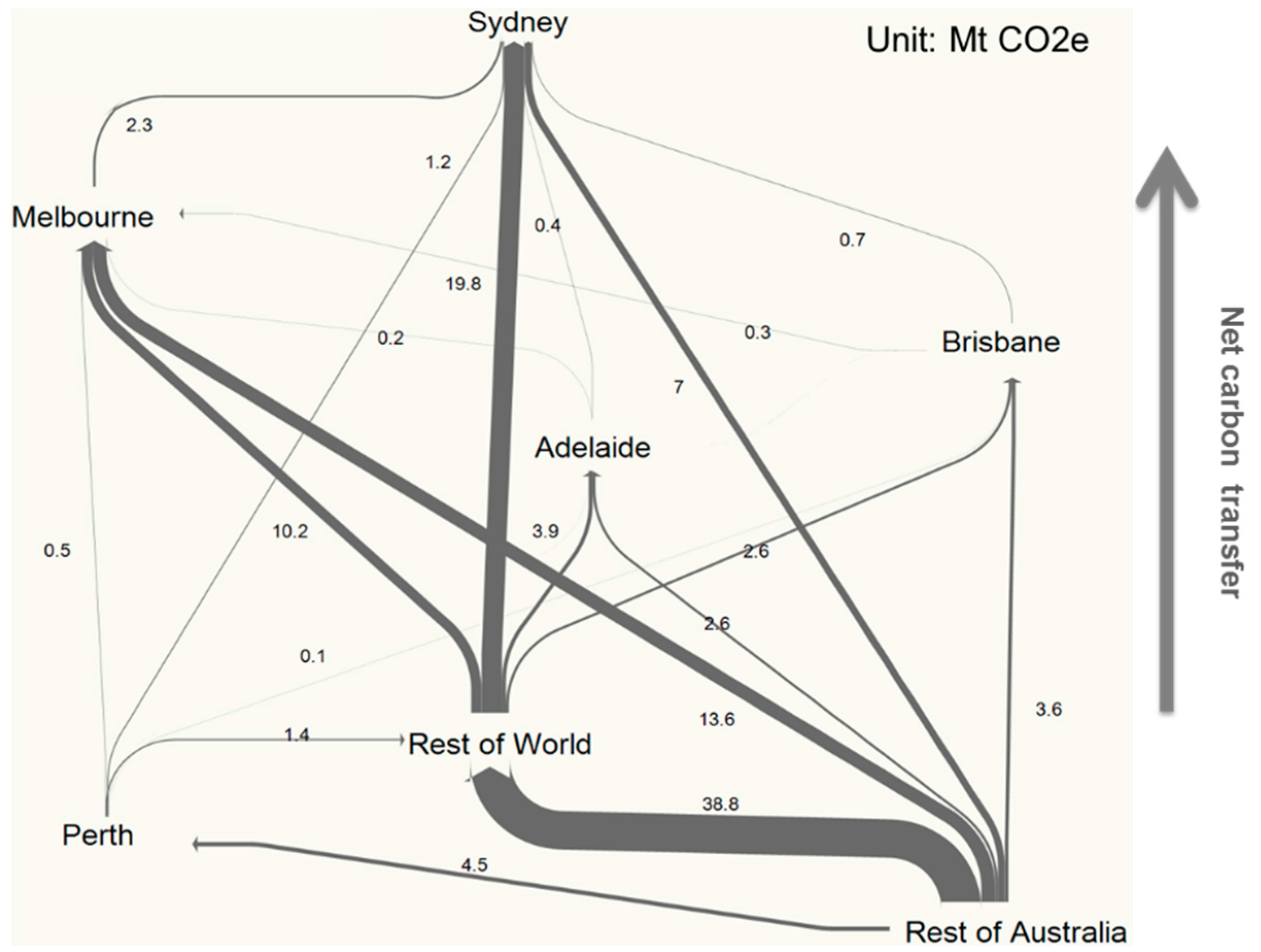
3.4. Balance of Emissions Embodied in Intercity Trade
The consumption-based analysis also allows for a differentiated perspective on the responsibility of cities for GHG emissions. For example, some cities have relatively small per-capita emissions within their own territory, but are actually driving emissions-producing activities in other regions through the net import of embodied emissions (EEI − EEE).
Figure 6 shows a hierarchy in which Sydney, as the largest driver, is the main net importer of GHGs from other territories (net emission flows go from bottom to top). Sydney’s net EEI mainly come from RoW (63%) and RoA (22%) with 7% coming from Melbourne and the remainder from the other cities. In contrast to Sydney, Melbourne (the second-largest driver) has more net EEI from RoA (55%) than from RoW (41%). Brisbane and Adelaide are the third and fourth largest drivers. Notably, Perth has larger EEE compared to EEI from the RoW, which makes it the only one of the five cities to be a net international exporter of emissions. The RoA is at the lowest level of the hierarchy and is “serving” all of the cities and the RoW with embodied emissions (through the export of resources and materials). The international and intra-national flows of emissions embodied in trade with geographical information can be obtained in
Figure S14.
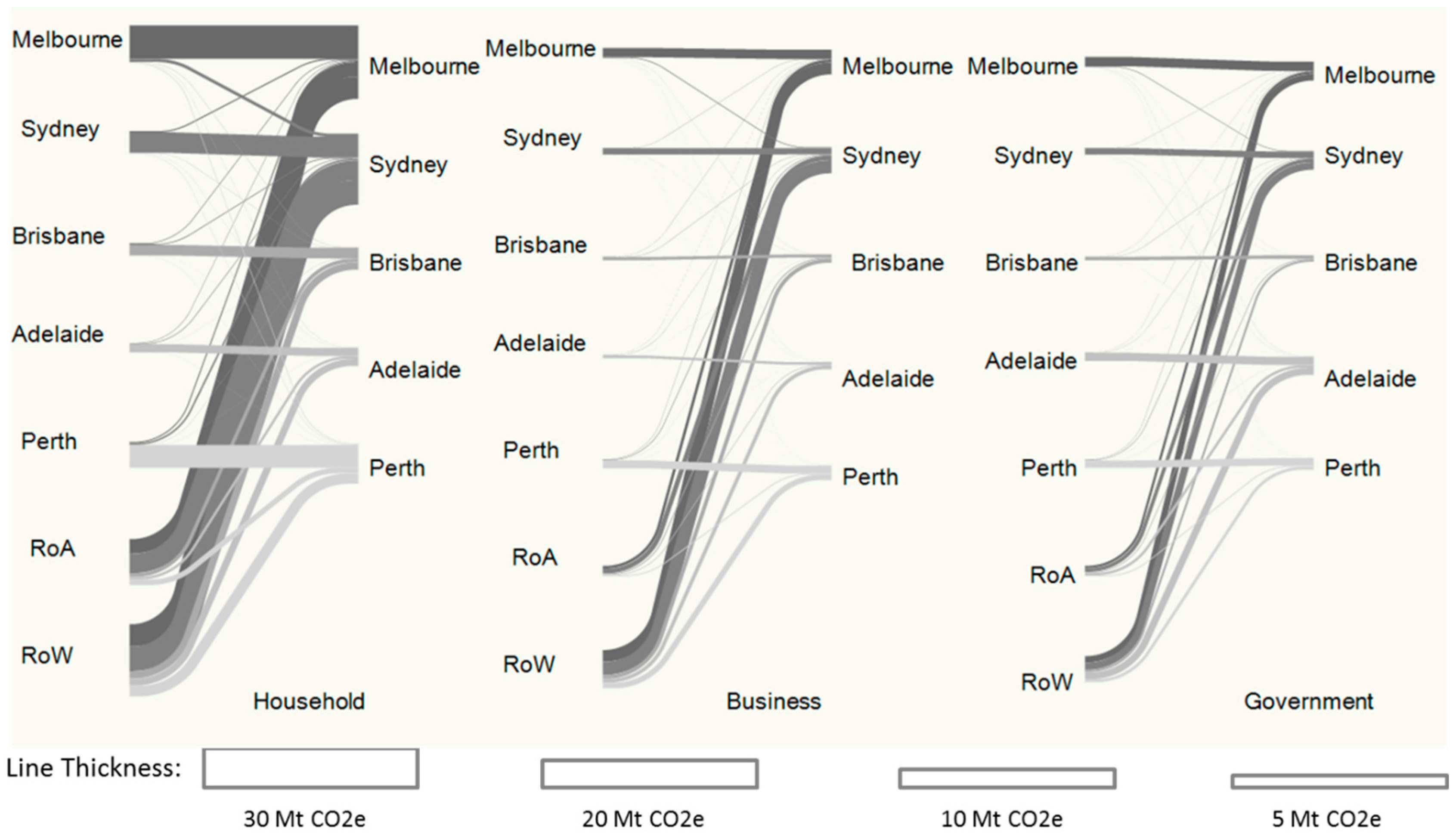
3.5. Emissions Allocated to Households, Business and Government
When looking at the components of final demand (
Figure 7) household consumption makes up the majority (59%–63%) of total city CF, followed by business and government final demand ( 21%–24% and 16%–17% respectively).
Of the emissions driven by household consumption, 29%–57% originate within the city territory, with 14%–27% from RoA and 26%–38% from RoW. A slightly lower percentage of the emissions driven by business consumption originate within the city boundary (24%–54%), more are from the RoW (39%–51%), and only 6%–18% are from RoA. Emissions driven by government consumption originate 35%–64% from within the city territory, 26%–39% from RoW and 8%–19% from RoW.
In summary, an average of 60% of carbon emissions is due to the consumption of households, while business and government consumption accounts for a combined 40%. Business consumption tends to outsource its emissions to the rest of the world, while government and households have higher emissions within the city boundary, which may lead to different mitigation policy implications. The detailed breakdown of emissions sources also varies by city. For example, household-related emissions within Melbourne mainly originate from territorial electricity generation, while in Sydney they are mainly driven by demand for services.
3.6. Uncertainties and Limitations
This work has several uncertainties and limitations associated with its origins in MRIO analysis. All values of economic transactions and embodied carbon flows are imputed top-down, using proxy data and location quotient methods for the regionalisation of data [
49]. We offer the following suggestions to improve on our analysis in future work:
Sourcing and using locally specific data as well as adapting the regionalisation procedure in the IELab, both for IO data and for GHG emissions data, to the specific situation of cities.
Scope 1 and scope 2 emissions would be more precise if they were collected bottom-up rather than derived by economic (proxy) allocation.
Highly disaggregated sectors are recommended if the data are available; because sectors are quite aggregated in this study, some intricacies of trade in products are lost through averaging.
This analysis considers only three GHGs (omitting, for example, CFCs/HFCs related to cooling), and could be expanded if data on more emissions substances become available.
For simplicity, the final demand categories of “changes in inventories” across various sectors were fully allocated to business final demand. However, for some sectors there might also be a substantial change in inventories due to government expenditure.
We adjusted the RoW data using an international MRIO model (Eora [
58,
59,
60]) that makes several assumptions as detailed in [
20]. This could be improved through the use of primary trade data if available.
The RoW region could also be further subdivided into different countries to reveal bilateral emissions flows between Australian cities and other countries [
17].
4. Discussion and Conclusions
More than half of the Australian national CF is attributable to consumption in the five large city studies, with many of those GHG emissions embodied in international imports of goods and services. Neglecting this latter part of emissions would lead to underestimation of the national CF in the order of one quarter. This suggests that the current focus on territorial emissions would be ineffective at reducing city, national and even global emissions in the absence of mechanisms to monitor and report emissions embodied in imported goods and services. Whilst cities are traditionally seen as drivers of emissions, there are already signs that cities can act as frontrunners of positive change in this respect [
1].
CBA should routinely be adopted by cities, with both the emissions embodied in imports and exports well monitored [
8], especially for embodied emissions of goods and services that have been shown to make up substantial parts of city CFs. This would complement the approach focused on scopes 1 and 2 already implemented by most current city carbon accounting standards [
54,
61]. Note that CBA extracts EEEs from the city inventory, which does not mean, however, that cities are exonerated from these emissions and no longer responsible. On the contrary, CBA reinforces the need to recognise and act on shared responsibility [
62]. The carbon flow network analysis presented in this paper can help with the design of comprehensive mitigation strategies involving trade partners. The absence of particular mechanisms to force cities to account for out-of-boundary emissions in a comprehensive manner in part originates in the lack of quantification mechanisms for such carbon flows—a gap which the present study has contributed towards addressing.
For the five cities studied, we find that services, goods, electricity, food and construction are the final demand sectors that drive the highest emissions. Though the originating sector, composition and provenance of the embodied emissions in these sectors vary significantly from region to region, some low-hanging fruits for mitigation can be identified. The shift of consumption from coal-based electricity to renewable energy plays a key role. For example, Melbourne’s electricity sector makes up about one quarter of its territorial emissions. Mitigating the emissions from the electricity sector will also benefit the service and construction sectors in all five cities as they are all heavily reliant on electricity.
Households are responsible for about two thirds of the city CFs, while government and business drive the remaining one third. Reducing GHG emissions by promoting low-carbon household behaviours changes has been discussed in literatures [
63,
64,
65,
66]. Similar programmes could be set up for public and private spending and investment. Besides market-based mitigation policies, such as emissions trading schemes or carbon taxes, pledges for mitigation made by cities should be encouraged. A ranking system like the Climate Action Tracker tool could be used to evaluate the degree of implementation for each climate action [
67]. This would help to compare and identify actions that are actually being carried out and those that exist only on paper [
8]. Government funding could be used to incentivise the achievement of high ranks in the tracker.
The major driving forces behind national emissions in developed countries are large cities. We have demonstrated a hierarchy in which the five major cities, with the exception of Perth, are net importers that also drive international emissions. Perth has the highest per-capita emissions of the five cities, and “serves” international final demand through net GHG exports, particularly from the energy sector. In contrast, Sydney has the second-lowest per-capita CF, but it is at the top of the hierarchy and outsources the emissions to all other domestic regions as well as abroad.
The hierarchy suggests a responsibility dividend for cities and could become an incentive that drives low-carbon outcomes through carbon trading among cities. Cities could guide the trade in carbon credit units in a way that lowers not just their territorial but also their imported emissions. To illustrate, as a net importer from Melbourne, Sydney could require or support companies to purchase credit units from Melbourne, as improving carbon efficiency in Melbourne will also lower the EEI to Sydney. In Perth, an emission-exporting city at the bottom of the hierarchy, territorial emissions reductions could be sold as carbon credits to the rest of Australia and the world, if there was an appropriate carbon market. The findings presented in this study thus highlight the importance of quantifying and understanding inter-regional and inter-city carbon flows. These provide a holistic assessment of GHG origin and responsibility but also stress the significant heterogeneity that exists between different cities, even within the same country. The policy recommendations thus need to be tailored to the city context.
Consideration of these aspects also informs the debate about emissions responsibility and promotes collaborative actions for climate change mitigation. For multi-city collaborations on mitigating emissions is more than common target setting and information sharing. Carbon trading can cover cities as much as states and nations. As the world’s first urban trading system, the Tokyo Cap-and-Trade Program, focusing on regulating emissions from urban facilities such as office buildings, has achieved a 25% reduction of emissions since 2010 [
68]. China launched its pilot schemes and traded emissions among five cities and two provinces since 2011 [
69]. Québec and California pioneered the linking of a regional carbon market on the premise that extended carbon markets induce greater GHG emissions reductions and drive down the overall cost of mitigation [
70].
Australia’s Emission Reduction Fund Safeguard Mechanism was set to commence on 1 July 2016 [
71]. The Government’s current policy position is that Australian Carbon Credit Units (ACCUs) are the only prescribed carbon units that can be used [
71]. The offshore unit option is ruled out by the policy since it does not fit with the interests of domestic emitters. However, offsets invested in countries where imported emissions originate could help in reducing emissions from outside the national territory and are also likely to be cheaper than national offset projects [
72]. The lack of a carbon market in Australia also hinders the global private sector from accessing Australian carbon credit units. In the absence of any mechanism to encourage investments from cities to reduce their out-of-boundary emissions, the potential of creating positive knock-on effects is significantly diminished. This has been realised by governors in the Paris climate conference, and clearer rules around the trading of international carbon credits may be provided after 2020 [
73].
Within the constraints of limited budgets, technical expertise and human resources, Australia could first test a carbon market in the five capital cities by drawing from experiences in other countries like China, where seven pilot carbon trading schemes have already been established to cover five cities and two provinces [
69]. Later on, domestically approved carbon credits could be expanded to include international unit options.
In conclusion, based on the concept of city carbon networks, mapping out trans-city flows of embodied carbon emissions as carried out in this study, not only provides a better understanding of the hinterland effects of urban consumption, but can also guide investment and trading strategies under market-based emission reduction schemes, especially with regards to identifying upstream “hotspots” for city carbon mitigation. Guiding carbon trading through domestic and international markets by matching it with efforts to achieve city carbon neutrality could increase the speed and efficiency of both national and global carbon reductions.


