Electricity Price Forecasting by Averaging Dynamic Factor Models ^†

Abstract

In the context of the liberalization of electricity markets, forecasting prices is essential. With this aim, research has evolved to model the particularities of electricity prices. In particular, dynamic factor models have been quite successful in the task, both in the short and long run. However, specifying a single model for the unobserved factors is difficult, and it cannot be guaranteed that such a model exists. In this paper, model averaging is employed to overcome this difficulty, with the expectation that electricity prices would be better forecast by a combination of models for the factors than by a single model. Although our procedure is applicable in other markets, it is illustrated with an application to forecasting spot prices of the Iberian Market, MIBEL (The Iberian Electricity Market). Three combinations of forecasts are successful in providing improved results for alternative forecasting horizons.

1. Introduction

Nowadays, electricity trading is liberalized in most countries of the Western world. Due to the particular characteristics of supply and demand, the prediction of electricity prices in this context is complex. Notwithstanding the difficulties, forecasts are necessary for several reasons:

• this is a strategic sector of the economy;
• there are financial implications due to the trading of forwards and options;
• forecasts help optimize and plan consumption and production.

As with other commodities, there are various ways to operate in this market (see [1] for a detailed market description and a thorough literature review). We focus on prices that result from a pool in which there is a central auction. In this pool, prices could be settled for each hour of the day, or every half hour, depending on the market.

In the first case, the 24 hourly prices for day t are cleared at the same instant in day t − 1, with the same common information for all of the hours. Therefore, for each day, a 24-dimensional vector is generated $(p_{1,t},p_{2,t},\dots ,p_{24,t})$; where $p_{h,t}$ represents the price of hour $h=1,2,\dots ,24$ at day t. Consequently, prices can be presented in a $T\times 24$ dimensional matrix, where T is the number of days in the sample, and modeling should be multivariate (as in [2,3,4,5]).

In several fields, there has been an increasing interest in the development of a methodology to deal with multivariate time series or a high dimensional vector of series. By the end of the 1970s, [6] (these authors presented a factor model for stationary time series vectors) and [7] were the first to propose a dynamic factor model. Later, [8] contributed by extending the idea of principal components to the dynamic case. More recently, dimensionality reduction techniques have gained popularity, in particular since the work by [9]. For example, [10,11] extended [6]’s model for the non-stationary case.

Regarding applications in electricity markets, [12] extended [8,13] to prices with seasonality. Working with data for the Iberian market for 2007–2009, they propose extracting common factors from the 24-dimensional price vector and modeling such factors as univariate seasonal AutoRegressive Integrated Moving Average (ARIMA) processes. The work in [5] proposes a technique called Seasonal Dynamic Factor Analysis (SeaDFA), which involves the estimation of a Vector AutoRegressive Integrated Moving Average (VARIMA) model for unobserved common factors having seasonal patterns. The work in [14] also uses a factor model, including not only hours, but also locations.

In an independent path, forecast combination or model averaging has been developed as a technique to take advantage of the availability of alternative forecasting approaches. This methodology consists of weighting a set of forecasts corresponding to alternative models and combining them to obtain a single forecast. In this way, model selection uncertainty is incorporated. According to [15], “the idea of combining forecasts implicitly assumed that one could not identify the underlying process, but that different forecasting models were able to capture different aspects of the information available for prediction”. Other justifications for model averaging are: doubts of the existence of a “best model” [16], “portfolio diversification”, a better adaptation to structural breaks or to average out omitted variables’ bias [17].

Applications of model averaging in electricity markets are given by [18] (for the British market) and [19] (for European and USA markets). Furthermore, [20] obtain forecasts for the daily average price employing dimensionality reduction techniques, as well as the forecast combination of several models for hourly prices. Other references are [21], who use averaging to obtain wind speed, solar irradiation and temperature forecasts, which are employed to estimate prices; and [22], who forecast hourly electricity prices for the Spanish market by weighting seasonal ARIMA (with exogenous variables) and seasonal dynamic factor models of similar performance.

A major drawback of dimensionality reduction techniques is the uncertainty regarding the “correct” model: how many factors to include, and what models they follow. The literature is not definite in regards to the best technique for estimating the number of underlying factors that would contain enough information to make accurate predictions, considering that, as the number of factors included increases, so does estimation complexity and computational burden. As previously indicated, there is no unique model for these factors that outperforms all other models in all circumstances [1].

In this work, it is hypothesized that the major decisions attached to forecasting by using dimensionality reduction techniques may be resolved in a less arbitrary way if forecast combination is included. In order to follow this course, alternative models, including different numbers of common factors, are estimated. Forecasts are obtained by transforming the factors’ forecasts back to the data units, according to the relations established in the dimensionality technique employed. Subsequently, forecast combination approaches are used to weight each of the forecasts obtained and, thus, to provide a single prediction.

Summing up, factor models extract information ex ante (before any forecast is obtained), while forecast combination works ex post (after forecasts are available). The contribution of this work is to amalgamate both techniques. A reduced number of latent unobserved variables is estimated, and their forecasts are combined in order to obtain a single prediction.

We apply these techniques to one-day-ahead electricity prices for the Iberian spot market for a period of five years. Several ARIMA specifications (for each one of the common factors included in the analysis, 36 choices of parameters are available: $p=1,2,3$, $d=0$, $q=1,2,3$, $P=0,1$, $D=1$, $Q=0,1$, $s=7$; these pre-defined models are all automatically estimated with the software TRAMO, by its MATLAB interface, intervening outliers.) are estimated for the factors and used to obtain forecasts of the prices for each hour, which makes the task computationally intensive. Next, these forecasts are combined. We study alternative ways to combine forecasts because their performance may vary depending on the dataset. The predictions concern mainly the short- and medium-term (one and two months), but a one-year extension is presented to illustrate the potential accomplishments in long-term forecasting.

The rest of the paper is organized as follows. Fundamentals containing a mathematical description of the proposed methodology are presented in Section 2, which includes definitions on dynamic factor models, classical techniques for forecasts combination and Bayesian model averaging. Section 3 describes the methodology for this paper. In Section 4 , we present the results of the empirical application. This section is divided into sub-sections presenting the data, an analysis of variance (ANOVA) comparing specifications, and forecasting results. Finally, Section 5 concludes with remarks, limitations and possible extensions.

2. Fundamentals

An outline of the methodology used in this proposal is presented below, as are the drawbacks of other approaches, which we attempt to resolve.

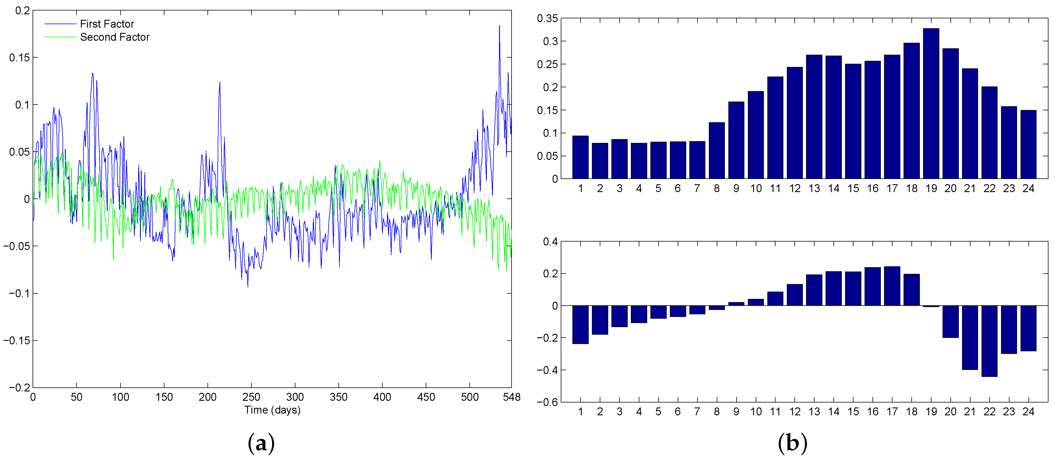
2.1. Dynamic Factor Model (DFM)

Dynamic Factor Models (DFM) are a widely-applied dimensionality reduction technique. It is employed when the researcher believes there are fundamental factors driving several variables in a dataset. These factors, like the variables, evolve through time and allow one to obtain information about the larger dataset with a simpler model. The explanation here follows [12]. As there, once the common factors are obtained, univariate seasonal ARIMA models are fitted to them. The forecasts of these models are then combined to obtain one improved forecast.

Let $y_t$ be an m-dimensional observed time series vector, generated by an r-dimensional vector of unobserved common factors $r\ll m$. In the Iberian electricity market $m=24$, and the matrix of observed series has as many rows as days are considered in the historic dataset. As in [8], it is assumed that vector $y_t$ can be written as a linear combination of the unobserved common factors $F_t$, plus a vector of specific components or factors ${\epsilon }_t$:

$$y_t=\Omega F_t+{\epsilon }_t$$

(1)

where Ω is an $m\times r$ matrix of loads relating the set of r common unobserved factors with the vector of observed series $y_t$ (the vector of the 24 hourly prices for our application) and ${\epsilon }_t$ is an m-dimensional vector of specific components.

To estimate the factors $F_t$, singular value decomposition (SVD) is used (as in [8]) for the covariance of the 24 dimensional vectors of centered prices [12]. This consists of calculating the eigenvalues, and their associated eigenvectors, for the sample covariance matrix, and thereupon calculating the matrix of common factors, $\widehat{F}$, as a linear combination of the time series: ${\widehat{F}}_{T\times r}=Y_{T\times m}{\widehat{\Omega }}_{m\times r}$. $\widehat{F}=[{\widehat{F^{\prime }}}_1,{\widehat{F^{\prime }}}_2,...,{\widehat{F^{\prime }}}_T]$ has dimension $T\times r$, where T is the length of the period employed in estimation and r the number of common factors in the analysis.

$F_t$ may be non-stationary, including regular or seasonal unit roots in addition to auto-regressive and moving average (regular and seasonal) components. These ARIMA$(p,d,q)\times (P,D,Q)s$ models are used to obtain factors’ forecasts and from them, prices’ forecasts. For instance, the i-th factor at date t, ${\widehat{F}}_{it}$, would be modeled by:

$${(1-B)}^d{(1-B^s)}^D{\varphi }_i(B){\Phi }_i(B^s){\widehat{F}}_{it}=c_i+{\theta }_i(B){\Theta }_i(B^s)w_{it}$$

(2)

where $i=1,2,\dots ,r$ is the i-th factor, ${\varphi }_i(B)=(1-{\varphi }_{i1}B-{\varphi }_{i2}{B}^2-\dots -{\varphi }_{i{p}_i}{B}^{p_i})$, ${\Phi }_i(B^s)=(1-{\Phi }_{i1}{B}^s-{\Phi }_{i2}{B}^{2s}-\dots -{\Phi }_{i{P}_i}{B}^{P_{i}s})$, ${\theta }_i(B)=(1-{\theta }_{i1}B-{\theta }_{i2}{B}^2-\dots -{\theta }_{i{q}_i}{B}^{q_i})$ and ${\Theta }_i(B^s)=(1-{\Theta }_{i1}B-{\Theta }_{i2}{B}^{2s}-\dots -{\Theta }_{i{Q}_i}{B}^{Q_{i}s})$ are polynomials; B is the lag operator, such that $B{y}_t=y_{t-1}$. The roots of $|{\varphi }_i(B)|=0$, $|{\Phi }_i(B^s)|=0$, $|{\theta }_i(B)|=0$, $|{\Theta }_i(B^s)|=0$, satisfy the usual stationarity and invertibility conditions, and $w_{it}\sim N(0,W_i)$ are uncorrelated $E(w_{it}{w}_{it-h}^{\prime })=0,h\ne 0$. It is also assumed that the error term of the common factors $w_{it}$ is uncorrelated with the specific components $E(w_{it}{\epsilon }_{t-h}^{\prime })=0,\forall h$. $c_i$ is the constant of the model for the common factors, and its inclusion in the common factors model in Equation (2) can be particularly relevant to calculate long-term forecasts in the non-stationary case (which is the case of electricity prices). Furthermore, in this work, the specific components are assumed to be independent and have no dynamic structure along them (e.g., [11]).

It should be noticed that the procedure of estimating the factors is independent of the procedure of estimating the ARIMA models. That is, first the factors’ estimates $\widehat{F}$ are obtained, and afterwards, the ARIMA models are estimated ($\widehat{\varphi },\widehat{\Phi },\widehat{\theta },\widehat{\Theta }$). Moreover, the estimation of the first factor is the same when $r=1$ or $r>1$, which is a natural consequence of the SVD procedure. Nevertheless, the selection of r acts on the value of the forecasting errors for the series. The more factors are included (greater r), the greater the variability of the data explained by the model. The cost of incorporating more factors is an increase in the number of parameters to estimate.

To summarize, a key stage when estimating this kind of model is the selection of the number of common factors, r, as well as the model they follow, which implies selecting the orders: $p,d,q,P,D,Q$. r could be obtained using the test proposed in [11] and could also be selected such that diagnostic checking results (specific factors and errors of the observation equation must be uncorrelated between them, and specific factors without any cross correlation) are reasonable [5]. However, alternative values could satisfy these criteria. Because selecting one value for r and the other parameters will likely not render the best results in every scenario, we will instead keep the alternatives and combine their forecasts. Forecast combination is presented in the following Subsection 2.2.

2.2. Forecast Combination

Empirically, the improvements of using forecast combination instead of a “best” model have been shown for different types of models (for instance, see [23,24,25]) and in various research areas [15,26]. However, [1] points out that forecast combination techniques have not been fully exploited for electricity prices.

In general, we can think of the combination equation as follows:

$${\widehat{y}}_{t+h|t}^C=\sum _{i=1}^K{w}_{ti}^{(h)}{\widehat{y}}_{t+h|t}^{(i)}$$

(3)

where $w_{ti}^{(h)}$ is the i-th model weight at time t for the forecast horizon h, K the total number of models considered and ${\widehat{y}}_{t+h|t}^{(i)}$ the forecast obtained with the i-th model for the forecast horizon h.

Combinations will vary depending on the weights they use and the set of models they include. There are classical and Bayesian techniques. In the next subsections, we briefly summarize the literature on both the classical approach and an approximation to Bayesian combination, mentioning their drawbacks and advantages. This will help us justify our methodological proposal presented in Section 3.

2.2.1. Classical Techniques for Forecast Combination

One easy way to obtain forecast combination is the simple average, in which all alternative forecasts are given the same weight. This approach often works very well in comparison with more complex ones. One possible reason is that “complicated combining methods pursuing “optimal” behavior often lead to unstable weights and the combined forecast even performs significantly worse than the individual forecasts” [27]. Alternatively, a simple combination method outperforming more complex ones might be explained by a larger variability of the latter [27]. In this regard, [17] advise to use a simple average when the alternative models to combine have similar forecast error variance.

A different approach to assign weights consists of estimating weights that minimize a loss function with the forecast error of the models to combine as explanatory variables [28].

A further option is a combination using only the $d_m$ best models. The possible advantages of this approach are: to reduce the variability of the combination [27] and to avoid under-weighting independent information when the models are correlated [17]. The set $d_m$ could change through time depending on the most recent performance of the models [17] (these authors evaluate model performance based on the sum squared errors; the results they obtain with a time-varying subgroup of models outperform those of the simple average of all of the models) or it could be fixed [29].

Another way to combine forecasts would be to employ the median prediction [24]. Alternatively, some authors employ a combination regression of the form:

$$\begin{array}{c}\hfill y_{t+h}={\alpha }_0+\sum _{i=1}^P{\alpha }_i{p}_{i,t}+{ϵ}_{t+1}\end{array}$$

where $y_{t+h}$ is the forecast resulting from the combination and $p_{i,t}$ are the predictions of the alternative models. The work in [29] uses the Bayesian information criterion (BIC) [30] or the Akaike information criterion (AIC) to select the best combination. There are also some drawbacks to this regression-based approach. The work in [29] indicates collinearity in the competing forecasts and over-fitting due to outliers; [31] adds that while in-sample fit is improved, out-of-sample prediction tends to be worse than using the average to combine.

Even using complex combinations, the empirical findings in [29] suggest that in some cases, the difference between alternative combination methods is not significant, a result that will also be obtained at points in this work.

2.2.2. Bayesian Techniques for Forecast Combination (BMA)

With this approach, the predictive distribution of a new observation is obtained by averaging with different weights the predictive distribution of each model considered. The idea was initially introduced by [32] and allows one to incorporate the uncertainty regarding the variety of available models [32]. It has been applied in statistics [33,34,35] and econometrics [36,37].

According to [31], an advantage of Bayesian Model Averaging (BMA) is that “One does not have to be a subjectivist Bayesian to believe in the usefulness of BMA, or of Bayesian shrinkage techniques more generally. A frequentist econometrician can interpret these methods as pragmatic devices that may be useful for out-of-sample forecasting in the face of model and parameter uncertainty”.

As [31] explains, the procedure takes under consideration a large number of alternative models’ forecasts, assuming one of them is the “true” data-generating model; however, the researcher is unaware of which one is this. A prior regarding which model is the correct one is set, and then, a posteriori probabilities of the different models being the true one are obtained to weight the predictions.

Alternative models’ weights can be time evolving. For instance, [38] work with weights that change depending on the predictive densities past performance and learning mechanisms.

Following [31]: let K be the total number of models $M_1,\dots ,M_K$. The i-th model is related to the vector of parameters ${\theta }_i$. The researcher has a priori knowledge of the probability that the i-th model is the true one, $p(M_i)$. Then, the data, D, are observed, and the probability is updated by calculating the a posteriori probability that model i-th is the true one:

$$p(M_i|D)=\frac{p(D|M_i)p(M_i)}{{\displaystyle \sum _{i=1}^K}p(D|M_j)p(M_j)}$$

(4)

where $p(D|M_i)=\int p(D|{\theta }_i,M_i)p({\theta }_i|M_i)d{\theta }_i$ is the marginal likelihood of the i-th model, $p({\theta }_i|M_i)$ is the a priori density of that model parameters’ vector and $p(D|{\theta }_i,M_i)$ is the likelihood. Inference about a “future” quantity Δ is based on:

$$p(\Delta |D)=\sum _{i=1}^{K}p(\Delta |D,M_i)p(M_i|D)$$

(5)

In particular, the mean of this posterior distribution is used as the forecast. This procedure minimizes the mean squared forecast error (MSFE). It is only necessary to specify the set of models, their priors $p(M_i)$ and the parameters’ priors $p({\theta }_i|M_i)$.

A disadvantage of this approach, though, is that the conditional probabilities are, in general, unknown. Therefore, they should be estimated from the data, which could mean that any benefits of forecast combination are lost.

Often, all models will have equal a priori probabilities, i.e., $p(M_i)=1/K$. In this case, as [33] indicates, the posterior probability $p(D|M_i)$ is proportional to $\exp (-(1/2)BI{C}_i)$. Therefore, Equation (4) can be written as follows,

$$p(M_i|D)\approx \frac{\exp (-(1/2)BI{C}_i)}{{\displaystyle \sum _{i=1}^K}\exp (-(1/2)BI{C}_i)}$$

(6)

Equation (6) is easy to calculate, and no prior densities need to be set [33]. In this paper, one of the forecast combinations will use weights obtained as indicated in equation (6).

Notice that the selection of equal a priori probabilities is motivated by the approach of using non-informative a priori probabilities. However, other a priori probabilities can be considered, and in such cases, Equation (6) would be:

$$p(M_i|D)\approx \frac{\exp (-(1/2)BI{C}_i)p(M_i)}{{\displaystyle \sum _{i=1}^K}\exp (-(1/2)BI{C}_i)p(M_i)}$$

(7)

In this paper, the goal is to derive some feasible and reasonable weights, not to estimate conditional probabilities. Of course, it is to be expected that clever a priori probabilities produce better weights in the sense of better forecast performance.

3. Methodology

Taking into account the limitations of existent approaches in dimensionality reduction, most importantly the issue of selecting a number of common underlying factors r, as well deciding for a “best” model for them, and given the advantages of forecast combination revisited in the previous sections, our methodological proposal consists of averaging the forecasts of alternative models for each factor.

This allows capturing the factors underlying the behavior of large datasets, avoiding the risk of committing to a particularly “bad” specification for them. That is why we consider that this approach improves previously-mentioned solutions to open problems described along Section 1 and Section 2.

The complete prediction procedure can be summarized in the following steps, repeated for each window of time in the dataset. Notice that each window of time provides a historical dataset, as well as out of sample data with which the forecasts will be compared.

For each window of time, the factors underlying the data are estimated by means of SVD, as explained in Section 2.1. There are as many common factors as time series in the dataset, m. However, the purpose of applying dimensionality reduction techniques is to be able to describe the data by means of a much smaller number of variables, thus $r<<m$. There are many criteria for estimating the value r that would best represent the underlying trends in the data. In this regard, a contribution of this work is that, instead of committing to one of them, the possibility of estimating several models is explored. For this reason, two settings are estimated: on the one hand, $r=1$, which means that only the underlying factor most representative of the data variability is used to forecast; and on the other hand, $r=2$, which means that the first and second most important underlying factors are estimated and employed to obtain forecasts.

As indicated in the flowchart, the next step consists of estimating models for the factors. The literature review performed in this work reveals that it is difficult, if not impossible, to find a model that by all criteria would outperform all others. Even more, a good fit does not guarantee an accurate forecasting performance. To overcome these difficulties, our proposal consists of fitting 36 ARIMA specifications for each estimated factor, in lieu of selecting a “best” set of parameters. These specifications result from the following parameters: $p=1,2,3$, $d=0$, $q=1,2,3$, $P=0,1$, $D=1$, $Q=0,1$, $s=7$. Additional values of the parameters (for example, $p>3$) are excluded because they increase the computational burden, but do not provide a relevant improvement in results.

After forecasts are estimated for all of the options of factors (either one or two) and ARIMA models, they are transformed to forecasts for the original variables, by means of a multiplication by the matrix of weights following Equation (1). This will render many forecasts for the data, which will be combined to present a single forecast for each variable of the original dataset.

Forecast Combinations and Accuracy Metrics

We consider five alternative combinations (2–6 below) and compare them to a benchmark (1 in the next enumeration):

• Forecast resulting from the benchmark model (the ‘BIC-selected model’). This is the best model according to the BIC (has the lowest BIC). Selecting only one model is equivalent to assigning it a weight $w_i=1$ (Equation (3); superscript $(h)$ has been eliminated because weights will not be adaptive to the forecasting horizons, and subscript t has also been omitted to avoid confusion with time-varying weights), and $w_i=0$ for all other models.
• Forecast calculated as the median of the forecasts of all of the models (the “median-based combination”). This is also a case of weights $w_i^{(h)}=1$, for the model with the median forecast, and $w_i^{(h)}=0$ for all other models.
• Forecast equal to the mean of all forecasts (“mean-based combination”). In this case, Equation (3)’s weights are all equal $w_i=1/K$, where K is the total number of models in the analysis.
• Forecast obtained using BIC-based weights as in Equation (6) (“BIC-based combination”). This approach involves equal a priori probabilities. Other sensible sets of a priori probabilities were considered, and similar results were obtained. For the sake of concreteness, those results are not presented hereby, but are available upon request to the authors.
• Forecast obtained with BIC-based weights for the top 50% models (“BIC-50% combination”). In other words, half of the models are included according to their BIC criterion $w_i=p(M_i|D)$ of Equation (6), and for the half that has the largest BIC values, $w_i=0$. Let us recall that the BIC evaluates the fit of the model, not how accurate it is when used to forecast.
• Forecast calculated as the mean of the forecasts of the top 50% models (“mean BIC-based combination”). Only half of the models are included (the “best” half of the models depending on their BIC), and the forecast combination is simply their average. In other words, the 50% of models with the lowest BIC are assigned weights $w_i=2/K$, and the 50% of models with the greatest BIC are assigned weights $w_i=0$.

In order to evaluate forecasts and to assess the most appropriate combination, we need to define a forecasting accuracy metric. We can evaluate the forecasts’ accuracy by means of several alternative metrics (see [1,39,40] for a detailed review). Some of them are the relative forecast error, and the mean (and median) average percentage error (MAPE). However, these measures are not valid when the data have negative and/or positive, but close to zero, values [40], a frequent occurrence for many electricity prices ([21,41] deal with the issue of forecasting extreme prices in the Spanish electricity market).

Therefore, we use the mean absolute error (MAE) and median absolute error (MedAE). They can be obtained as follows:

$$MA{E}_{\tau }^i=\frac{1}{m}\sum _{z=\tau +1}^{\tau +m}(\frac{1}{24}\sum _{h=1}^{24}|(y_{h,z}-{\widehat{y}}_{h,z}^i)|)$$

(8)

and:

$$MedA{E}_{\tau }^i=\frac{1}{m}\sum _{z=\tau +1}^{\tau +m}(median(|y_{h,z}-{\widehat{y}}_{h,z}^i)|))$$

(9)

where m is the number of days in the out-of-sample period and τ is the last observation of the rolling window employed to estimate the model used to compute the forecasts.

4. Results

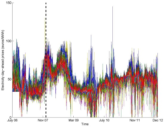
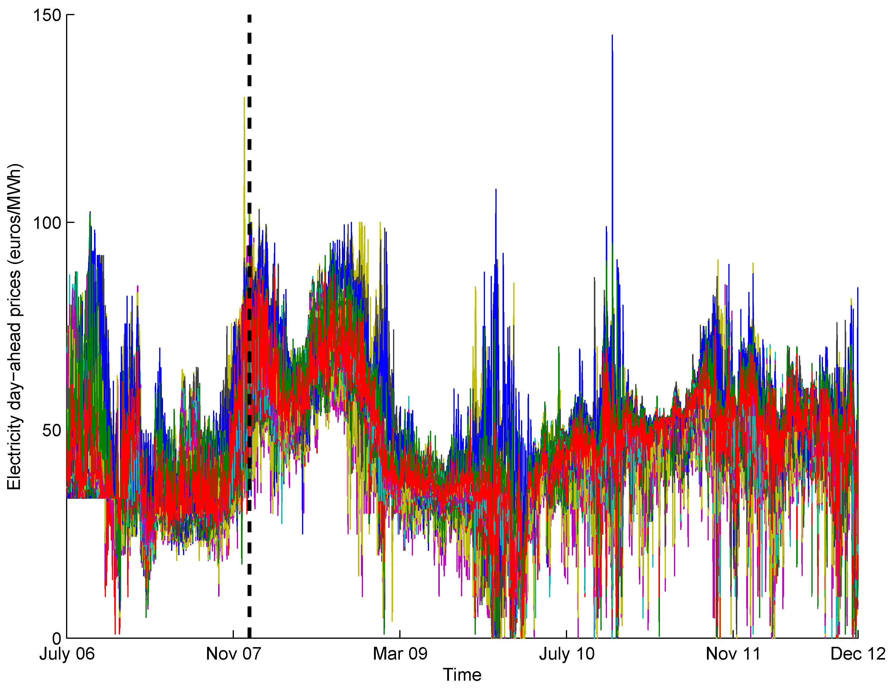
4.1. Data

We study a dataset of spot prices for the Iberian (Spain and Portugal) electricity market from July 2006 to December 2012. The dataset is presented in Figure 1. There is a common pattern in the evolution of the hourly series. The period before 2008 (Figure 1 to the left of the dashed line) is only used as historical data; the first predicted day is 1 January 2008 and the last one 31 December 2012.

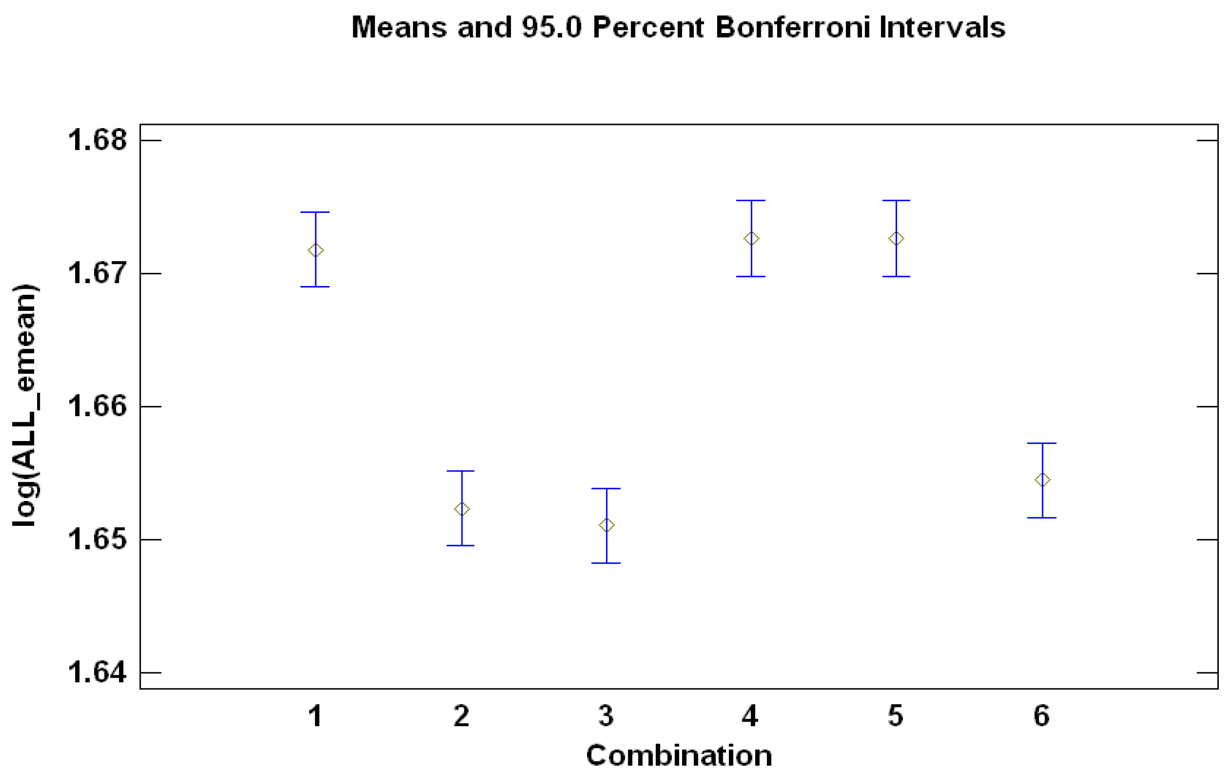
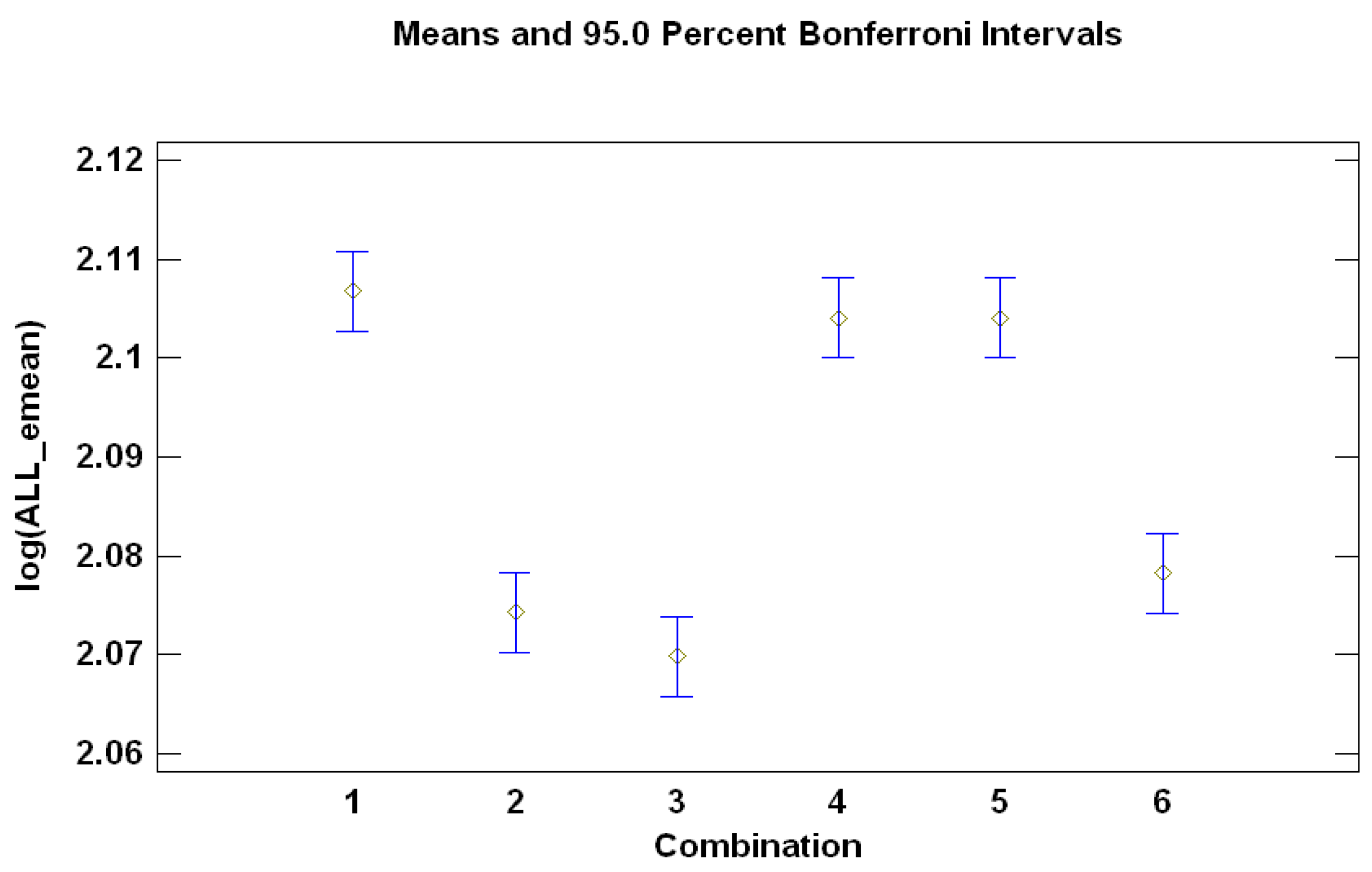
4.2. ANOVA for a Comparison of Alternatives for Modeling

When modeling, some characteristics should be considered:

• Whether to use prices or the logarithm of prices (factor “LOG” or logarithm, with two levels, zero and one, when not taking logarithm or when doing so, respectively).
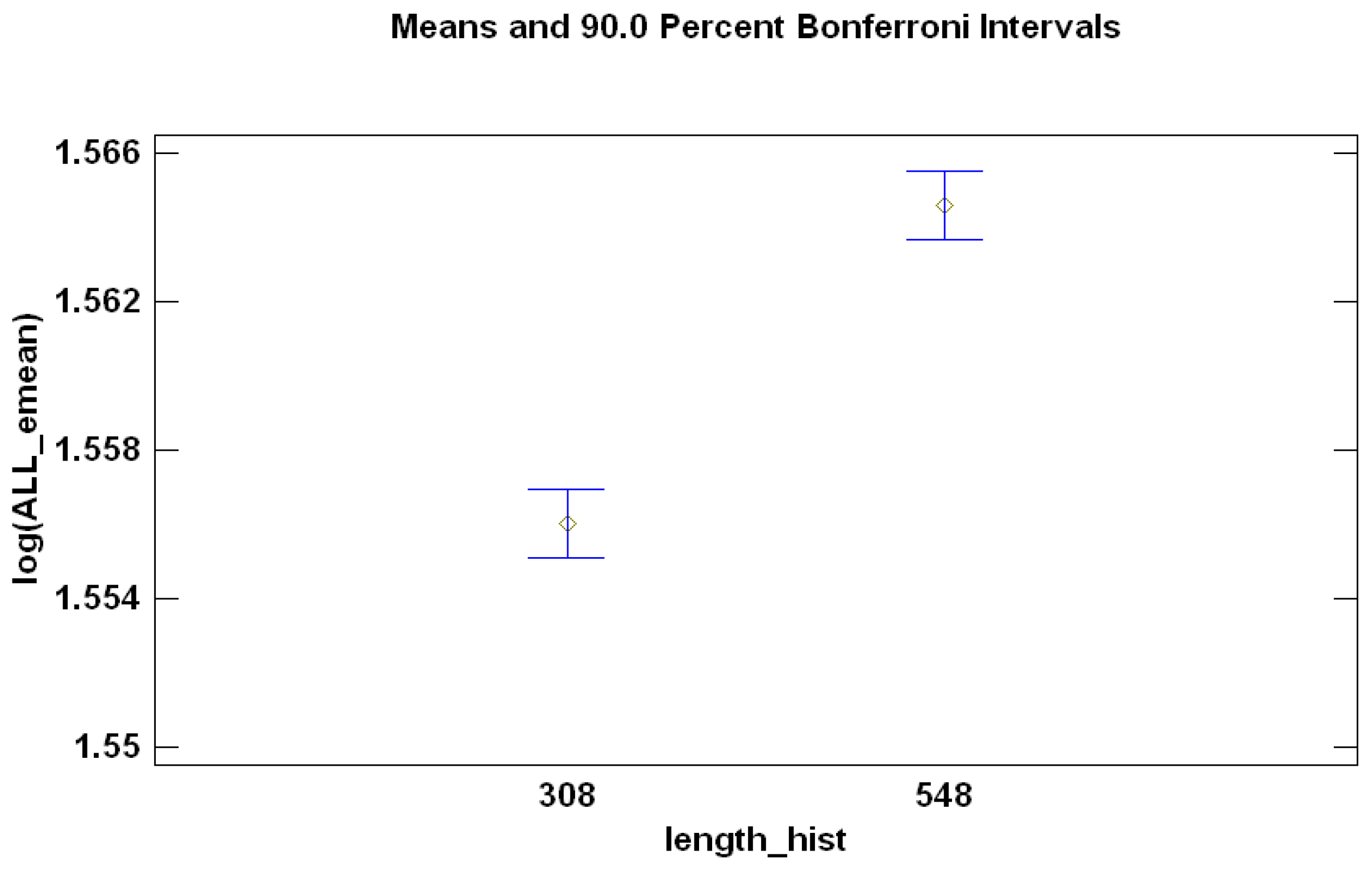
• The length of historical data for the rolling windows (44 weeks [12] or $1.5$ years).
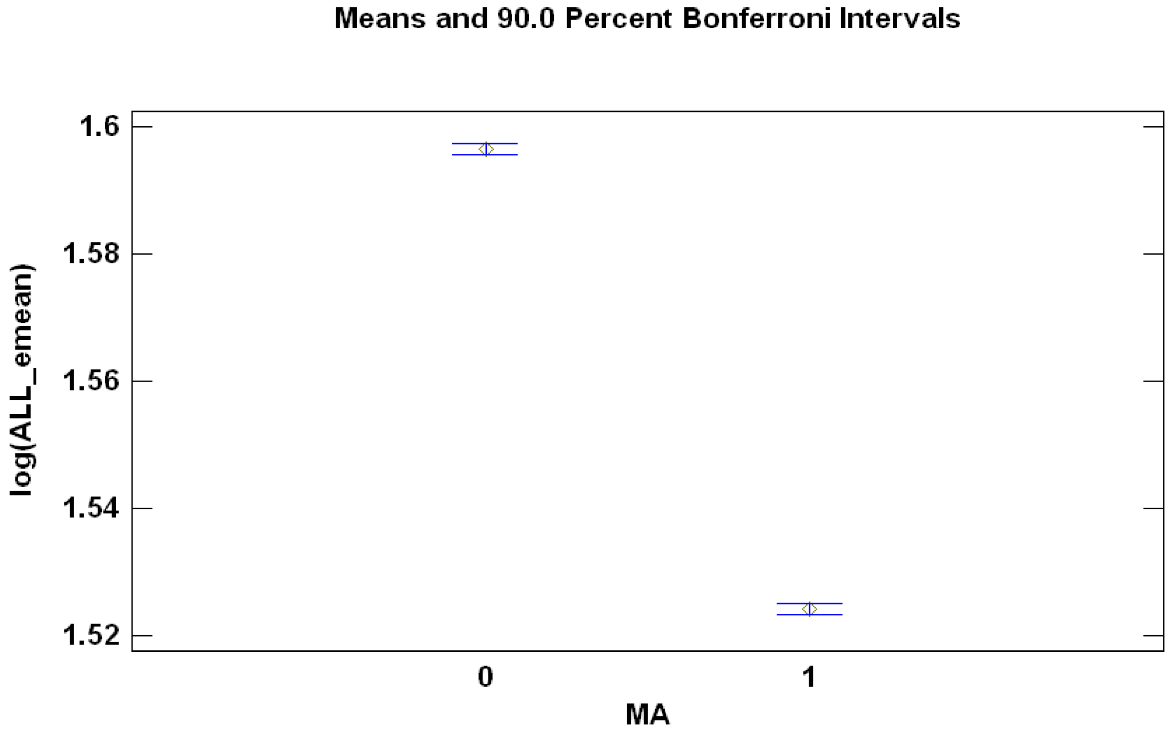
• Are common factors best fit by auto-regressive (AR) or auto-regressive-moving-average (ARMA)? The factor “MA” has two levels, zero (not including MA component) and one (including the MA component).
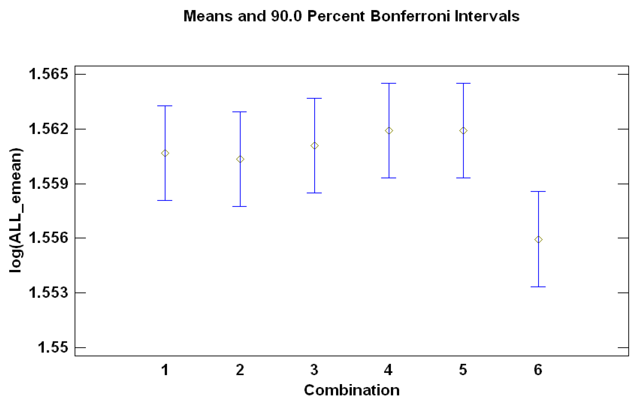
• Are there statistically-significant differences between the six possible forecasts combinations?

To compare these features, we have computed forecasts for every hour and day from 1 January 2008 until the end of 2012. This involves estimations for every hour of every day during five years, a long period that allows validating the results. There are $2\times 2\times 2\times 6=48$ cases resulting from combining all of the levels of the aforementioned factors (two values for LOG, two values for length, two values for MA and six combinations) that could affect the forecasting error. We analyze separately the results for different forecasting horizons: one-day-ahead (forecasting horizon $h=1$), one-week-ahead ($h=7$), one-month-ahead ($h=30$) and two-months-ahead ($h=60$).

Furthermore, and given the fact that forecasts have been computed for a large number of days, the particular ‘day’ could also explain some significant part of the variability of the response variable (in this case, the response variable is the accuracy metric MAE). For instance, if the prices in one day are rather unexpected (for being too low or high), the MAEs will be large, whatever historical length, combination of forecasts, logs or levels and using common factors with the MA component or not. This is the reason why the day is considered as a block in the computational experiment and the subsequent ANOVA performed. A complete reference on ANOVA and design of experiments is [42].

The equation of the model estimated (an ANOVA with four factors and one block (when including interactions, they were not significant, and the F-statistic is smaller than one, so they were removed from the model) for detecting which levels of the factors LOG, length, MA and combination previously described are preferred in terms of forecasting accuracy is the following:

$$\begin{array}{c}\hfill MA{E}_{ijkld}=\mu +{(\alpha )}_i+{(\beta )}_j+{(\gamma )}_k+{(\delta )}_l+{(ϵ)}_d+u_{ijkld}\end{array}$$

$$u_{ijkld}\sim NIID(0,{\sigma }_u^2)$$

(10)

where μ is the grand mean and ${(\alpha )}_i$, ${(\beta )}_i$, ${(\gamma )}_i$, ${(\delta )}_i$ and ${(ϵ)}_i$ are the main effects of the factors LOG, length, MA, combination and the block “day”, respectively. The main effect ${(\delta )}_l$ measures the increase/decrease of the average response of the combination of forecasts $l=1,2,3,4,5,6$ with respect to the average level; and similarly for the rest of the main effects. The noise term $u_{ijkld}$ includes all that is not explicitly taken into account in the model, but that somehow is able to explain some of the variability of the response variable $MA{E}_{ijkld}.$

Since we assume that the error term $u_{ijkld}$ is Gaussian, independently and identically distributed, with zero mean and variance ${\sigma }_u^2$, once the model has been estimated, a diagnostic check must be performed, testing that the $e_{ijkld}$ are homoskedastic, Gaussian and independent, where:

$$e_{ijkld}={\widehat{u}}_{ijkld}=MA{E}_{ijkld}-\widehat{\mu }-{(\widehat{\alpha })}_i-{(\widehat{\beta })}_j-{(\widehat{\gamma })}_k-{(\widehat{\delta })}_l-{(\widehat{ϵ})}_d$$

The results obtained for each forecast horizon are summarized and illustrated below. In all of the cases, the response variable was transformed after a first attempt to fit a model to the $MA{E}_{ijkld}$ because the residuals were heteroskedastic. The results shown hereafter consider the $\log (MA{E}_{ijkld})$ as the response variable. Given that the logarithm is a monotonically-increasing function, the results can be interpreted directly, and the best model corresponds to the smallest $\log (MA{E}_{ijkld})$, while the worst model to the largest $\log (MA{E}_{ijkld}).$

Summarizing the Conclusions from the ANOVAs

For all of the forecasting horizons considered, taking the logarithm of prices does not make a difference in performance. Regarding the length of the historic dataset, the shortest window is preferred for the forecasting horizons of one and seven-days-ahead (forecasts for the short term), while the long window of 1.5 years is preferred for the forecasting horizons of 30- and 60-days-ahead (long-term forecasts); this is consistent with the results in [5]. Furthermore, the MA terms for the factor models are statistically significant for all forecasting horizons, which means that modeling the common factors as ARMA reduces the error in comparison to modeling them as AR.

Regarding the combinations, the median-based combination, mean-based combination and mean BIC-based combination result in better forecasts than the benchmark BIC-selected model and the other combinations available for most forecasting horizons ($h=7$ onward). However, it is not clear that one of these three is always better: the confidence intervals for the median-based combination, mean-based combination and mean BIC-based combination usually overlap, indicating no significant difference between them.

For details of the results for each forecasting horizon, see the Appendix A.

4.3. Electricity Price Forecasting

In this section, the results of the forecast combinations are presented, in comparison with the best model selected with the BIC information criterion (this model may have one or two common factors, and each factor is modeled with an ARIMA model with parameters selected by BIC; the model is selected anew in each window) Forecasts are calculated for a long period, for each day and hour. The next paragraphs describe the technical details involved in estimation; Subsection 4.3.1 sheds light on the results involved in the estimation of each rolling window, and Subsection 4.3.2 presents the results for all days and hours.

Prices are transformed using logarithms to mitigate the existing heteroskedasticity, present in most commodity prices’ time series. Therefore, the series modeled are $y_t=log(P_t+k)$, where $P_t$ is the vector of 24 prices for day t, and $k=1000$ is a constant included to avoid a value of $log(0)$, which would happen when prices are equal to zero.

For medium- and long-term forecasting, forecasts of specific components are negligible. Therefore, we do not model these, but only the unobserved common factors, which explain the larger portion of the variability and capture the trend of the series in the long-run. This is consistent with the results in [5]. The prediction horizon will vary from 1 to 60 days, and once the factor(s) are modeled and predicted, the loading matrix is used to obtain the forecasts of the original 24-dimensional vector of prices. Then, the out-of-sample performance of the forecasts is evaluated.

We work with rolling windows of a length of 1.5 years (the best length for medium- and long-term forecasts according to the previous section); and estimate one and two common factors.

In each window, 36 alternative seasonal ARIMA$(p,d,q)\times (P,D,Q)s$ models ($p=1,2,3$, $d=0$, $q=1,2,3$, $P=0,1$, $D=1$, $Q=0,1$, $s=7$) are estimated for each factor. Weekly seasonality is included in the model ($s=7$), but yearly seasonality is not. This follows [5], who found no improvement in the prediction error when modeling yearly seasonality in the Iberian market, using a similar length of time for the estimation.

Therefore, there are 36 models that use only one factor, and 1296 models that use two factors; a total of 1332 different models, depending on how many factors they include and the parameters of the ARIMA$(p,d,q)\times (P,D,Q)s$ (in a total of 1767 time rolling windows). This makes it unfeasible to check the residuals behavior for each ARIMA model estimated (notwithstanding, TRAMO (the software employed to estimate the ARIMA models) calculates the p-value of the Ljung–Box statistic for each model and shows acceptable values for most cases). However, three of the five forecast combinations under consideration are based on BIC, so “badly”-behaved models (poor fit will be associated with a high residuals variance) will be assigned small or negligible weights in the final forecast. Furthermore, the median-based combination is not affected by outliers due to “badly”-behaved models. Only the mean combination may be affected by them, but based on

Table 1. Weekly, monthly and bi-monthly MAE and median absolute error (MedAE) for the Iberian market for the period 1 January 2008–31 December 2012.

	BIC-Selected	Median-Based	Mean-Based	BIC-Based	BIC 50%	Mean BIC-Based
	Model	Combination	Combination	Combination	Combination	Combination
Weekly
MAE	5.9455	5.8690	5.8965	5.9384	5.9384	5.8397
MedAE	5.3515	5.2433	5.2677	5.3444	5.3444	5.2275
Monthly
MAE	6.9069	6.6952	6.7097	6.8934	6.8934	6.6526
MedAE	6.3635	6.1179	6.1367	6.3484	6.3484	6.0882
Bi-Monthly
MAE	7.8184	7.5456	7.5512	7.8014	7.8014	7.4867
MedAE	7.3047	7.0081	7.0157	7.2844	7.2844	6.9539

, median and mean combinations reveal similar results. If there were fewer models or the analysis were limited to a shorter period, residual checking could be performed before forecast averaging. In this case, it would be reasonable to obtain slightly better results.

Notwithstanding the large number of models, the estimation for each individual window of time takes only a few minutes; therefore, the procedure could be used in real time. Furthermore, even though with such a large number of models, some will be superfluous, the combinations that use weights depending on the BIC will assign them nearly null weights.

4.3.1. Illustration for a Single Forecasting Window

Before proceeding with the presentation of the results, this subsection is used to gain insight into the role of the common factors, as well as the forecasting combinations. With this aim, the estimation for one window of the dataset is analyzed in further detail.

The role of the underlying factors is hereby clarified. Considering as an example the first rolling window in the estimation, Figure 2 presents the first and second common factors, as well as the weights assigned to them for each of the 24 h. For the first factor, which explains 64.6% of the data variability, weights are heavy from Hours 8–24, when most people are awake. Then, it is possible to interpret that this factor mainly records the general behavior of prices during hours when people are awake. On the other hand, the weights of the second factor are positive from 9–18 and negative otherwise. This coincides with usual working hours (or, alternatively, sunlight hours). Therefore, the second factor, which accounts for 13.8% of the data variability, would capture changes in the price relation of working vs. non-working hours. Notice that some models would include only the first factor, while others will include the first and second common factors. Models with more factors have been excluded from the analysis (setting $r\le 2$) because already around 80% of the data variability is explained by two factors, and it should be noted that there is a computational burden of incorporating an additional factor.

The massive estimations performed make it unfeasible to provide the estimation results for each of the 1336 models and for each of the 1767 rolling windows of time. However, as an illustration, for the first rolling window, taking for example the first factor and the ARIMA model of order $p=1$, $q=1$, $P=0$, $Q=0$, the coefficients would be the following: $\varphi =0.7145$, $\theta =-0.1319$ (both significant).

To shed some light on how the alternative models enter the combinations, Figure 3 presents the BIC values for the 1332 previously-mentioned models. For illustrative purposes, also the first rolling window of the data is employed. The horizontal axis corresponds to the indexes of the models. The first 36 values (X axis 1–36) represent models with only one factor ($r=1$), starting with parameters $p=1$, $q=1$, $P=0$, $Q=0$ for X axis = 1, then $p=1$, $q=1$, $P=0$, $Q=1$ for X axis = 2, until $p=3$, $q=3$, $P=1$, $Q=1$ for X axis = 36. X axis 37–1336 correspond to models with two factors ($r=2$). In X axis = 1336, the order of the ARIMA models for the two factors coincide, $p=3$, $q=3$, $P=1$, $Q=1$. For BIC-dependent combinations, the smaller the BIC value, the greater that model’s weight. In this way, better performing models are rewarded. It is clear that there are some models with predominant low BIC (i.e., high weights). Of course, if all considered models had a poor goodness of fit, then it would be reasonable that the combinations would inherit that bad performance. The claim in this work is that those combinations would be, at least, as good as the best considered model.

4.3.2. Forecasting Results

In Table 1, the MAE and MedAE for the BIC-selected model and for the alternative combinations are presented for weekly, monthly and bi-monthly forecasts. The same exercise was performed employing the root mean squared error (see [40] for an explanation of how to calculate this measure of the error) and similar results were obtained.

In conclusion, there is an improvement in prediction when using forecast combinations, in comparison with the best model selected according to the BIC criterion. In this case, the improvement of the mean-based forecast combinations is clear, while for the BIC-based combination, the improvement in the forecasting errors is smaller. Even though the decrease in the errors is small when we compare the benchmark to the combinations, it is steady, supporting the conclusion obtained in the ANOVA in which some combinations are statistically significantly better than the benchmark.

As an illustration of long-run performance, we also obtained forecasts for up to one-year-ahead, considering the period to forecast between 1 January 2012 and 30 December 2012 (2012 is a leap year). In this case, the annual MAE and MedAE (values comparable to Table 1) are 8.0669 and 7.2699, respectively, for the best combination for the one-year-ahead horizon: the mean-based combination. Even though the mean-based combination presents the smallest errors for the annualized forecast, it has greater volatility than the BIC-based combination. A similar situation is recorded for the rest of the combinations in comparison to the BIC-based one.

Furthermore, there is practically no deterioration of these long-run forecasts with respect to shorter forecast horizons.

Table 2. MAE and MedAE for the Iberian market: predictions for 2012.

		BIC-Selected	Median-Based	Mean-Based	BIC-Based	BIC 50%	Mean BIC-Based
		Model	Combination	Combination	Combination	Combination	Combination
January	MAE	5.9914	6.7577	6.8780	6.0130	6.0130	6.4687
2012	MedAE	5.3622	6.4678	6.7260	5.2593	5.2593	6.0601
February	MAE	6.4675	7.2435	7.4060	6.4906	6.4906	6.9594
2012	MedAE	6.5416	7.4396	7.5021	6.6464	6.6464	7.2376
March	MAE	6.9734	6.1102	6.0922	6.8243	6.8243	6.1867
2012	MedAE	6.0546	5.3264	5.256	6.0065	6.0065	5.2017
April	MAE	13.5490	12.4104	12.2801	13.3762	13.3762	12.5287
2012	MedAE	13.2217	10.7761	10.0235	13.1850	13.1850	11.2624
May	MAE	10.8668	9.3332	9.1965	10.6543	10.6543	9.5498
2012	MedAE	9.3751	7.5543	7.4841	9.1088	9.1088	7.7359
June	MAE	6.0767	6.3919	6.6578	6.1280	6.1280	6.2612
2012	MedAE	5.5188	5.8455	6.3053	5.5588	5.5588	5.8795
July	MAE	5.9894	5.5998	5.7148	5.9188	5.9188	5.5693
2012	MedAE	5.8066	5.6251	5.7086	5.8096	5.8096	5.4504
August	MAE	6.3186	5.6453	5.7619	6.2278	6.2278	5.7026
2012	MedAE	5.9970	5.4338	5.6871	5.8635	5.8635	5.0984
September	MAE	8.1682	7.4471	7.4487	8.0259	8.0259	7.4593
2012	MedAE	6.9071	6.3828	6.9140	6.8746	6.8746	6.3112
October	MAE	9.1325	7.9165	7.8303	8.9732	8.9732	8.1128
2012	MedAE	6.6286	6.2065	6.4013	6.4605	6.4605	5.3778
November	MAE	11.4100	9.7935	9.5407	11.1893	11.1893	10.1087
2012	MedAE	9.2314	6.9678	6.3402	9.1100	9.1100	7.6911
December	MAE	13.1200	12.2841	12.1081	12.9827	12.9827	12.3144
2012	MedAE	9.3700	9.9895	9.2326	9.7346	9.7346	9.7757

supports this conclusion. In this table, the values of the MAE and MedAE for each month of 2012 are presented for the benchmark and the alternative combinations. When taking into account the average of each month, the mean-based combination is the best performer (presents the smallest errors most months), followed by the mean-BIC combination. This performance is better in the medium and long run than in the short term: for the first two months, the BIC-selected model provides a smaller error. Similarly, [28] obtain that the relative performance of the combinations in comparison to the best model improve as the forecasting horizon is extended. All in all, the mean-based combination is competitive when compared to other combinations, a conclusion also supported by [18].

5. Conclusions and Further Lines of Research

In this paper, dynamic factor models and forecast combination techniques have been jointly employed to obtain predictions of spot market electricity prices in the Iberian market. The main contribution consists, therefore, of combining two streams of literature in order to obtain forecasts that outperform those resulting from the individual models. In this respect, there are three combinations that clearly outperform the benchmark: the median-based combination, the mean-based combination and the mean BIC-based combination. This conclusion is supported by the ANOVA of the combinations for forecast horizons one-day-ahead, seven-days-ahead, 30-days-ahead and 60-days-ahead. For the extended prediction (up to one-year-ahead, taking the case of the year 2012), the results point out that the benefit of forecast combinations is greater for the medium/large forecast horizon than for the short term.

In the process of trying to obtain the best possible results, different aspects of the available models were compared. In this regard, the main conclusions are that longer historic datasets benefit longer forecasting horizons, and the error is reduced by the inclusion of MA terms when modeling the unobserved factors (vs. AR models).

This application reflects how the methodology works for a current dataset. The numerical results for electricity prices, which is a difficult to predict series, are good. An effort has been made to obtain the results for many time horizons ($h=1$ to $h=60$), for every day and hour for 1 January 2008–31 December 2012 and considering several models for the factors, enhancing the validity of our proposal. In other words, forecasts are obtained for the very short (one day) and short term (a few days ahead), like most of other works, as well as for the medium term, which is an extension not customary in the literature. As previously explained, this approach can be employed to obtain long-term forecasts (even up to a year) not experiencing a degradation of accuracy, which is a drawback that most applications suffer from.

Numerous lines of research remain open in relation to this topic. For instance, in this work, few techniques for combining forecasts are employed besides the mean, and weights depend on the overall performance of the particular model to be used in the combination in terms of the BIC information criterion. However, there are several other, Bayesian and classical techniques to determine such weights. In particular, it would be interesting to compare the performance of both types of techniques. Furthermore, in this article, we have mostly worked with fixed weights; however, these could change in a predefined way for different forecasting horizons. Furthermore, weights could be adaptive to the performance of the models (as in [16]).

The use of ARIMA models for the common factors allows one to maintain the number of parameters to estimate low, but it may also signify a constraint in the improvement that can be achieved from the combinations of forecasts. A future line of work is including other models for the factors, such as the SeaDFA of [5] (when employing the SeaDFA formulation, it is assumed that $F_t$ follows a VARIMA model) or the Generalized AutoRegressive Conditionally Heteroscedastic (GARCH)-SeaDFA.

It is also left for future work to incorporate in the forecast combination other forecasting methods (not necessarily involving DFM); for example, the predictions obtained by the mixed model in [4], which presents extremely accurate short-term predictions for the Iberian market. With weights evolving for different time-horizons, including this model for short-term predictions could improve the results.

A further improvement could consist of employing explanatory variables that drive spot prices in the models. Some examples of these variables are demand, weather conditions, fuel prices, production by technology and excess capacity. Interesting references are [21,41]. However, for this, it would be necessary to assess if the uncertainty in the prediction of the explanatory variables does not outweigh the improvement in the forecast of the price. In a similar line of research, regime switching models could be employed to deal with spikes in the price series.

Last, bootstrap procedures could be used to obtain confidence intervals of the predictions and, in this way, assess the uncertainty involved in the forecasts.

References

- Weron, R. Electricity price forecasting: A review of the state-of-the-art with a look into the future. Int. J. Forecast. 2014, 30, 1030–1081. [Google Scholar] [CrossRef]
- Huisman, R.; Huurman, C.; Mahieu, R. Hourly electricity prices in day-ahead markets. Energy Econ. 2007, 29, 240–248. [Google Scholar] [CrossRef]
- Panagiotelis, A.; Smith, M. Bayesian Density Forecasting of intraday electricity prices using multivariate skewed t distributions. Int. J. Forecast. 2008, 24, 710–727. [Google Scholar] [CrossRef]
- García-Martos, C.; Rodríguez, J.; Sánchez, M. Mixed Models for Short-Run Forecasting of Electricity Prices: Application for the Spanish Market. IEEE Trans. Power Syst. 2007, 22, 544–552. [Google Scholar] [CrossRef]
- Alonso, A.; García-Martos, C.; Rodríguez, J.; Sánchez, M. Seasonal Dynamic Factor Analysis and Bootstrap Inference: Application to Electricity Market Forecasting. Technometrics 2011, 53, 137–151. [Google Scholar] [CrossRef]
- Sargent, T.; Sims, C. Business Cycle Modelling Without Pretending to Have Too Much a Priori Economic Theory, New Methods in Business Cycle Research; Federal Reserve Bank of Minneapolis: Minneapolis, MN, USA, 1977; Volume 55. [Google Scholar]
- Geweke, J. The Dynamic Factor Analysis of Economic Time Series. Latent Variables in Socio-Economic Models; North-Holland: Amsterdam, The Netherlands, 1977. [Google Scholar]
- Lee, R.; Carter, L. Modelling and forecasting U.S. mortality. J. Am. Stat. Assoc. 1992, 87, 659–671. [Google Scholar]
- Stock, J.; Watson, M. Forecasting using principal components from a large number of predictors. J. Am. Stat. Assoc. 2002, 97, 1167–1179. [Google Scholar] [CrossRef]
- Peña, D.; Poncela, P. Forecasting with Nonstationary Dynamic Factor Models. J. Econom. 2004, 119, 291–321. [Google Scholar] [CrossRef]
- Peña, D.; Poncela, P. Nonstationary dynamic factor analysis. J. Stat. Plan. Inference 2006, 136, 1237–1257. [Google Scholar] [CrossRef]
- García-Martos, C.; Rodríguez, J.; Sánchez, M. Forecasting electricity prices by extracting dynamic common factors: Application to the Iberian market. IET Gener. Transm. Distrib. 2012, 6, 11–20. [Google Scholar] [CrossRef]
- Peña, D.; Box, G. Identifying a simplifying structure in time series. J. Am. Stat. Assoc. 1987, 82, 836–843. [Google Scholar] [CrossRef]
- Maciejowska, K.; Weron, R. Forecasting of daily electricity prices with factor models: Utilizing intra-day and inter-zone relationships. Comput. Stat. 2015, 30, 805–819. [Google Scholar] [CrossRef]
- Clemen, R. Combining forecasts: A review and annotated bibliography. Int. J. Forecast. 1989, 5, 559–583. [Google Scholar] [CrossRef]
- Sánchez, I. Short-term prediction of wind energy production. Int. J. Forecast. 2006, 22, 43–56. [Google Scholar] [CrossRef]
- Bjørnland, H.; Gerdrup, K.; Jore, A.; Smith, C.; Thorsrud, L. Does forecast combination improve Norges Bank inflation forecasts? Oxford Bull. Econ. Stat. 2012, 74, 163–179. [Google Scholar] [CrossRef]
- Bordignon, S.; Bunn, D.; Lisi, F.; Nan, F. Combining day-ahead forecasts for British electricity prices. Energy Econ. 2013, 35, 88–103. [Google Scholar] [CrossRef]
- Nowotarskia, J.; Raviv, E.; Trückc, S.; Werona, R. An empirical comparison of alternate schemes for combining electricity spot price forecasts. Energy Econ. 2014, 46, 395–412. [Google Scholar] [CrossRef]
- Raviv, E.; Bouwman, K.; Van Dijk, D. Forecasting day-ahead electricity prices: Utilizing hourly prices. Energy Econ. 2015, 50, 227–239. [Google Scholar] [CrossRef]
- Monteiro, C.; Fernandez-Jimenez, L.; Ramirez-Rosado, I. Explanatory Information Analysis for Day-Ahead Price Forecasting in the Iberian Electricity Market. Energies 2015, 8, 10464–10486. [Google Scholar] [CrossRef]
- García-Martos, C.; Caro, E.; Sánchez, M. Electricity price forecasting accounting for renewable energies: Optimal combined forecasts. J. Oper. Res. Soc. 2015, 66, 871–884. [Google Scholar] [CrossRef]
- Poncela, P.; Rodriguez, J.; Sánchez-Mangas, R.; Senra, E. Forecast combination through dimension reduction techniques. J. Forecast. 2011, 27, 224–237. [Google Scholar] [CrossRef]
- Kuzin, V.; Marcellino, M.; Schumacher, C. Pooling versus model selection for nowcasting GDP with many predictors: Empirical evidence for six industrialized countries. J. Appl. Econom. 2012, 28, 32–411. [Google Scholar] [CrossRef]
- Martínez-Álvarez, F.; Troncoso, A.; Asencio-Cortés, G.; Riquelme, J. A Survey on Data Mining Techniques Applied to Electricity-Related Time Series Forecasting. Energies 2015, 8, 13162–13193. [Google Scholar] [CrossRef]
- Stock, J.; Watson, M. Combination forecasts of output growth in a seven country dataset. J. Forecast. 2004, 23, 405–430. [Google Scholar] [CrossRef]
- Yang, Y. Combining forecasting procedures: some theoretical results. Econom. Theory 2004, 20, 176–222. [Google Scholar] [CrossRef]
- Elliott, G.; Granger, C.; Timmermann, A. Handbook of Economic Forecasting; North-Holland: Oxford, UK, 2006; Volume 1. [Google Scholar]
- Swanson, N.; Zeng, T. Choosing Among Competing Econometric Forecasts: Regression-Based Forecast Combination Using Model Selection. J. Forecast. 2001, 20, 425–440. [Google Scholar] [CrossRef]
- Schwarz, G. Estimating the dimension of a model. Ann. Stat. 1978, 6, 461–464. [Google Scholar] [CrossRef]
- Wright, J. Bayesian Model Averaging and exchange rate forecasts. J. Econom. 2008, 146, 329–341. [Google Scholar] [CrossRef]
- Leamer, E. Specification Searches: Ad Hoc Inference with Nonexperimental Data; John Wiley & Sons: New York, NY, USA, 1978. [Google Scholar]
- Raftery, A. Bayesian Model Selection in Social Research. Sociol. Methodol. 1995, 25, 111–163. [Google Scholar] [CrossRef]
- Raftery, A.; Madigan, D.; Hoeting, J. Bayesian model averaging for linear regression models. J. Am. Stat. Assoc. 1997, 92, 179–191. [Google Scholar] [CrossRef]
- Chipman, H.; George, E.; McCulloch, R. The practical implementation of Bayesian model selection. IMS Lect. Notes 2001, 38, 70–134. [Google Scholar]
- Koop, G.; Potter, S. Forecasting in Large Macroeconomic Panels Using Bayesian Model Averaging; Federal Reserve Bank of New York: New York, NY, USA, 2003; Volume 163. [Google Scholar]
- Cremers, K. Stock return predictability: A Bayesian model selection perspective. Rev. Financ. Stud. 2002, 15, 1223–1249. [Google Scholar] [CrossRef]
- Billio, M.; Casarin, R.; Ravazzolo, F.; Van Dijk, H. Combining Predictive Densities using Nonlinear Filtering with Applications to US Economics Data. Tinbergen Institute Discussion Paper. 2011. Available online: http://papers.ssrn.com/sol3/papers.cfm?abstract_id=1967435 (accessed on 18 July 2016).
- Conejo, A.; Contreras, J.; Espínola, R.; Plazas, M. Forecasting electricity prices for a day-ahead poll-based electric energy market. Int. J. Forecast. 2005, 21, 435–462. [Google Scholar] [CrossRef]
- Hyndman, R.; Koehler, A. Another look at measures of accuracy. Int. J. Forecast. 2006, 22, 679–688. [Google Scholar] [CrossRef]
- Bello, A.; Reneses, J.; Muñoz, A. Medium-Term Probabilistic Forecasting of Extremely Low Prices in Electricity Markets: Application to the Spanish Case. Energies 2016, 9, 193–219. [Google Scholar] [CrossRef]
- Montgomery, D.C. Design and Analysis of Experiments; Wiley: New York, NY, USA, 1984. [Google Scholar]