
Statistical Analysis of Wave Climate Data Using Mixed Distributions and Extreme Wave Prediction


Abstract
:1. Introduction
2. Statistical Analysis of Measured Wave Data
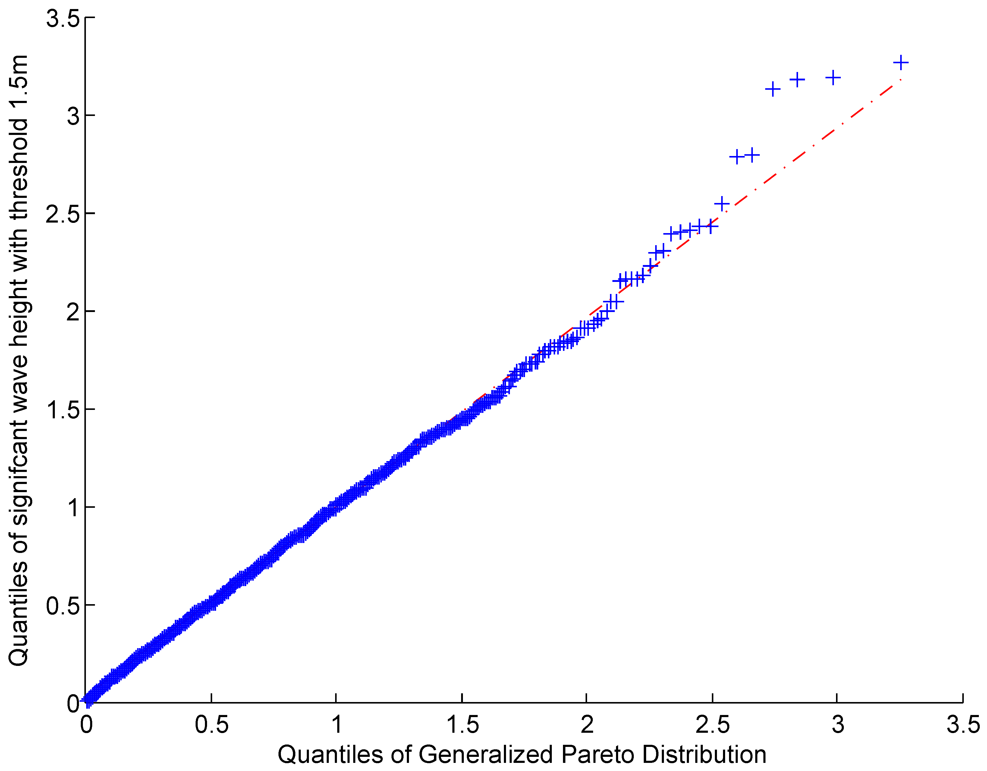
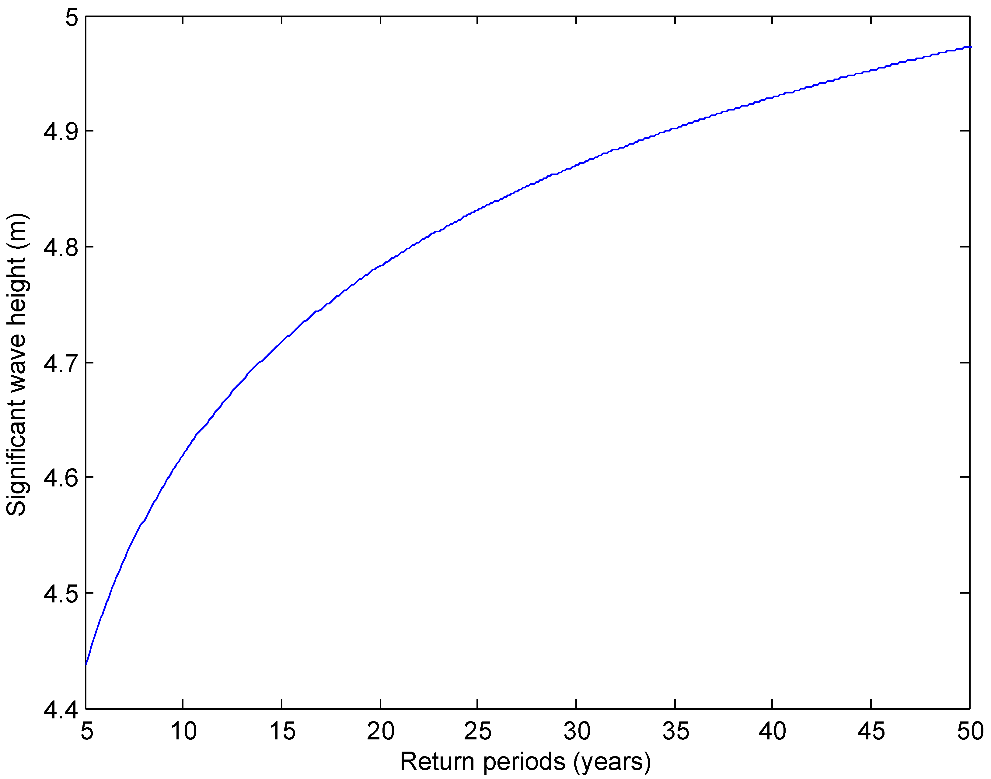
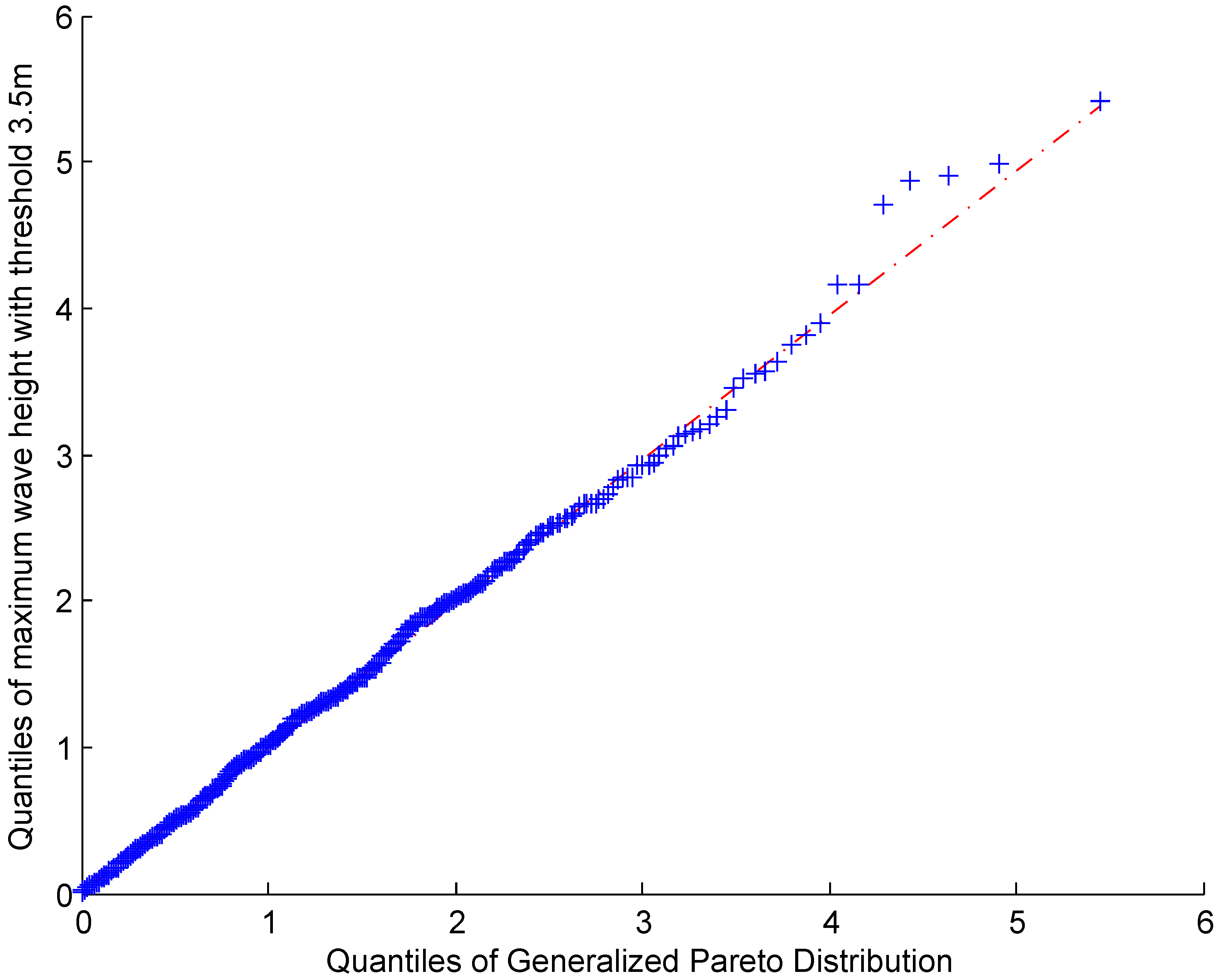
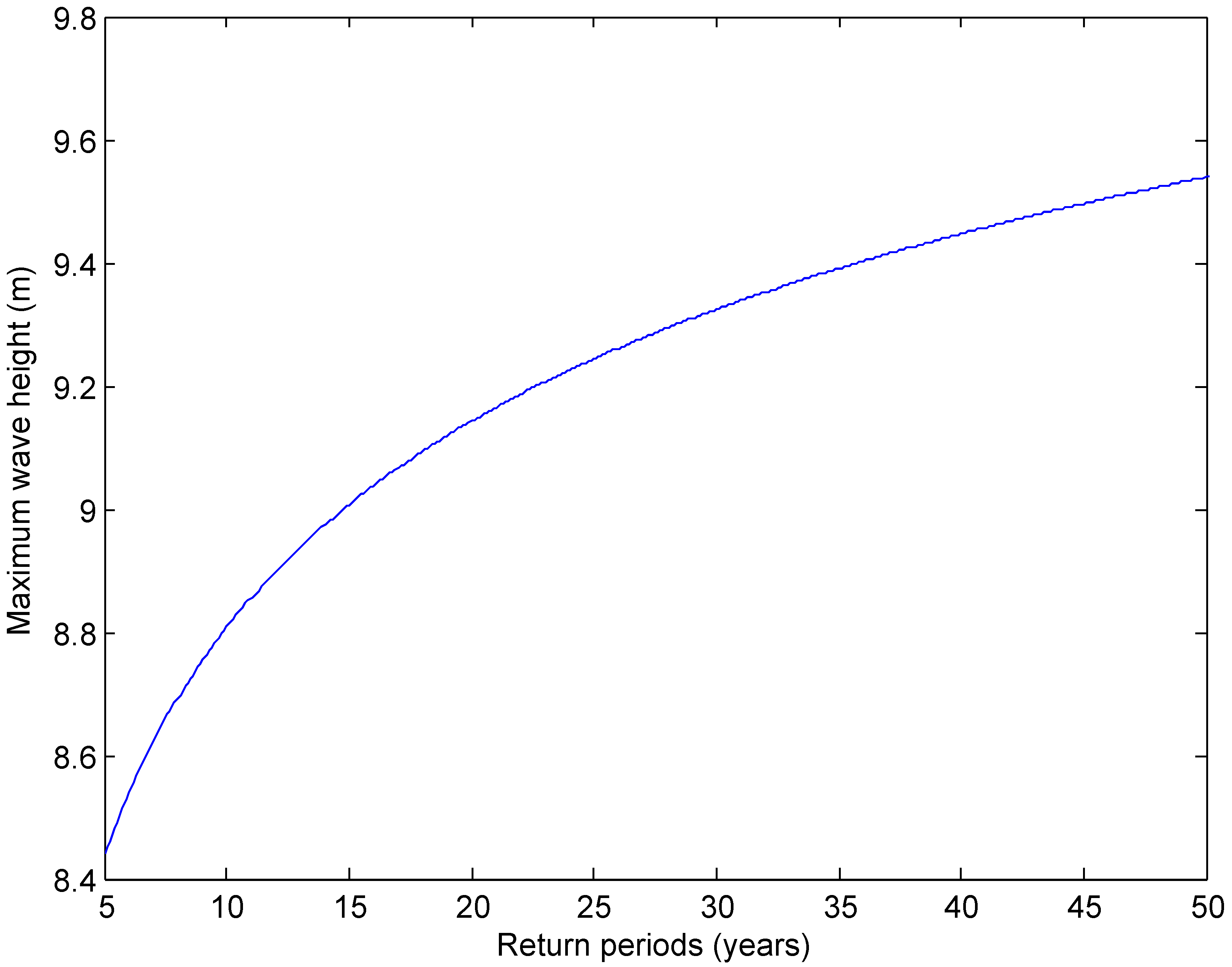
3. Extreme Wave Estimation
4. Wave Height Distribution Modelling
4.1. Mixed-Distribution Model
4.2. Application of the Mixed-Distribution Model to Different Measured Wave Data
5. Conclusions
Acknowledgments
Author Contributions
Conflicts of Interest
References
- 2013 Annual Report; The Executive Committee of Ocean Energy Systems Implementing Agreement on Ocean Energy Systems (IEA-OES): Lisbon, Portugal, 2013.
- Groll, N.; Grabemann, I.; Gaslikova, L. North Sea wave conditions: An analysis of four transient future climate realizations. Ocean Dyn. 2013, 64, 1–12. [Google Scholar] [CrossRef]
- Carillo, A.; Liberti, L.; Sannino, G. Present climate wave energy potential along the Western Sardinia coast (Italy). In Proceedings of the 2013 IEEE International Conference on Clean Electrical Power (ICCEP), Alghero, Italy, 11–13 June 2013; pp. 209–212.
- Duclos, G.; Babarit, A.; Clément, A.H. Optimizing the Power Take Off of a Wave Energy Converter With Regard to the Wave Climate. J. Offshore Mech. Arct. Eng. 2006, 128, 56–64. [Google Scholar] [CrossRef]
- Leijon, M.; Boström, C.; Danielsson, O.; Gustafsson, S.; Haikonen, K.; Langhamer, O.; Strömstedt, E.; Stålberg, M.; Sundberg, J.; Svensson, O.; et al. Wave Energy from the North Sea: Experiences from the Lysekil Research Site. Surv. Geophys. 2008, 29, 221–240. [Google Scholar] [CrossRef]
- Hong, Y.; Hultman, E.; Castellucci, V.; Ekergård, B.; Sjökvist, L.; Elamalayil Soman, D.; Krishna, R.; Haikonen, K.; Baudoin, A.; Lindblad, L.; et al. Status Update of the Wave Energy Research at Uppsala University. In Proceedings of the 10th European Wave and Tidal Energy Conference (EWTEC), Aalborg, Denmark, 2–5 September 2013.
- Parwal, A.; Remouit, F.; Hong, Y.; Francisco, F.; Castellucci, V.; Hai, L.; Ulvgård, L.; Li, W.; Lejerskog, E.; Baudoin, A. Wave Energy Research at Uppsala University and the Lysekil Research Site, Sweden: A Status Update. In Proceedings of the 11th European Wave and Tidal Energy Conference, Nantes, France, 6–11 September 2015.
- Soares, C.G.; Scotto, M. Modelling uncertainty in long-term predictions of significant wave height. Ocean Eng. 2001, 28, 329–342. [Google Scholar] [CrossRef]
- Muraleedharan, G.; Lucas, C.; Soares, C.G.; Unnikrishnan Nair, N.; Kurup, P.G. Modelling significant wave height distributions with quantile functions for estimation of extreme wave heights. Ocean Eng. 2012, 54, 119–131. [Google Scholar] [CrossRef]
- Ferreira, J.A.; Soares, C.G. Modelling the long-term distribution of significant wave height with the Beta and Gamma models. Ocean Eng. 1999, 26, 713–725. [Google Scholar] [CrossRef]
- Kim, S.U.; Kim, G.; Jeong, W.M.; Jun, K. Uncertainty analysis on extreme value analysis of significant wave height at eastern coast of Korea. Appl. Ocean Res. 2013, 41, 19–27. [Google Scholar] [CrossRef]
- Prevosto, M.; Krogstad, H.E.; Robin, A. Probability distributions for maximum wave and crest heights. Coast. Eng. 2000, 40, 329–360. [Google Scholar] [CrossRef]
- Ferreira, J.A.; Soares, C.G. Modelling distributions of significant wave height. Coast. Eng. 2000, 40, 361–374. [Google Scholar] [CrossRef]
- Muraleedharan, G.; Rao, A.D.; Kurup, P.G.; Nair, N.U.; Sinha, M. Modified Weibull distribution for maximum and significant wave height simulation and prediction. Coast. Eng. 2007, 54, 630–638. [Google Scholar] [CrossRef]
- Soares, C.G.; Ferreira, A.M.; Cunha, C. Linear models of the time series of significant wave height on the Southwest Coast of Portugal. Coast. Eng. 1996, 29, 149–167. [Google Scholar] [CrossRef]
- Kim, C.H. Nonlinear Waves and Offshore Structures, 1st ed.; World Scientific Publishing Company: Hackensack, NJ, USA, 2008; pp. 12–53. [Google Scholar]
- Guide to Wave Analysis and Forecasting; World Meteorological Organization (WMO): Geneva, Switzerland, 1998; Volume 1998, pp. 101–119.
- Pastor, J.; Liu, Y.; Dou, Y. Wave Energy Resource Analysis for Use in Wave Energy Conversion. In Proceedings of the Industrial Energy Technology Conference, New Orleans, LA, USA, 20–23 May 2014.
- Guiberteau, K.L.; Liu, Y.; Lee, J.; Kozman, T.A. Investigation of Developing Wave Energy Technology in the Gulf of Mexico. Distrib. Gener. Altern. Energy J. 2012, 27, 36–52. [Google Scholar] [CrossRef]
- Mathiesen, M.; Goda, Y.; Hawkes, P.J.; Mansard, E.; Martín, M.J.; Peltier, E.; Thompson, E.F.; Van Vledder, G. Recommended practice for extreme wave analysis. J. Hydraul. Res. 1994, 32, 803–814. [Google Scholar] [CrossRef]
- Fang, Z.; Dai, S.; Jin, C. On the long-term joint distribution of characteristic wave height and period and its application. Acta Oceanol. Sin. 1989, 8, 315–325. [Google Scholar]
- Mazas, F.; Hamm, L. A multi-distribution approach to POT methods for determining extreme wave heights. Coast. Eng. 2011, 58, 385–394. [Google Scholar] [CrossRef]
- Waters, R.; Engström, J.; Isberg, J.; Leijon, M. Wave climate off the Swedish west coast. Renew. Energy 2009, 34, 1600–1606. [Google Scholar] [CrossRef]
- Ashkar, F.; Tatsambon, C.N. Revisiting some estimation methods for the generalized Pareto distribution. J. Hydrol. 2007, 346, 136–143. [Google Scholar] [CrossRef]
- Holthuijsen, L.H. Waves in Oceanic and Coastal Waters; Cambridge University Press: Cambridge, UK, 2007; pp. 74–105. [Google Scholar]
- De Zea Bermudez, P.; Kotz, S. Parameter estimation of the generalized Pareto distribution—Part I. J. Stat. Plan. Inference 2010, 140, 1353–1373. [Google Scholar] [CrossRef]
- Pickands, J., III. Statistical Inference Using Extreme Order Statistics. Ann. Stat. 1975, 3, 119–131. [Google Scholar]
- Ferreira, J.A.; Soares, C.G. An Application of the Peaks over Threshold Method to Predict Extremes of Significant Wave Height. J. Offshore Mech. Arct. Eng. 1998, 120, 165. [Google Scholar] [CrossRef]
- Smith, E.P. An Introduction to Statistical Modeling of Extreme Values. Technometrics 2002, 44, 397. [Google Scholar] [CrossRef]


| Return Period | 25 Years | 50 Years |
|---|---|---|
| Significant wave height | 4.83 m | 4.96 m |
| Maximum wave height | 9.24 m | 9.52 m |
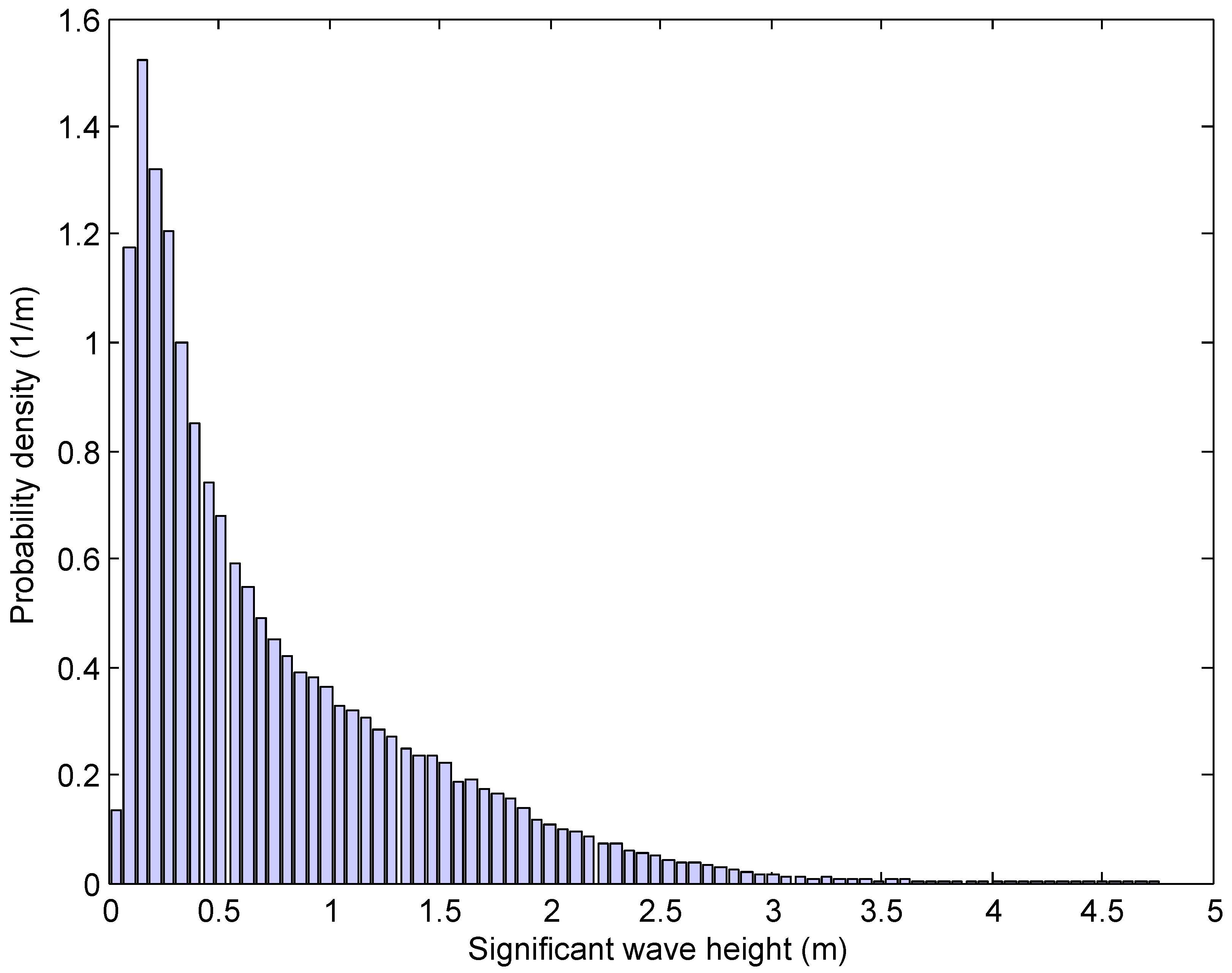
| Distribution | Parameters | R-Square | Root Mean Squared Error |
|---|---|---|---|
| Rayleigh | 0.703 | 0.382 | 0.248 |
| Weibull | 0.801, 1.198 | 0.914 | 0.093 |
| Lognormal | −0.682, 0.946 | 0.968 | 0.056 |
| Distribution | Parameters | Weights | R-Square | Root Mean Squared Error |
|---|---|---|---|---|
| Lognormal-Rayleigh | −1.190, 0.755 0.994 | 0.585 0.415 | 0.994 | 0.025 |
| Lognormal-Weibull | −1.461, 1.117 0.557, 0.755 | 0.348 0.652 | 0.986 | 0.037 |
| Rayleigh-Weibull | 0.202 1.137, 1.588 | 0.352 0.648 | 0.991 | 0.029 |
| Site | Latitude | Longitude | Average HS | Average Tp | Power Density | Measurement Period |
|---|---|---|---|---|---|---|
| Site 1 | 61.00°N | 18.67°E | 0.88 m | 3.43 s | 2.44 kW/m | 2 June 2006–12 October 2014 |
| Site 2 | 58.93°N | 19.17°E | 0.97 m | 3.68 s | 2.96 kW/m | 10 May 2001–12 October 2014 |
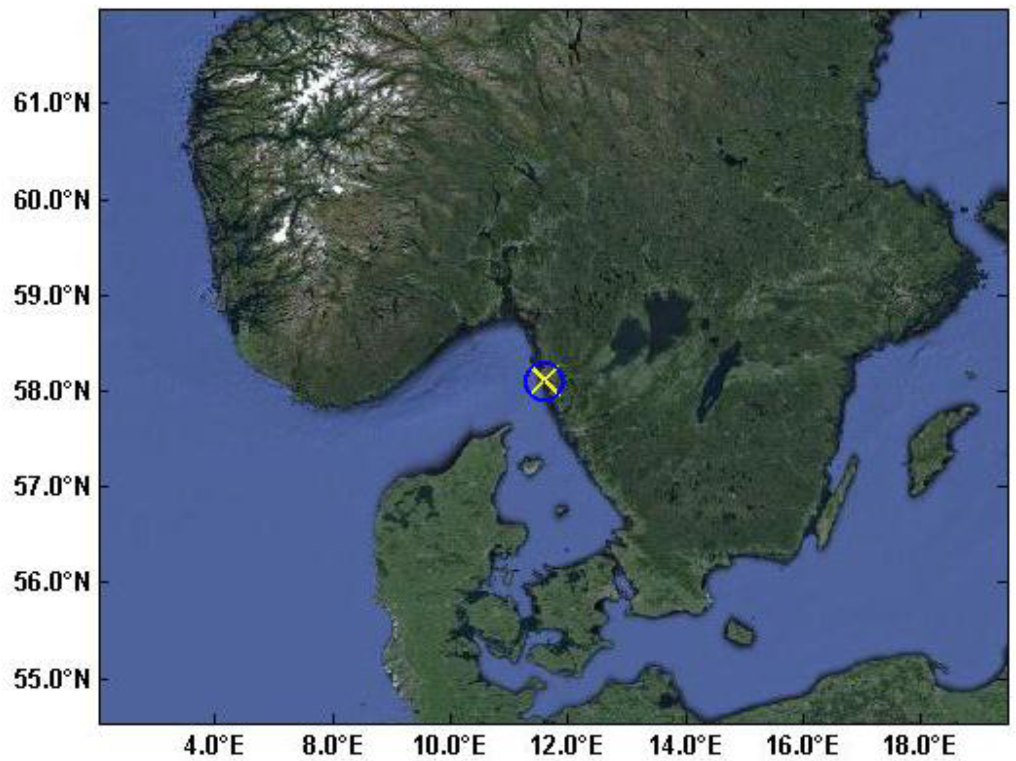
| Site 3 | 57.60°N | 11.63°E | 0.74 m | 3.67 s | 1.83 kW/m | 1 October 1978–10 October 2014 |
| Site 4 | 53.22°N | −9.27°E | 0.73 m | 5.04 s | 1.74 kW/m | 8 May 2008–25 February 2013 |
| Distribution | Site | Parameters | Weights | R-Square | Root Mean Squared Error |
|---|---|---|---|---|---|
| Lognormal-Rayleigh | 1 | −0.619, 0.819 | 0.573 | 0.994 | 0.014 |
| 0.821 | 0.427 | ||||
| 2 | −0.379, 0.657 | 0.761 | 0.975 | 0.042 | |
| 0.996 | 0.239 | ||||
| 3 | −0.938, 0.521 | 0.548 | 0.997 | 0.017 | |
| 0.881 | 0.452 | ||||
| 4 | −0.687, 0.679 | 0.665 | 0.993 | 0.026 | |
| 0.754 | 0.335 | ||||
| Lognormal-Weibull | 1 | −0.598, 1.073 | 0.446 | 0.996 | 0.010 |
| 0.792, 1.661 | 0.554 | ||||
| 2 | −0.374, 1.447 | 0.793 | 0.975 | 0.042 | |
| 0.664, 2.196 | 0.207 | ||||
| 3 | −0.959, 1.205 | 0.512 | 0.997 | 0.017 | |
| 0.504, 1.918 | 0.487 | ||||
| 4 | −0.687, 1.046 | 0.643 | 0.993 | 0.026 | |
| 0.675, 1.903 | 0.357 | ||||
| Rayleigh-Weibull | 1 | 0.425 | 0.318 | 0.997 | 0.010 |
| 1.135, 1.538 | 0.682 | ||||
| 2 | 0.547 | 0.629 | 0.977 | 0.040 | |
| 1.557, 1.907 | 0.371 | ||||
| 3 | 0.332 | 0.506 | 0.963 | 0.064 | |
| 1.213, 1.945 | 0.494 | ||||
| 4 | 0.398 | 0.523 | 0.989 | 0.033 | |
| 1.126, 1.833 | 0.477 |
© 2016 by the authors; licensee MDPI, Basel, Switzerland. This article is an open access article distributed under the terms and conditions of the Creative Commons Attribution (CC-BY) license (http://creativecommons.org/licenses/by/4.0/).
Share and Cite
Li, W.; Isberg, J.; Waters, R.; Engström, J.; Svensson, O.; Leijon, M. Statistical Analysis of Wave Climate Data Using Mixed Distributions and Extreme Wave Prediction. Energies 2016, 9, 396. https://doi.org/10.3390/en9060396
Li W, Isberg J, Waters R, Engström J, Svensson O, Leijon M. Statistical Analysis of Wave Climate Data Using Mixed Distributions and Extreme Wave Prediction. Energies. 2016; 9(6):396. https://doi.org/10.3390/en9060396
Chicago/Turabian StyleLi, Wei, Jan Isberg, Rafael Waters, Jens Engström, Olle Svensson, and Mats Leijon. 2016. "Statistical Analysis of Wave Climate Data Using Mixed Distributions and Extreme Wave Prediction" Energies 9, no. 6: 396. https://doi.org/10.3390/en9060396
APA StyleLi, W., Isberg, J., Waters, R., Engström, J., Svensson, O., & Leijon, M. (2016). Statistical Analysis of Wave Climate Data Using Mixed Distributions and Extreme Wave Prediction. Energies, 9(6), 396. https://doi.org/10.3390/en9060396