1. Introduction
The European Union Renewable Energy Directive 2009/28/EC establishes a policy framework for the production and promotion of energy from renewable sources for the half billion Europeans living in the 28 EU member states. The directive requires that at least 20% of total energy needs in the EU be produced using renewables by 2020, to be achieved in the aggregate by defining various state-specific targets. Such targets are set by taking into account the respective starting points and overall potential for renewables in each member state. The quota of renewable energy in the power mix ranges from 10% in Malta to 49% in Sweden. In Italy the target is set at 17%, starting from a base of 5.7% share of renewable energy in 2005. To meet the EU targets, in 2010 Italy submitted the Italian Renewable Energy Action plan to the European Commission. The plan sets a 2020 target share for renewables across energy sectors as follows: 26.39% in the electricity sector, 17.09% in the heating/cooling sector, and 10.14% in the transport sector. Of relevance to our study is the large potential to increase the share of renewables in heating systems. Nearly 85% of the Italian households still use fossil fuel-based heating systems.
Government authorities are hence concerned about collecting information that can help them design and implement policy instruments that may promote a switch from fossil-based to renewable systems. Given the great diversity of territorial features across the Italian peninsula, geographical factors are likely to determine substantial variation in the propensity to adopt renewables across the population of residential homes. Spatial effects have been found to be significant determinants of households’ heating choices [
1,
2] and can be linked to several factors, such as fuel price differences, heating traditions (e.g., mountain areas usually have strong tradition of firewood-based heating systems), development of the gas grid (usually less developed in rural areas), availability of biomass fuels (stronger in areas located near forests) and different energy needs according to the area (buildings in urbanized areas are generally better insulated as compared to those in rural ones). This study aims to systematically explore such heterogeneity of preferences by means of a geographically explicit choice model estimated from choice experiment data. This study reports the results from a choice experiment investigating household preferences toward different heating systems in Veneto, a region in Northeast Italy with a substantial amount of mountainous territory. The survey data explores preferences for six heating systems: three based on traditional fuels and three based on renewables.
Over the last few years research applications in the field of residential heating based on choice experiments have increased in popularity amongst researchers [
3,
4,
5]. This method enables analysts to investigate preference heterogeneity for different heating systems in terms of energy savings, environmental benefits, comfort considerations, compatibility with daily routines, personal habits and cost. Discrete choice model estimates from the analysis of choice experiments data show how subjects in the sample weight salient aspects in their stated choices. In the presence of a cost for alternatives the data be used to infer the marginal rate of substitutions of attributes with income. This, in our case, is interpreted as the willingness to pay (WTP) for the various heating characteristics described in the experiment. Reference [
3] estimated the WTP for energy-saving measures in residential buildings in Switzerland. In [
6] key parameters (discount rate, intangible costs and degree of heterogeneity) were used to simulate various energy policies. The authors of [
4] focused on microgeneration adoption in the UK and those of [
7] examined the role age plays in terms of behavioral responses towards energy efficiency, in particular whether older individuals are less likely to adopt micro-generation renewable energy technology. References [
1,
8] investigated the choice of energy retrofits in Germany. While [
8] focused on CO
2-saving measures (heating systems and insulation) and WTP for CO
2 savings, Michelsen
et al. [
1] examined driving factors of choice of residential heating systems. In [
5] how different attributes of residential heating systems affect private homeowners’ choice of heating system following renovations was examined.
Whilst several studies have explored group decision making in choice analysis (see [
9] for a reviews of such papers), a common assumption in the stated choice literature is that survey respondents make choices independently of preferences of others. For example, Bartels
et al. [
10,
11] examined the preferences of plumbers and consumers for water heater systems using discrete choice experiments, but treated both samples as if they were independent of each other. Where interdependence between agents has been considered, the assumption has been that the relationship exists between household members (e.g., [
12]), immediate family or close friends. There exists, however, an established literature (e.g., [
13,
14]) accounting for a wider range of spatial interdependencies between individuals, which may induce interdependence of preferences. This induces the phenomenon of socially influenced decision-making: individuals neither act fully independently, nor reach decisions jointly, but they decide based on a mix of social interaction factors, which might be best represented in a succinct manner as geographical determinants.
Over the last ten years or so an increasing body of literature has dealt with the study of spatial effects on welfare changes. Previous studies on this topic mainly focused on addressing the relevance of spatial factors through
post hoc analysis on the WTP estimated from choice models (e.g., [
15,
16,
17,
18]). However, there remains only limited work on the inclusion of spatial variables in the utility structure behind choice (e.g., [
19,
20]). This paper contributes to the filling of this gap: it proposes mixed logit (MXL) specifications to explore how individuals’ sensitivity to key features of heating systems varies in the different geographical areas of the study region. We include not only variables referring to respondents’ geographical location, but also to socio-demographic characteristics of the area in which they live. This allows us to gain further insight on both spatial and social effects on heating systems preferences. To explore the
post hoc validity of our results, we also map the mean values of marginal WTP estimates at the individual level within each area. Detecting if the distribution of benefits is both spatially and socially uneven is useful as it helps policy makers to design geographically targeted programs that are coherent with public preferences.
This is of particular interest in the Veneto region, as both national and local governments have the mandate to design and implement policy measures to foster households’ adoption of energy-efficient and sustainable heating systems, based on renewable resources. These measures can be categorized into economic (e.g., capital grants, tax exemptions, price subsides) and awareness (e.g., education) measures. The latter aim at making households aware of the benefits of energy efficiency, and they attempt to change households’ behavior with respect to fossil fuel consumption. Although financial measures are usually introduced at the national or regional scale, awareness measures can have a local nature (e.g., meeting with citizens, lectures, etc.). Knowing in which areas households are generally less prone to pay a premium to install more sustainable systems would allow policymakers to direct more efficiently their efforts using geographical criteria. This may result in a broader awareness of the importance of the use of renewable resources and in a support over a broader geographical area of government intervention.
The remainder of this paper is organized in four sections:
Section 2 provides an overview of previous studies in the context of spatially explicit discrete choice models.
Section 3 describes the methodology we adopted and motivates the model specification used for the data analysis. In
Section 4 we report and discuss the results. Finally, conclusions are reported in
Section 5.
2. Spatially Explicit Discrete Choice Models: Empirical Applications
There is now compelling evidence that preferences for some environmental goods follow spatial patterns. This may be due to the spatial configuration of such goods and the availability of substitutes [
21] or to residential sorting. People’s preferences for environmental goods can influence where they choose to live, so that measures of preferences tend to be correlated with measures of environmental quality or with distance to environmental amenities [
22]. Recent developments in Geographical Information Systems (GIS) allow researchers to investigate spatial patterns in preferences for environmental goods. Amongst most common approaches is that of investigating spatial distribution of WTP estimates derived from DCE studies. References [
15,
16] used this approach to map WTP estimates for rural landscape features in Ireland. They found evidence of significant global spatial clustering and spatial autocorrelation of the WTP estimates with landscape features that were prevalent in given areas and iconic for local identity being more valued by locals. Reference [
23] investigated spatial heterogeneity in WTP for forest attributes in France. Data on forest distance from respondent’s homes was used in [
24] to capture spatial effects in WTP for enhancement of biodiversity in forests of New Zealand. The authors found evidence of distance-decay effects, that is, respondents living closer to the environmental good being evaluated tend to have a higher WTP for it. The outcomes of targeting agricultural land preservation by using four different strategies for spatial provision of environmental services in Delaware were mapped in [
25]. Reference [
26] used local indicators of spatial association to explore WTP hot spots. Evidence of distance decay on WTP estimates for forest attributes in Poland was found in [
18]. Spatial effects on WTP estimates have been also investigated including spatial variables in discrete choice models. Thus, Hanley
et al. [
27] included a distance parameter in a CV study to estimate distance-decay functions for a reduction in low flow problems on the River Mimram, England, while [
28] included in discrete choice models spatial variables aimed at investigating directional effects on distance decay of WTP values, related to the availability of substitute sites across the region and [
29] included spatial variables as covariates in a discrete choice model to estimate the spatial pattern of the willingness to provide ecosystem services in agricultural landscapes.
Other studies investigated spatial effects including spatial attributes in stated preferences scenarios. The authors of [
30] examined visitors’ preferences for forest management at five adjacent municipal recreation sites in Finland, using a spatially explicit choice experiment. They included site specific levels of attributes to evaluate whether preferences towards management options differed across sites. In [
31] discrete choice experiments were used to examine preferences for the spatial provision of local environmental improvements in the context of regeneration policies. They included the spatial scope of the policy as an attribute, making the trade-off between environmental amenity and its spatial provision explicit. Reference [
32] included the distance from respondents’ home as an attribute to investigate distance decay effects on preferences towards cost management programs in UK. In [
28] WTP was evaluated for improvements in the provision of environmental services of eleven lakes in a lake district in the Netherlands. They included the lakes as different labelled alternatives in choice sets. Finally, spatial effects on preferences for wind power are commonly investigated by including in the choice experiment attributes describing the distance between wind farms and residential areas or shores to account for visual intrusion (see [
33] for a review).
4. The Model
Within the choice experiment approach each respondent’s choice is modelled as a function of the attributes using Random Utility Theory [
47,
48]. According to the theory, for and individual
n facing a set of
J alternatives, denoted by
j = 1, …,
J the utility of choosing the alternative
i is a function of the
K attributes used to describe alternative
j. The utility function has a systematic part
Vni (indirect utility) and a random part
εni, for all unobserved variables, such that:
The systematic part of the utility function of individual
n associated with the selected alternative
i is modeled as a linear function of the vector of the attributes
xi and associated parameters
βn. If the unobserved error term
εni is assumed to be independently identically distributed (i.i.d.) extreme value type I, the probability of individual
n choosing alternative
i out of
J alternatives can be defined by the conditional logit (CL) model:
A property of the CL model is the independence of irrelevant alternatives (IIA), which is most often undesirable as it implies constant share elasticities. The mixed logit (MXL) model [
49,
50] allows for a relaxation of the IIA assumption, whilst continuing to assume the residual error term is i.i.d. extreme value type I distributed. The MXL model allows for unattributable heterogeneous preferences (
i.e., unlike interaction effects, preferences are assumed to be randomly distributed over the population). Different interpretations have been given to the MXL in various empirical work, the two most common interpretations being the random parameter logit (RPL) and error component logit (ECL) models. Whilst mathematical equivalent [
51], the respective behavioural interpretations of the two models are motivated by distinct analytical interests [
52]. More specifically, RPL appeals to the analysis of taste variation, whilst the ECL interpretation is more amenable to the analysis of complex substitution patterns and variance-covariance structure. Behaviourally sound models often mix the RPL and ECL features to achieve flexible specifications that are suitable for the problem at hand. In this spirit we use two separate sources of randomness, one linked to diversity across respondents, the other shared across respondents from the same geographical area.
The utility structure is specified as:
where
and
are vectors of observed variables relating to alternative
i, is a vector of fixed coefficients,
is a vector of random terms with mean
µ and stochastic components that, along with
define the stochastic portion of utility as well as the manner in which utility is correlated across respondents via the unobserved portion of utility.
What makes this model explicit in its geographical variables is that
has a stochastic component
with standard deviation that is in part constant and in part shifted by
, linked to the
hth place of residence via the indicator vector
. The parameter
expands or shrinks the total standard deviation tailoring it to the place of residence indicated by
. In essence:
The aim of the study is to investigate how the variance of the random parameters changes according to different areas of the region. In particular, we focus on the variance shift of key random taste parameters: the coefficient for the cost of heating system and that for the CO2 emission. The first relates to the marginal utility of income, the second to the marginal utility of emission abatement. Importantly for a geographical tailoring of the subsidy policies, geographical differences in the random cost parameter allow us to better investigate how the marginal WTP estimates vary across the region.
Under this basic specification each person has her own parameter , which deviates from the population mean by . The idiosyncratic random term is normally distributed and has standard deviation with mean 0. Variance reducing sites will have , while variance increasing ones .
To define the geographical areas affecting the variance of we used three different criteria to capture both spatial and social effects. We grouped the municipalities of the region according to three criteria: (1) altitude, i.e., being located in low land (plain or valley), hilly or mountainous area; (2) average income in the municipality; (3) population size. Accordingly, we estimated three MXL models. The first criterion produced three different areas, the second and the third ten areas each. Average income was divided in ten classes of €1,000 width, ranging from €15,000 to €25,000. The population size classes are move in steps of 5000 people, with boundary classes being less than 5000 and over 40,000.
Model identification was ensured by keeping as baseline hilly areas for the first criterion, the lowest average income segment (less than €15,000) and the lowest population size (less than 5000 people).
4.1. Expected Results and Rationale
We now turn to our expected results for selected features of the investigation and the rationale behind each expectation. From the altitude-related model we expect individuals living in mountainous areas to be relatively more homogenous in their views on cost of heating system. The motivation would be that populations in these areas are traditionally quite careful with resource use and management because of their harsh living conditions and close-nit societies who often openly disapprove of profligacy. We did not have a clear expectation with respect to residents in hills and plains, although we suspected that there would be a gradient of heterogeneity with the largest being associated with lower altitude. With respect to preference variation of CO2 emissions, we expected that people in the plains be more homogeneous since they are more exposed to air pollution than people in the hills or mountains, especially during the periodical winter fogs that impede speed of transport, often dramatically. Even though fogs are not directly caused by CO2 emissions, smog (smoke + fog) is strongly correlated with CO2.
We now turn our attention to the effect of segregating sites on the basis of average income. For the heterogeneity of cost coefficient, we expect that as income increases the variation of taste intensity for income should also increase as income has been found to be a typical source of heteroscedasticity in economic datasets. The cost coefficient in linear utility specifications is equivalent to the (negative of) marginal utility of income. Relatively poorer residents have little choice in the way they value their last unit of income, while those relatively better off can choose from a wider range of behaviors. A rich person can behave as a miser, but a poor person has no choice. Turning to heterogeneity for the CO2 coefficient we hold much weaker expectations. It can be argued that in richer sites there might be more disposable income and in as much as fewer emissions and a cleaner environment are a luxury good (as the literature on the environmental Kuznets curve suggests) a higher consensus in favor of renewables should be found in richer locations.
The population gradient criterion should suggest that for both coefficients there should be a higher heterogeneity the higher the population, if anything because population size correlates with diversity. Extreme views on utility of income and CO2 emissions ought to be more common in larger size locations. However, it might also be that higher density induces more homogeneity of views against higher levels of pollution. In any case, we do not hold strong expectations along this segregation criterion and which feature will prevail remains an empirical question the outcome of which has weak theoretical basis.
4.2. Ex-Post Validation
The sequence of choices made by each respondent contains additional information that may help improve the accuracy of estimates derived from the latent utility, such as individual specific marginal WTP estimates. These can be used to assess the theoretical validity of the stated choice method by exploring how mWTP estimates correlate with theoretically meaningful independent variables, as suggested in the early literature of validation of hypothetical choice statements [
53,
54]. In practice one can use visual inspection and regression analysis, we opt for both and use geographical mapping and kernels densities. The technical details are as follows. We simulated the population distributions of individual specific estimates of mWTP
n by generating 10,000 pseudo-random draws from the unconditional distribution of the estimated parameters and we calculated individual-specific estimates for each draw as explained in the seminal literature of panel choice models [
50,
55,
56]. The formula employed [
57] is:
where
R is the number of replications (
i.e., draws of
),
is the
rth draw for the CO
2 attribute,
is the observed sequence of choice data by respondent
n,
is likelihood of an individual’s sequence of choices computed at draw
and
is the
rth draw for the investment cost attribute, that is the payment vehicle used to compute the mWTPs.
The individual value estimates are averaged by geographical polygon of each municipality, colour-coded and mapped with ArcGIS to obtain the geographic distribution of the estimates. Kernel density distributions of mWTP from the best performing model are obtained conditional on income levels, altitudes of place of residence and population size of the place of residence.
5. Results
All MXL estimates were obtained by simulated maximum likelihood using the Pythonbiogeme software [
58]. The choice probabilities are simulated in the sample log-likelihood with 1000 pseudo-random draws. We estimated three specifications, one for each criterion by using different
in the standard deviation for the random parameters for cost and CO
2 emissions.
In the first MXL model, which relates to altitude of place of residence of the respondent, denotes the coefficient for mountain areas associated with , while is the analogue for low land. So, the baseline standard deviation is for intermediate altitude areas (hilly). The second (average income) and third (population size) models have 10 ordinal groupings each, so nine are used. In all models error components are assumed to have a standard normal distribution. As the aim of the study is to investigate the heterogeneity of sensitivities for the investment cost and the CO2 emissions, we kept all other coefficients fixed. All models include six alternative specific constants (ASCs) for all heating systems except for LP gas, which is the baseline.
Table 4 shows the estimates for the MNL and the three MXL models. Each of the three MXL models substantially improves the fit to the data. Across the three MXL models, the specification based on population size seems to perform best, according to all criteria. In all the models, the investment and operating cost coefficients are significant and negative, as expected. The other significant determinants of preferences towards heating systems are the emission of CO
2 and required own work. The negative sign for emissions coefficient (FP and CO
2) are as expected, but that for FP is never significant, while the one for CO
2 always is, suggesting a different sensitivity to the type of pollutant caused by heating systems and a preference for technologies that target CO
2 emissions. The coefficient for required own work is also negative, suggesting an expected preference for low maintenance systems.
The alternative specific constants (ASCs) reflect the average system-specific impacts of unobserved factors associated with each system and measured with respect to LPG. These estimates are always statistically significant except for chip wood. The signs of the ASCs for firewood, wood pellet, and methane are positive, thus suggesting that those heating systems are preferred to the LPG fueled ones. Only the ASC for the oil based systems is negative, suggesting that it is the least preferred heating system. The standard deviations of random components are significant in each of the three models, thus suggesting heterogeneity of cost sensitivity in the sample for both investment cost and CO2 emissions. The estimated values for show the sensitivity of the variance of the random coefficients for investment cost and CO2 emissions across the geographical indicators of interest, which we now examine in turn.
In the “altitude” model all estimates for are significant, suggesting that density of coefficient values differs across the three altitude categories. is associated with the variance of investment cost for respondents in mountain areas (−0.019) and is its analogue for the plains (0.025). The alternate sign suggests a monotonic relationship between preference heterogeneity and altitude: the lower the latter the higher the former. In other words, these value estimates are consistent with a lower variance among respondents living in mountainous areas compared to those living in the low land, with those in the hills having an intermediate degree of heterogeneity thus confirming our expectation: preferences for marginal utility of money are more homogeneous in high altitude areas than elsewhere.
The pattern reverses for heterogeneity of taste for emissions, which displays a positive, rather than negative, monotonic relationship with altitude. People living in mountainous areas are more diverse in preference (0.033) compared to those living in the hills and plains. The latter show a higher homogeneity (−0.025) of taste in their view on CO
2 emissions. This differences in spread of taste parameters may be explained by considering that Veneto mountainous areas are less urbanized and populated (and therefore with more diffuse pollution), as compared to the hills and plains. So, extreme views are more prevalent in mountain areas where you might have a wider diversity of perceptions on the emission problem, whereas residents in the plains display higher converge in opinion. This may induce respondents living in the mountains to consider heating systems’ emissions with a broader difference of opinion, thereby requiring a higher policy effort from the viewpoint of education and generally adopt more sustainable heating systems. The seventh to eighth columns of
Table 4 show coefficient estimates for the “average income” model. The lowest segment of income (less than €15,000) was defined as the baseline; eight out of nine investment cost coefficients and five out of nine CO
2 emissions coefficients show significant estimates. All α coefficients associated with investment cost are positive, and their relative values confirm the theoretical expectation of a gradual increase in heterogeneity with respect to marginal utility of money as average income increases. We take this result as a strong endorsement of theoretical validity of this stated preference data.
Finally, turning to the “population size” estimates (columns 10–12), four of the nine investment cost coefficients are significant and these show a monotonic set of relative values with respect to population size. A similar pattern, albeit with inverse correlation, is found for the eight coefficients with good significance for CO2 emissions. The values of heterogeneity coefficients decrease as we move from less to more populated areas, thereby suggesting that in bigger cities people are more heterogeneous in their preferences towards CO2 emissions. As expected, more populated cities are usually more urbanized and therefore more polluted. This may explain why individuals living in those areas are more sensitive to the issue of CO2 emissions, even those produced by heating systems.
5.1. Individual WTP Estimates
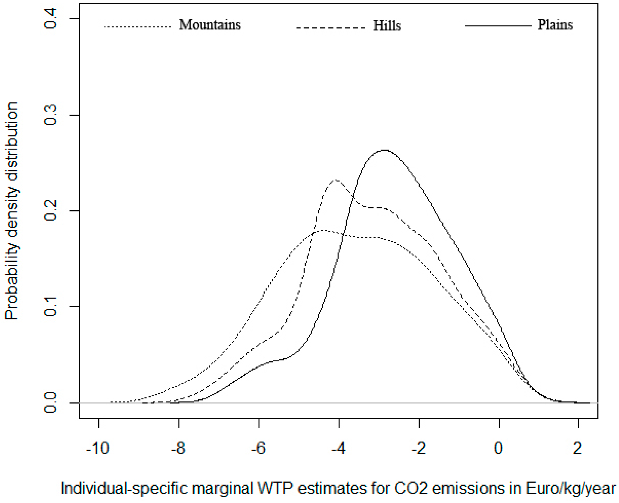
Figure 1,
Figure 2 and
Figure 3 describe the sample distributions of individual-specific mWTP, retrieved from the best MXL specification: the one with heterogeneity by population size. The individual level estimates were computed by using the software tool developed by [
59]. The reported kernel densities uncover differences between the distributions of mWTP values to avoid the emission of 1 kg/year of CO
2 for respondents from the mountains, hills and plains (
Figure 1). Note that because mWTP is computed as a function of both random coefficients, the relatively higher homogeneity of preferences for residents in the mountain for the random cost coefficient is offset by the relatively lower homogeneity of the random coefficient for CO
2 emissions. As such, we cannot expect the distribution of these values to display the pattern of kurtosis previously revealed in the values of estimates for
. By inspecting the figure it is apparent that residents in the plains and the hills have higher frequencies for lower mWTP values for emission reduction, while residents of the mountains have higher frequency in the higher range (in absolute terms) of mWTP values. This suggests that in the mountains there is preference for being able to emit less. Residents of the plains have lower modal values of mWTP with higher frequency around the mode.
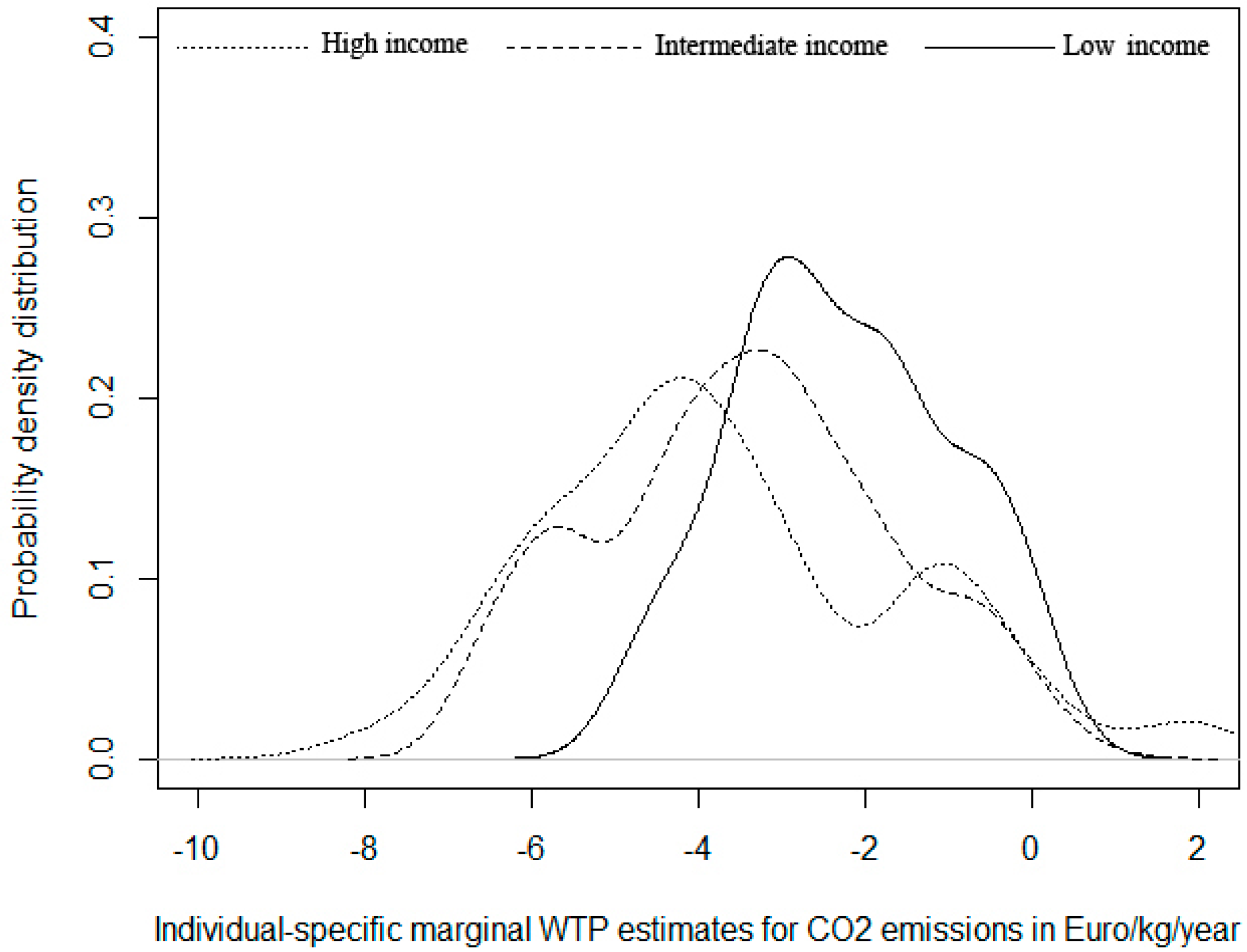
Figure 2 shows the kernel distributions for those respondents characterized by different income levels. We aggregate respondents in three segments: low yearly income (less than €18,000), intermediate income (€18,000–€21,000) and high income (more than €21,000). The distributions show very similar modal values. However, the skewness varies and so does the kurtosis and the presence of local modal values. It is interesting to note that the only income group with higher density of positive values (
i.e., in favor of emission increase) is the one with highest income, which also displays the highest variance and bi-modality. They are the only group with high density for WTP to avoid emission higher than €8. The distribution with stronger positive skewness is that of lowest income, which also displays highest homogeneity of preference (low variance and range) with none being willing to pay more than €6. The intermediate income group displays features in between the other two.
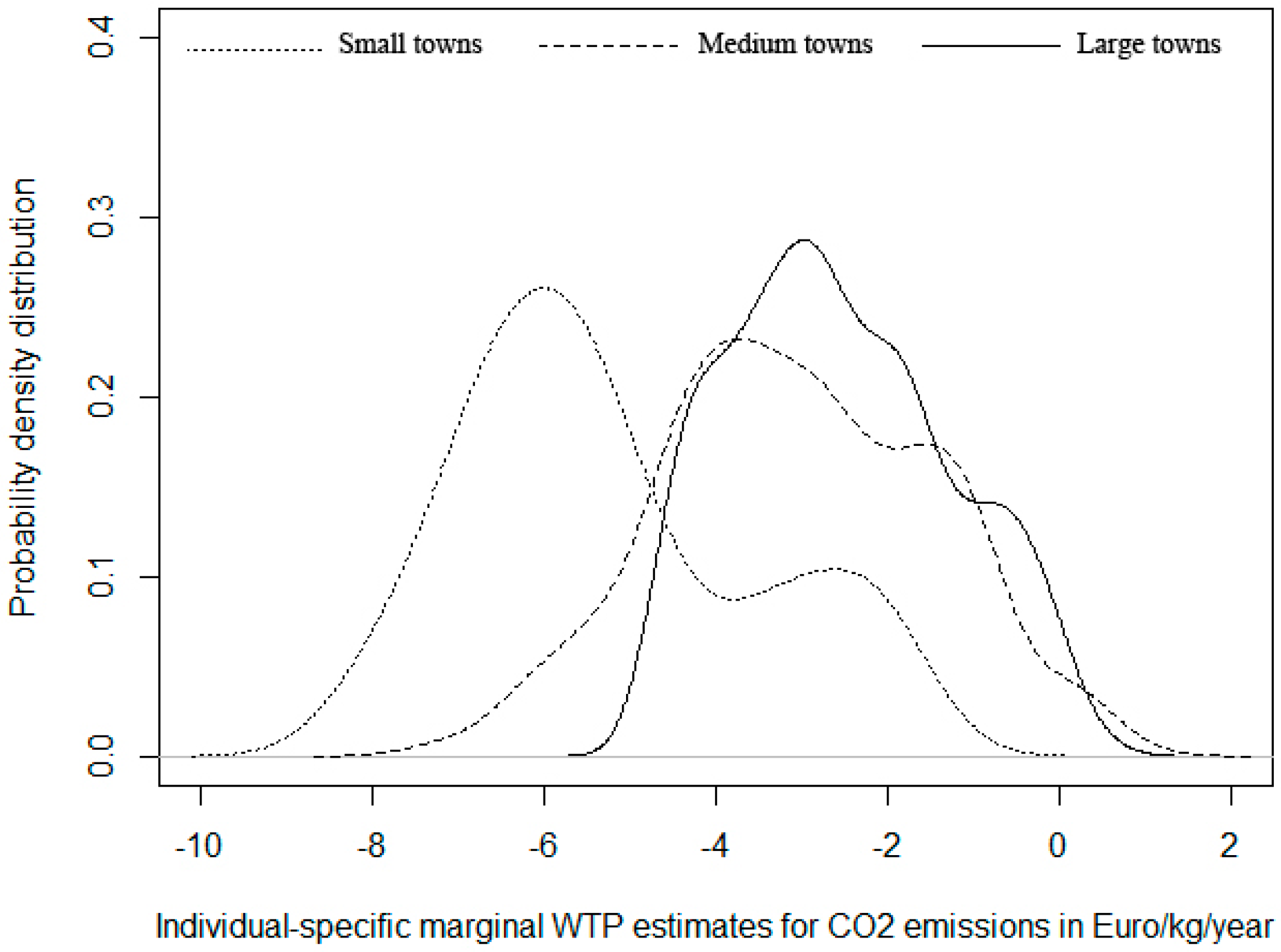
Figure 3 shows the kernel distributions for town residents separated by population size, with towns with small (less than 10,000), intermediate (between 10,000 and 25,000) or large (more than 25,000) populations. Interestingly, this plot shows a higher degree of heterogeneity, as compared to the previous ones. Small town residents have no frequency in positive values, which implies no propensity to increase emissions. They also display largest variation and bimodality, with a modal value strongly shifted to the left of the modes of the other two town size, which overlap. This implies a much higher mWTP for emission reduction. The largest population size towns show highest homogeneity.
5.2. Validation and Calibration of mWTP Estimates
Estimates of individual specific
to avoid CO
2 emissions should be meaningfully related to those variables that are—at least in theory—determining WTP. In order to establish if this is so in our case we report the results of an OLS regression of
on a selected sub-set of socio-economic covariates, which include also indicators for altitude and population size. Instead of average income of the location of residence we prefer to include personal income of the respondent, and because of missing data on this variable, the sample is somewhat smaller (223 fewer respondents) than that used for estimation of the choice models.
Table 5 reports the OLS estimates, whose signs support the validity of the
estimates. Increased education attainment is progressively related to higher values of
, as is personal income and being resident in the plains and in larger towns. Being a male respondent or of different age has no significant effect on
while being from the mountains, everything else being equal, shows a significantly lower
. This seems in contrast with the unconditional distribution displayed in
Figure 1, but the marginal effect of altitude, obtained while controlling for other variables, is obviously different from its unconditional effect.
In order to use estimates obtained by hypothetical statements for policy analysis it is necessary to calibrate them in order to reduce hypothetical bias. WTP estimates from hypothetical statements are typically larger than equivalent estimates obtained from revealed preference data. Several studies have investigated the regularity of such discrepancy and derived calibration factors [
60,
61]. In the context of environmental goods, with which respondents seldom have familiarity, calibration is obviously particularly important. A comprehensive meta-analysis study of environmental nonmarket estimates is that of [
60], in which they find “
a median ratio of hypothetical to actual value of only 1.35, and the distribution has severe positive skewness”. So, in our calibration, the median value serves as the anchoring point which is deflated so that the hypothetical estimate is 1.35 times the calibrated estimate. We then impose a positive skewness on the calibrated values. Hypothetical value estimates falling in percentiles above the median are deflated in increments of 7% every steps of five percentile points, while values below the median are deflated in decrements of 5% for the same percentile steps.
5.3. Geographical Distributions of WTP for CO2 Emissions
In this section we explore the geographical distribution of benefits that would derive if all respondents changed to more sustainable (lower CO
2 emitting) heating systems. The assumption is that respondents move from the current heating system—the data for which were collected in during the interviews—to the nearest system with lower emissions. So, for example, a respondent who reported to be currently using an oil-based system emitting 4575 kg of CO
2/year would move to a more sustainable system within the oil-based group emitting only 3900 kg/year. Someone else that was already at the lowest range of emission within a category (
i.e., methane with 3000 kg/year) would lower emissions by switching to the worse emitter in the more sustainable system in the renewable category (
i.e., a pellet based system emitting 525 kg/year of CO
2). In this manner we can approximate linearly the monetary change by using the individual specific estimates of marginal WTP obtained from the best performing mode, after suitable calibration for reducing hypothetical bias. The computation of the mWTP per kg of CO
2 used the following formula:
where
Is the calibration function (a coefficient consistent with the median value and skewness from [
60]) that adequately deflates the estimate, and
is the marginal reduction in CO
2, conditional on the heating system currently employed by the respondent (in kg of CO
2/year). These were developed by assuming that the length of time respondents signalled to be away from the next adoption decision was an indication of pollution emission levels, with longer times indicating more sustainable current systems (with lower emissions).
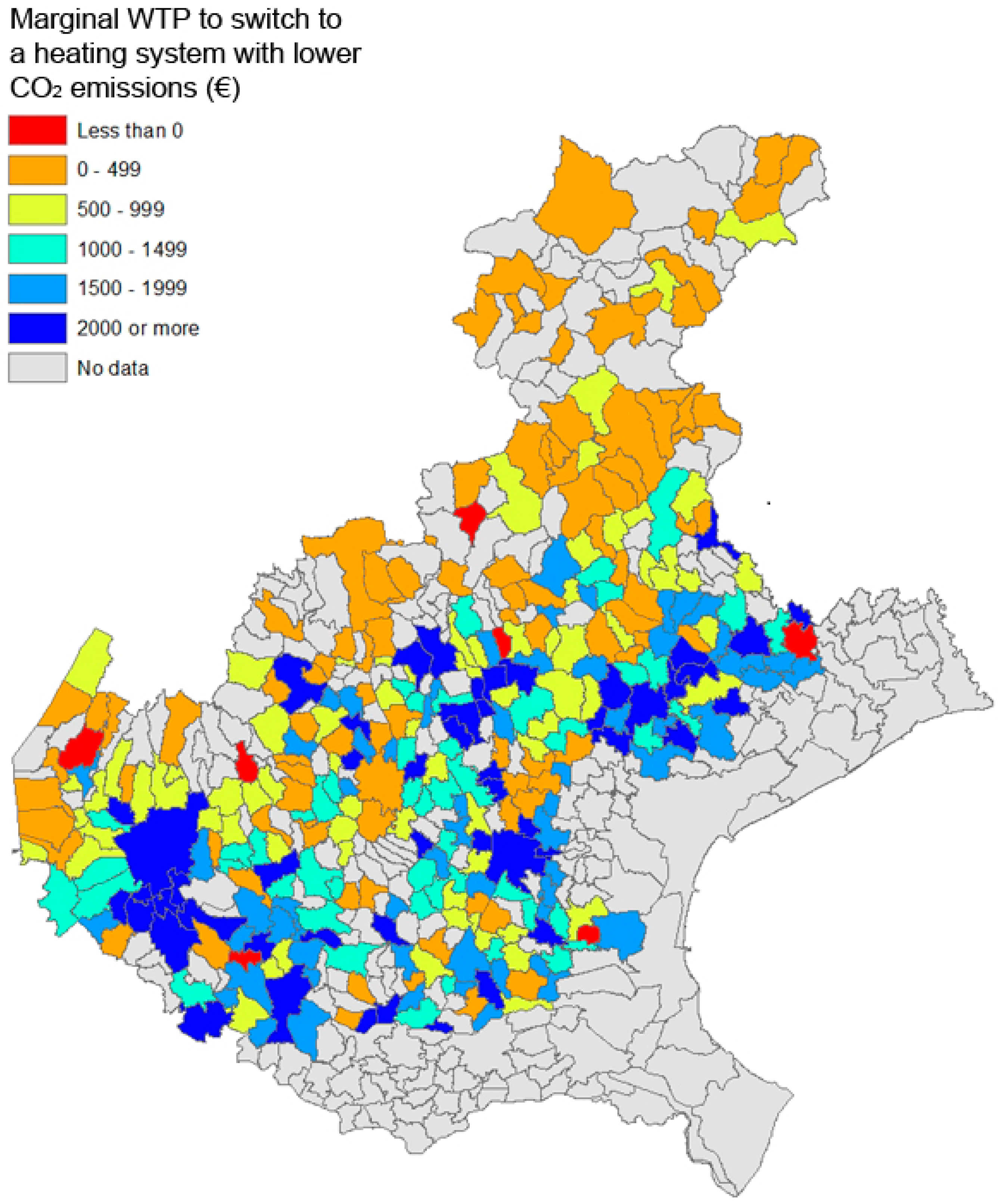
To explore the geographical distribution of the benefits from such hypothetical emission reduction we mapped the values across the territory of the target population (
Figure 4). The map describes the municipality boundaries and the colouring reflects the averaged values from respondents within each boundary. It is apparent that the highest benefits from emission reduction occur in the low land in the south part of the map, and it is especially high in the large municipalities, such as the city of Verona and Padua. The lowest benefits, instead, occur in the mountainous north and along the hilly regions along the foot of the mountains. This might be counter-intuitive if compared with the distributions reported in
Figure 1 and
Figure 2, but it is mostly due to higher deflation values of
that apply to higher
, which are more prevalent at higher altitudes.
6. Conclusions
Emissions from heating systems are large contributors to the level of stock pollutants of the greenhouse gas type. Climate change is responsible for severe damage in high altitude areas, in the form of faster landslides, change in the snowfall patterns and topsoil erosion. However, in the plains air pollution is often more visible for the prevalence of winter fogs and low altitude haze. Respiratory problems are also more common in the lowlands. These factors, along with different patterns of population structure across these areas make geographical factors important in effective policy design. Stated preference methods are increasingly common in exploring nonmarket benefits associated with environmental policies. In this study we collect data on choice of heating systems across the population of Veneto in North-Eastern Italy. This densely populated region covers a wide range of altitudes, from the Alps to the lowlands of the rivers. Such diversity of microclimates induces a differentiated demand in terms of heating systems. As such it lends itself to studying the geographical distribution of policy actions aimed at a more sustainable pattern of adoption of heating systems and its nonmarket benefits.
We developed a choice experiment survey to explicitly address the geographical dimension of taste heterogeneity across residents for the existing heating systems and potential adoptions of more sustainable ones. This required a complex experimental design, which nevertheless provided the identification of the parameters for all attributes and heating systems. In particular, from the methodological viewpoint, we proposed an MXL model specification to account for the role of spatial and socio-demographical factors in respondents’ heterogeneity of preferences towards key features of heating systems. Although our model cannot be considered a proper spatial model, it represents a way to inform discrete choice models with variables related to geographical features. This is important as the existence of spatial effect on welfare changes is well established in literature, but poorly explored in empirical studies. The estimation of spatial discrete choice models has still received little attention in literature, and our paper is an explorative work in such direction.
The hypothesis that justified our work is that spatial variables such altitude, average income and population size of the municipality are sources of heterogeneity of preferences towards key features of heating systems.
Our results show that the variables we consider are in fact a source of variation in the spread of sensitivity to cost and CO2 emissions. In particular, we found that respondents living at higher altitudes display a wider range of preferences than those in the lowlands. We validated our structural model as well as its ex-post values at the individual level by developing theoretical expectation with regards to key variables, such as income and education, which are confirmed by the results. We hence argued that the model and data are theoretically valid.
From a policy viewpoint, our results are of particular interest considering that both local and national governments are providing financial incentives to encourage the installation of energy-efficient and more sustainable heating systems. Being able to account for spatial differences in the perception of the benefits of such measures is useful to design programs that are coherent with public preferences. Furthermore, as some of these measures have a strong local connotation, our results can be useful to help policy maker in addressing their action locally. In particular, our findings suggest that geographical features matter for the adoption of sustainable heating systems and that government intervention should be developed taking this into serious account.


