Abstract
Cogeneration and trigeneration plants are widely recognized as promising technologies for increasing energy efficiency in buildings. However, their overall potential is scarcely exploited, due to the difficulties in achieving economic viability and the risk of investment related to uncertainties in future energy loads and prices. Several stochastic optimization models have been proposed in the literature to account for uncertainties, but these instruments share in a common reliance on user-defined probability functions for each stochastic parameter. Being such functions hard to predict, in this paper an analysis of the influence of erroneous estimation of the uncertain energy loads and prices on the optimal plant design and operation is proposed. With reference to a hotel building, a number of realistic scenarios is developed, exploring all the most frequent errors occurring in the estimation of energy loads and prices. Then, profit-oriented optimizations are performed for the examined scenarios, by means of a deterministic mixed integer linear programming algorithm. From a comparison between the achieved results, it emerges that: (i) the plant profitability is prevalently influenced by the average “spark-spread” (i.e., ratio between electricity and fuel price) and, secondarily, from the shape of the daily price profiles; (ii) the “optimal sizes” of the main components are scarcely influenced by the daily load profiles, while they are more strictly related with the average “power to heat” and “power to cooling” ratios of the building.
1. Introduction
Combined Heat and Power (CHP) is a mature and well established technology for the rational use of energy, with a high penetration in the industrial sector for more than 50 years. At meantime, cogeneration and trigeneration (i.e., Combined Heating, Cooling and Power, CHCP) systems are widely recognized to have a strong penetration potential in the civil sector, and in particular for buildings in the tertiary sector, due to the higher required capacity and the more regular heating/cooling load profiles, compared to residential buildings [1]. However, in most of industrialized countries their penetration in the civil sector still remains well below the recognized potential. This is primarily due to the high capital investment required by CHP and CHCP projects (mainly related with the high cost of the Power Generation Units, PGUs, and the ABSorption chillers, ABSs), which makes it difficult to achieve economic viability [2]. The main difficulties can be identified at two different levels, which are: (i) designing and operating the system; and (ii) dealing with the uncertainties and the associated risks of investment.
As concerns the former of these two problems, it should be observed that plant profitability mainly results from the energy cost savings achieved due to the efficient energy conversion. Thus, it is necessary to ensure that the co/trigeneration plants achieve very high efficiencies, under their real operating conditions. In order to achieve this goal, the energy outputs must be fully exploited, and heat discarded with exhaust gases or, in case of Internal Combustion Engine (ICE) PGUs, via external radiators, should be avoided or limited. Unfortunately, this is not easy and not always cost effective. In fact, most of the small-scale CHP PGUs produce combined heat and power, that are required by the served building and its occupants according to independent and very irregular seasonal and daily load profiles. Therefore, in general, the outputs from the CHP unit do not exactly match the energy demands from the building. Also, as electricity prices vary highly on daily (between peak and off-peak hours) and seasonal bases, the margins for profitable operation of the CHP unit also vary continuously. As concerns plant design (i.e., the selection of the components and their size), further degrees of freedom exist, since it is rarely convenient to size the PGU and the ABS units based on the peak loads, being in any case back-up units like heat-only boilers and vapour compression chillers included in the plant lay-out (for the purpose of providing more flexible operation, redundancy and safety of supply). Then, the problem of optimal design and operation of Building CHP (BCHP) and CHCP systems is a complex task, which has stimulated the efforts of researchers in the last two decades. The proposed approaches may be classified into: (a) simple rule-based design and operation; and (b) optimal/near optimal design and operation. The former class includes a number of instruments developed to provide “reasonable” solutions; such instruments are usually based on interpretative arguments related to the interaction between the plant and the served building. As concerns the components’ sizing problem, approaches based on the duration/cumulative curve of heat demand have been proposed, adopting in particular the Maximum Rectangle Method (MRM) [3] or other hybrid curves accounting for economic aspects [4]. As concerns the plant operation, two main conceptual logics have been analysed, that are usually indicated as Following Electric Load (FEL) and Following Thermal Load (FTL) [5], with evident reference to the “prioritised” output.
However, since the rule-base design/sizing and operation strategies underperform the results achievable by optimization models, most of the contributions published in the last few years have proposed algorithms aimed at optimizing (separately or combinedly) the plant lay-out, the components’ sizes and the operation strategy. Although approaches based on evolutionary algorithms [6] and Artificial Neural Networks [7] have been proposed, the mathematical formulation of the problem is very suitable for resolution by mathematical programming techniques, which have represented the largely most disseminated approach. Depending on the desired level of accuracy in the representation of performance curves of components and the decision to include in the problem binary variables (for instance, to indicate the inclusion/exclusion of a unit from the plant lay-out or the “on”/“off” condition of a unit in a generic time step), Linear Programming (LP) [8], Nonlinear Programming (NLP) and Mixed Integer Linear/Nonlinear Programming (MILP/MINLP) [9,10] solvers have been proposed.
Most of the above research lines are quite mature, but they share in common a limit related with the deterministic approach adopted in the problem formulation. It should be considered that input data to the optimization process are represented by performance and cost figures of components, building energy loads and electricity and fuel prices; also, in the case that any support mechanism is available (aimed at rewarding the CHCP plant for either the achieved energy savings or CO2 emission reductions), the algorithm must include it in the cost/revenue evaluation. Most of the optimization algorithms available in literature deal with all these inputs as if they were exactly known a priori, following a so-called deterministic approach. However, in real world applications these data are not known. In particular, energy load profiles depend upon a number of stochastic variables (climatic conditions, building occupants’ behaviour, etc.) while energy prices are highly fluctuating depending on the complex dynamics of energy markets. The difficulty of predicting these input values is even more evident when we consider that the optimization process usually covers the expected technical life of the plant, which for small-medium scale cogeneration and trigeneration systems is typically assumed between 15 and 20 years. It is absolutely intuitive that the results provided by deterministic tools are significantly error-prone, and that private or public investors cannot fully rely upon them for decision making.
This topic is not new in literature, and in the last decade it has stimulated the efforts of researchers in developing “stochastic optimization techniques” to deal with demand and price uncertainties. Morari [11] provided a comprehensive review of the available techniques to take into account aspects related with flexibility, operability, and control into the design procedures of a chemical plant. In [12] a method is described to improve the robustness of energy systems: this is important since strategic planning is necessary for energy technologies with long life times, due to the uncertainties about future developments that could lead to a major reappraisal of costs and efficiencies.
In [13] the concepts of feasibility and flexibility for a trigeneration system were introduced, as indicators to measure the capability of the plant to ensure feasible operation as parameters vary (variations are intended for steady state operation, not referring to the dynamic changes that are usually accounted for by a different concept, i.e., the dynamic resiliency). The authors pointed out that unit over-sizing, thermal storage and flexible reallocation can be used to improve the feasibility and flexibility of trigeneration systems. In a subsequent paper by the same authors [14], the concepts of feasibility and flexibility were applied to the case of demand uncertainties for a CHCP system including heat storage; however, the study adopted different simplifying assumptions, since the demand uncertainty was modelled imposing possible reductions (ranging between 10% and 44%) in the cooling load to be supplied, and the energy loads were described by assuming only a single shape of the daily profiles. A milestone paper on stochastic optimization of cogeneration system is the contribution by Gamou et al. [15], where a first attempt to characterize the stochastic behaviour of building energy loads was made, based on real data derived by an annual measurement campaign for an office building (with maximum electricity demand of about 1000 kW). The authors concluded that the energy loads can be approximated (on an hourly basis) as a normal distribution, centered on the hourly average demand and with 95% of the area in the range of ±20% of the average demand. Once identified the stochastic behaviour of the energy loads, the authors proposed a hierarchical optimization method, with an upper level where equipment capacities and maximum contract utility are optimized (by nonlinear programming) and a lower level where the optimal energy flow rates and on/off status of equipment are optimized (by mixed integer linear programming routines coupled with sensitivity analysis and enumeration methods). These results are interesting since, in absence of data, in a previous paper [16] the same authors had hypothesised the energy loads to follow a binomial distribution. The results presented by Gamou et al. [15] inspired several other works, related with combined heat, cooling and power planning under uncertainty. In [17] a probability constrained multi-objective optimization model was proposed, in order to support decision making for CHCP systems. In this work the aforementioned results by Gamou et al. [15], i.e., the normal distribution with 95% of area in the range of ±20% of the average demand, were acritically applied to all the energy loads (electricity, cooling and heat). The main contribution of this work consist in the inclusion, in a multi-objective optimization model, of “probability constraints” whose violation is admitted as possible with a pre-fixed probability; of course, the higher the reliability level imposed, the worse is the “optimal solution” achieved by the algorithm at its convergence. Another recent study based on the assumption of normal distribution of the stochastic loads proposes an application in the food industry [18]; in this case, however, referring to a restricted number of “standard days” seems absolutely reasonable, since seasonal load fluctuations were moderate, being most of the energy requests dependent upon the productive process. The optimization was performed for a restricted number of parameters, since some strong assumptions were preliminarily made, like the FEL operation strategy that was continuously imposed throughout the operation year. A different approach was proposed in [19], where once assumed a normal distribution of energy loads (based on a unique daily profile of average loads), discretization of the probability distribution was made using nine representative points, and thus including in the MINLP model a summation of terms related to these nine possible load conditions, each one weighted with its relative probability. The study indicates that the optimal capacity of the plant components is scarcely sensitive to the probability distribution of energy loads, being strongly related only with the average demand. However, transposition of this result to the real world applications does not seem easy nor reliable, due to the several simplifying assumptions made. A similar MINLP optimization routine was proposed by the same authors in [20] for a Building CHCP plant; in this case, however, uncertain programming was addressed by the combined use of Monte-Carlo Method (MCM) and mathematical programming. The Monte-Carlo routine operates as an external “energy demand random generator”, whose results are given as inputs to the optimization algorithm. The examined case study is a hotel located in Shanghai, and normal distribution of energy loads was again assumed. Another very interesting study examined the topic from a more accurate “building energy modelling” perspective [21]. The energy loads of the examined office building (located in Atlanta, GA, USA) were calculated by EnergyPlus; however, in order to account for the stochastic behaviour of energy loads, that are strictly related with the stochastic climatic conditions, the authors renounced to simulate the building adopting the Typical Metereological Year (TMY3), created by analysts of the U.S. Department of energy based on surveys conducted at the National Renewable Energy Laboratory aggregating data for 45 years. Conversely, the authors repeatedly simulated the building using fifteen consecutive years of weather data (out of the 45 used to calculate the TMY3), thus deriving a realistic distribution of energy load, at least for the heat and cooling requests more strictly related with weather conditions (stochastic occupants’ behaviour was not included in the study). However, the analysis conducted in this study is strictly based on the assumption of either a TFL or an EFL operation, which as said above typically underperform the results achievable by a less constrained optimization. Two further studies offer a slightly different perspective to the problem of optimization of CHP and CHCP systems under uncertainty. In [22] the optimization was performed assuming a wide set of uncertain parameters, including energy prices; the study, however, is not strictly focused on a single co/trigeneration system, but rather investigates a more general combination of distributed energy systems, also including photovoltaics and solar heat collectors. In [23] a stochastic optimization was performed for a combined heat and power system, by adopting a Multi-Objective Particle Swarm Optimization (MOPSO); the study, however, differs significantly from those presented above, since a “dispatch” problem is addressed, that means, identifying the optimal mix of contribution of different power-only, cogeneration and heat-only units, with pre-fixed capacities, for a specific load condition. In [24] the authors performed a sensitivity analysis and studied the resilience of trigeneration systems, by imposing energy demands variation within the range (−20%, +20%), amortization factor’s variation between 0.10 and 0.30 year−1 and natural gas price fluctuations between 0.015 and 0.035 €/kWh.
Finally, a reference to a very peculiar and interesting study [25] must be given, since it addresses the topic in a very systematic way. This work investigates the characteristics of energy loads and price uncertainties, classifying them on multiple time frames, depending on the magnitude of the uncertainty and the possibility to predict, more or less reliably, the stochastic variables. Long-term time frames, which cover the total life of the plant, were dealt with by assuming alternative scenarios [26]; medium-term time frames adopt partitions of time steps based on seasonality and “day type” (working and non-working days) features, allowing to adopt deterministic approaches for some inputs, like natural gas price, which do not experience rapid fluctuations; short-term time frames accounts for the parameters highly fluctuating in the short term, like electricity price with volatile behaviour.
This extensive literature review on the stochastic optimization of small-medium scale CHP and CHCP system suggests that, besides some very interesting approaches, most of the available contributions reveal:
- -
- A scarce to moderate characterization of the intrinsic features of the stochastic parameters. The probabilistic distribution of energy loads is rarely examined in detail and, in general, trends are studied for a single or very few (up to three, one per climatic season) standard days. This approach has been proven error-prone, since a sufficient number of “standard days” must be selected to achieve optimization results consistent with those that would be obtained adopting a whole set of hourly data for a year [27,28].
- -
- A major focus posed on the mathematical problem, rather than on the actual energetic behaviour of the building and the plant to be installed. This is also proven by the dozens of articles (not discussed in the above literature overview for the sake of brevity) with similar titles but published by “operational research” experts.
Hence, when performing a deterministic optimization for a co/trigeneration system to supply a generic building, an engineer with a good knowledge of the cited literature should know well that the achieved results are not fully reliable (uncertainties having been neglected), but completely ignores the relevance of the eventual errors and the factors that mostly influence it. Even when a conservative approach is pursued by performing ex-post sensitivity analyses, it is not easy for the analyst to identify: (i) the parameters to be varied; (ii) the entity or the “morphology” of the variations to be imposed.
In order to provide a clearer view on such aspects, in this paper the topic of building CHP and CHCP optimization under energy loads and price uncertainties is addressed from a completely different perspective. Indeed, the focus will be given to the most common errors that may occur when developing energy load and price profiles to be used as inputs for the CHCP optimization tool. Complete sets of energy load and price profiles, for 8760 h/year, will be developed for a number of scenarios, resulting from a keen analysis oriented to distinguish between errors related to:
- the shape of the daily energy load profiles;
- the relative weights between heating/electric and cooling/electric loads, respectively in winter and in summer;
- the shape of the daily electricity price profiles;
- the relative price of electricity and fuel.
While the 4th of the above errors has been someway investigated in literature and represents a typical aspect to be addressed by conventional sensitivity analysis, to our knowledge the former three types of errors have been never examined in the literature. The influence of these errors (either considered separately or in combination) on the economic, energetic and environmental results will be studied with the aid of a deterministic optimization tool.
The paper is structured as follows: in Section 2 the deterministic optimization tool will be briefly presented. In Section 3 the case study, the “base case” scenario and all the modified scenarios as concerns energy loads and prices will be clearly analysed. In Section 4 the results of the optimization obtained in the different scenarios will be critically compared by adopting several possible representations at annual and daily basis. Some conclusions will be finally drawn.
2. Fundamental Features of the Deterministic CHCP Optimization Tool
In order to perform the analyses for different scenarios as concerns the uncertain inputs in terms of energy loads and prices, a reliable instrument is adopted, which performs profit oriented optimizations at synthesis, design and operation level. The tool has been presented in details in [29]; then, examining in detail all of its features and the procedure followed to derive the embedded cost and performance figures for plant components is out of the scope of the present section. Conversely, only some fundamental aspects will be here briefly outlined, so as to allow for a more intuitive interpretation of the results presented in the next sections. The reader is invited to read the referenced paper for any further detail on the model. The tool consists of two distinct routines:
- Single-Building Optimization (SBO) routine, which optimizes the synthesis, design and operation of a CHCP plant (equipped with thermal energy storage) serving a specific building;
- Multi-Buildings Optimization (MBO) routine, which optimizes the synthesis, design and operation of an integrated trigeneration plant that includes a number of CHP units serving a cluster of buildings via an electric μgrid and a warm water distribution network.
Both routines are based on Mixed Integer Linear Programming (MILP); obviously, only the SBO routine will be used in this paper, since the analysis proposed in the next sections is performed for a single building. The problems of synthesis (i.e., selection of the components to be included), design (selection of the optimal size/capacity for each component) and operation (selection of the on/off state and load level, for each component and at each time step) are solved at a unique level, since any hierarchic order between routines solving separately each optimization level would have slightly underperformed the solutions achieved by a single-level routine. Also, a main reason for the assumption of a single routine lies in the low computational effort caused by the linear formulation of the problem. The tool requires, as input data, the building requests for heat, cooling and power and the energy prices (sell and purchase prices, separately, if bidirectional grid connection is assumed) on an hourly basis and for a whole year.
2.1. Variables and Objective Function
The SBO routine adopts three redundant superstructures of CHCP plants, which include natural gas or diesel ICEs and gas turbines as possible prime movers, and single or double effect absorption chillers, together with all the main possible auxiliary components. Hence, the optimized variables are as follows:
- −
- At synthesis level, a number of binary [0, 1] variables, indicated as δcomp, whose values “1” and “0” indicate the options to include or not the related component in the optimal plant lay-out;
- −
- At design level, the electric rated capacity of the CHP unit ( in kWe), the cooling capacity of absorption chiller ( in kWc) and the volume of the heat storage tank (VTES in m3) to be installed;
- −
- At operation level, the rated output (i.e., the load level) of each component at any time step (1 h) is optimized. For the heat storage tank, a hourly average charging/discharging rate is assumed as “operation variable”.
The optimal value of the aforementioned variables is obtained by a MILP algorithm, solved by efficient LINDO API 8.0 routines [30]; although a linear formulation of the problem could seemingly affect the reliability of results, it has been proven to achieve efficient solutions and with a moderate consumption of computational resources [29]. The optimization routine assumes as objective function the Net Present Cost (NPC) or, equivalently, the Net Present Value (NPV) of the investment (which is the negative of the Net Present Cost). Then, the objective function includes:
- ○
- The total investment cost, Itot: appropriate linear cost functions are included in a library, developed on the basis of large databases of CHCP components created within previous research activities [31]), so as to express Itot as a function of components’ capacities (i.e., decision variables at design level);
- ○
- The total cost of the fuel consumed over the plant life cycle (assumed to be 15 years), FUELtot, calculated by using annual fuel expenses and summating their values at the “present time” by adopting an appropriate Present Worth Factor (PWF). Of course, FUELtot includes the cost for the fuel consumed by both the CHP unit and the auxiliary boiler(s);
- ○
- The total cost/revenue for the bi-directional power exchange with the grid, Ce.exch, again cumulated and actualized by using the appropriate. No revenues from heat/cooling production are explicitly taken into account, because the CHCP system is assumed not to be connected to any external district heating/cooling network and it cannot consequently sell thermal or cooling energy to external users. However, the “cogenerated” heat and cooling energy obviously contributes to increase the NPV since (i) the recovered heat induces an avoided cost in terms of fuel to the heat-only boiler; and (ii) the cooling production by the absorption chiller induces an avoided electricity consumption in the auxiliary vapor compression chiller;
- ○
- The total maintenance cost, accounted for by assuming an average 0.015 € cost per kWh electricity produced; this value is a reasonable figure for natural gas engines [32].
The profit-oriented optimization routine minimizes the NPC of the plant (or, equivalently, maximizes the NPV).
2.2. Physical Constraints
The feasible space of variables is bounded by a number of physical constraints, which may be grouped as follows:
- −
- Coverage of energy loads: the sum of energy outputs from the different components must be always sufficient to ensure full coverage of energy requests from the building. For instance, the coverage of direct/indirect heat requests is imposed by:where i indicates the time step, H is the thermal output from the prime mover (in kW) in the time step, C is the cooling output by the absorption chiller (that divided by COP gives the heat rate needed to feed this component, thus representing an additional heat load), represents the charging/discharging rate (respectively when negative/positive) during the ith and Dh indicates the heat load. The constraint is imposed as an inequality, in order to allow the algorithm to explore possible solutions where the CHP unit is not strictly operated according to a FTL strategy, and hence some surplus heat can be discarded to the radiator or by exhausting the hot gases. Similar equations are imposed for the coverage of cooling loads (in equality terms, since production of surplus cooling energy is in no case profitable) and for the electrical balance with the grid;
- −
- Production limits: at each time-step, this trivial constraint imposes the production rate of each component not to exceed its rated capacity. For instance, as concerns the CHP unit, we have:where PHRCHP represents the Power to Heat Ratio of the CHP unit. Again, similar equations are imposed for the absorption chiller and the heat storage;
- −
- Heat storage balance: it imposes a relation between the sensible energy stored (STOR) at the beginning of a generic time step “i” and the amount stored at the successive time step “i + 1”:In Equation (3) ∆H% represents an hourly heat loss rate (which depends on the thermal insulation of the tank).
- −
- Congruence between operation and synthesis variables: since each component can be either included or not in the lay-out (depending on the optimal value assumed by the binary 0–1 synthesis variable δcomp), for the CHP unit the following constraint is imposed:This constraint forces the production rate of the CHP unit to zero (for the examined ith time-step) whenever the component is not included in the lay-out (i.e., δcog = 0), while it is not a binding constraint when the CHP unit is included (i.e., δcog = 1), provided that the constant κ is assigned with a conveniently high value (in the order of 105 when Hcog is expressed in kW). Similar constraints are imposed for the absorption chiller and the heat storage tank;
- −
- A number of additional constraints are imposed and not presented here in details for the sake of brevity. Just to provide some brief notes, a first additional condition is related with the technically feasible dynamic operation of the CHP unit: two distinct maximum feasible hourly load variations are imposed, for the ramp-up and ramp-down periods. Such a constraint is imposed to avoid convergence toward solutions that require frequent start-ups and switch-offs of the unit. A second additional (and optional) condition is related with the fulfilment of the eligibility conditions to have the optimized CHCP configuration assessed as “high efficiency cogeneration”, according to the current legislative framework in Europe [33].
The brief analysis of the optimization tool provided in this section is not intended to represent an exhaustive description; the reader is invited to refer to the cited papers [28,29] for further details on the algorithm. For the scopes of the present paper, one of its main features must be underlined: the tool requires 8760 values, on hourly basis and for a whole “standard year”, for each energy load (heat, cooling and electricity) and for the electricity buy and sell prices. These values are dealt with as “deterministic”, and they should be consequently conceived as “average expected values over the technical life of the plant”.
3. The Case Study: Base Case and Alternative Scenarios for the Uncertain Data
In this section the examined case study is introduced, that is represented by a 646 rooms, 1174 beds hotel situated in Rome (latitude 41°56′ N, longitude 12°27′ E). For the examined building, an energy audit had been conducted during a research project [34], following a very simplified but common approach:
- -
- All the historical data related with energy consumption had been collected. They essentially consisted of electricity and natural gas consumption derived from the bills; as concerns electricity, also disaggregated consumption data per tariff band (peak, medium-load and off-peak hours) were available;
- -
- Based on interviews with the hotel management and with the technicians and on comparisons with trends available in literature, typical daily profiles for working and non-working days were developed. These profiles were used to spread the historical consumption data and thus obtain the required 8760-values arrays needed as inputs for the optimization tool.
While at a first glance such an approach could appear quite rough, it must be observed that:
- -
- In large buildings where complex activities take place, any attempt to use more sophisticate approaches (for instance, dynamic simulators of the buildings’ energy performance) would not necessarily provide more reliable load profiles, due to the enormous amounts of hardly predictable data to be collected;
- -
- It is very common, in the energy auditing phase, to base part of the assumptions on the direct contribution provided by the personnel involved in plant operation.
The results achieved by the aforementioned method will be indicated, below in this section, as “base case” energy loads. As concerns the “base case” in terms of electricity prices, they will be assumed as the local electricity prices at 2005 (i.e., the set of data that had been collected, on hourly basis, when the research activities on the CHCP viability in the examined building were started). The reason for assuming, as a reference date, a condition occurred several years ago will be cleared in the Section 2.2; at the moment it is sufficient to clarify the perspective assumed below in the paper.
The analysis will attempt to identify the possible errors occurring in a CHCP feasibility study that could have been developed, in 2005, by an energy analyst who:
- -
- Completely relied upon the energy load input data that were indicated as “base case”, by the interviews-based energy audit;
- -
- Adopted the current (i.e., at the moment when the feasibility study is assumed to be conducted, year 2005) electricity prices and natural gas price.
It is evident that the study proposed in this paper is particularly suited to existing buildings, where such “base case” energy loads can be easily derived. In the next subsections, different deviations between the “base case” and possible alternative scenarios will be defined, in details. All the scenarios will be adopted to conduct CHCP feasibility study in the successive sections.
3.1. Alternative Scenarios Descending from an Erroneous Load Estimation
In this subsection the hypothesis that the “base case” load profiles obtained by the interviews-based procedure described above differ from the actual load profiles is made. In order to make the study more systematic, two specific types of errors will be examined separately:
- −
- “daily profiles’ shape errors”, consisting in an erroneous assumption of the shape of the daily energy load profiles;
- −
- “heating/electricity and cooling/electricity load ratios estimation errors”, consisting in an erroneous estimation of the fraction of electricity consumption that has been used to supply HVAC systems for space heating and cooling.
3.1.1. Daily Energy Load Profiles’ Shape Errors
In this subsection it is assumed that the interviewed plant owner or technician had an erroneous perception about the shape of the daily load profiles, and that consequently the “base case” energy loads is to be considered:
- -
- Correct in terms of total daily loads. This assumption is reasonable, since the simple procedure of dividing the monthly consumption of natural gas or electricity by the number of days of the month (eventually introducing some minor corrections to distinguish between working and non-working days) has not relevant margins of errors;
- -
- Erroneous in terms of hourly loads.
In order to make the analysis more accurate, each energy request will be examined separately.
Then, below in this subsection distinct “shape errors” in the daily load profile will be adopted for the “heat”, “cooling” and “electric” load profiles; also, for the heat loads, two distinct modified trends will be examined for the space heating and the Domestic Hot Water (DHW) requests.
The proposed trends are separately shown in Figure 1a–d (in normalized terms, i.e., by expressing the hourly fractions of the total daily load). It may be observed that the daily profiles indicated as “base case” and suggested by the plant owner/manager are quite flat and regular; consequently, some reasonable changes are imposed to derive four modified daily load profiles, as detailed below:
- As concerns the space heating load (limited to the winter period), it is assumed that a peak request occurs in the early morning hours (6.00–7.00 a.m., see Figure 1a). This is quite typical for the space heating of large rooms or open spaces (like the Conference rooms or the hall of hotels) or, for smaller rooms, when the plant have been switched off during night-time;
- As concerns the DHW requests, an even higher peak can be expected in the early morning, due to the reasonably high simultaneity factor in the sanitary uses of hot water. Let us observe the adopted modified profile significantly differs from the “base case”, which appears quite unrealistic;
- The “base case” daily cooling load profile, which also was very “flat”, was modified to follow a more common trend for civil applications, with significant increases in the cooling requests after 12.00 a.m. and peak loads occurring in the early afternoon;
- As concerns the electric loads, that should be here intended as electricity uses for equipment and appliances (i.e., excluding any electric consumption for Heating, Ventilation and Air Conditioning units, HVACs), just minor changes are imposed, based on shifting part of the night-time consumption to the day-time hours. This assumption reflects a possible realistic condition, in case the plant owner/manager had overestimated the energy requests for internal and external lighting during night-time.
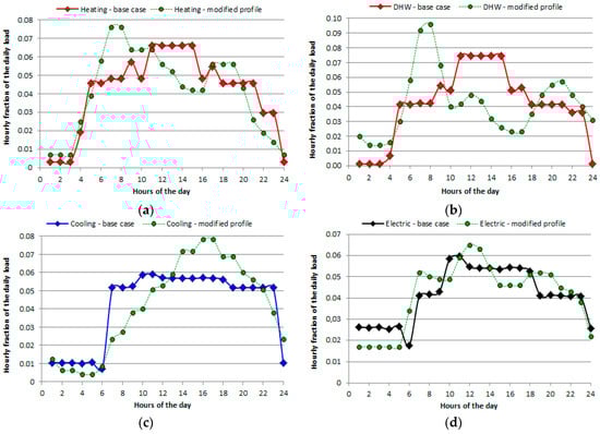
Figure 1.
“Base case” and modified daily load profiles, for the different energy requests: (a) Space heating; (b) Domestic hot water; (c) Space cooling; (d) Electricity for direct use (electric equipment and appliances).
It should be cleared that, in absence of sufficient details on the features of the building envelope and on the daily trends of the number of guests in the hotel, there are no elements available to suppose that the “modified” load profiles are more correct than the “base case” ones. In fact, this section was not aimed at developing more precise or correct load profiles, but just to formulate a realistic hypothesis as concerns possible “shape errors” that could occur in the energy load estimation phase.
3.1.2. Heating/Electricity and Cooling/Electricity Load Ratios Estimation
In this subsection a different type of error, quite common in the energy-auditing phase, is considered. In order to clarify the followed approach, some premise is needed. In existing buildings served by a centralized HVAC system (with a reversible heat pump coupled to a hydronic circuit), it is very common not to have a dedicated electricity meter for the heat pump or chiller. In such cases, there is an intrinsic difficulty in dividing the overall electric consumption into the fractions consumed for “pure electrical uses” (lighting, appliances, etc.) and for “indirect uses”, i.e., to supply the chiller or the reversible heat pump for space cooling and/or heating purposes. When attempting to calculate space heating and cooling loads, the following trivial approach is usually followed:
- -
- a base electric load is estimated as average monthly electric consumption in the “intermediate season” (i.e., in the period where neither space heating nor cooling is requested);
- -
- in the summer and winter periods, such a base electric load is subtracted from the actual electricity consumption derived from the supplier’s bills. This procedure, that implicitly relies upon the quasi-constancy of monthly electricity consumption for lighting and appliances throughout the year, allows to get a rough estimation of the additional electric consumption by the heat pump or the chiller;
- -
- The electric consumption for “indirect uses” is finally used to calculate the space heating and cooling loads, by assuming an appropriate Seasonal Coefficient of Performance (SCOP) or Energy Efficiency Ratio (SEER).
This approach was followed when developing the “base case” load profiles for the examined hotel building. The above procedure, which has some merits related with its simplicity and the consistence of some hypotheses it is based on, evidently implies some margins of error. In this section the following modified scenarios are considered:
- Decreased fraction of electricity consumption for space heating: this modified scenario is based on the assumption that, when deriving the space heating loads following the aforementioned approach, these loads are overestimated by 30%. The resulting modified load profile is shown in Figure 2a, where the load profiles referring to the “base case” are also shown to allow for an easier comparison. In particular, in the figure the curve enveloping the daily peaks of total heat (space heating and DHW) and electric loads are presented. We may observe that the base case and the modified scenario only differ in the winter period (i.e., when space heating is required), and that the modified heat load profile achieves much lower annual peaks (approximately 2200 kW, instead of 3150 kW that is the peak in the base case). A slightly higher electric load consequently results in the winter period, due to the modified shares of actual electrical consumption (derived by bills) between “direct” and “indirect” electrical uses.
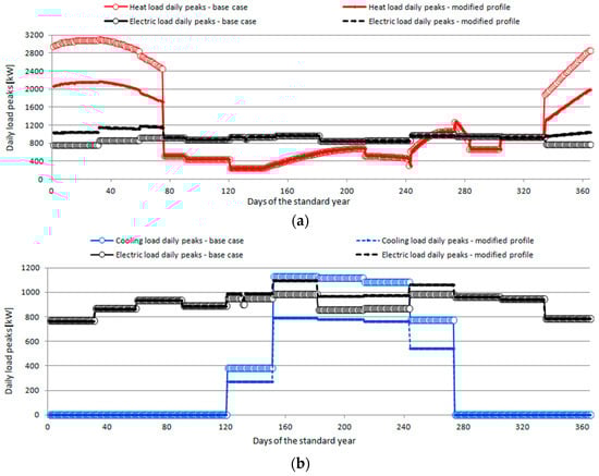 Figure 2. Curves enveloping energy load daily peaks for the “base case” and the modified scenarios: (a) Lower fraction of electricity consumption for space heating; (b) Lower fraction of electricity consumption for space cooling.
 - Decreased fraction of electricity consumption for space cooling: similarly to the previous case, this modified scenario assumes that, when attempting to derive the space cooling loads following the approximate approach, also these loads are overestimated by 30%. The profiles obtained for the lines enveloping the daily load peaks, in this modified scenario and in the base case, can be compared in Figure 2b.
The scope for introducing these scenarios is evident: while such estimation errors are quite common in the energy audit of existing buildings, at meantime they can be expected to influence significantly the results achievable in terms of optimized CHCP configuration and operation. In fact, both of the above scenarios induce significant changes in the buildings “power to heat” or “power to cooling” load ratio; then, the modifications introduced can significantly vary the energy exchange balance with the grid (passing, from instance, from a prevalence of “energy sell” to a prevalence of “energy buy” hours).
3.2. Alternative Scenarios Descending from an Erroneous Price Estimation
As said at the beginning of Section 2, the “base case” electricity prices were assumed as the local prices at 2005. According to the electricity market rules in Italy (which are at some extent harmonized with those in force in most of the member states at European Union level), the energy prices vary, on hourly basis, as a result of variations in the clearing price of electricity market. In particular:
- -
- The energy selling price for a small-medium scale CHP unit may be assumed coincident with the clearing price occurring in the “electrical zone” where the unit is installed (the territory in Italy is divided into six “electrical zones”);
- -
- The energy purchase price is calculated as weighted average of the clearing prices occurring, in the examined hour, in the different electrical zones. However, in order to properly reflect the total cost of the purchased electricity, the additional cost paid for each kWh for the coverage of energy transmission and distribution, the support mechanisms for renewable energy sources and also the Value Added Tax (VAT) should be included.
In order to develop the two “base case” 8760-values arrays (one for the energy sell and one for the energy buy price) needed, as input, from the optimization tool, data at 2005 were derived from the historical reports of the public society that organizes the energy market [35].
In this section the possible error made by an energy analyst that, in absence of further information or reliable forecasts, assumed to design (in 2005) a CHCP plant based on the current prices (i.e., the cited “base case”) is investigated. It is now clear why the present study assumes such a remote (in the past) reference condition and hypothetical date when the plant optimization is assumed to have been performed. In fact, today more than a decade has passed from the reference date, and the energy prices have significantly changed along the years, allowing us to develop a realistic scenario as concerns the error that would have been made. Then, it could be supposed to use, as a “modified energy prices” scenario, the most recent one (complete sets of data already available for 2015). However, the present analysis is not aimed at comparing the results in two particular scenarios, since the conclusions achieved could be of limited interest and difficult to extend to other possible contexts; rather, the available historical price data are used to develop more easy-to-interpret scenarios, each one differing from the “base case” for a specific feature. An accurate analysis of the energy prices observed in the last ten years (period 2005–2015) and the acquired experience on the factors most influencing the viability of CHCP plants suggest us to distinguish between two “types” of errors that may be committed:
- −
- “daily electricity price profiles’ shape errors”, consisting in an erroneous assumption of the shape of the daily electricity price profile, at a same average electricity price;
- −
- variation in the average electricity price or, better, in the ratio between the average electricity price and the fuel price.
3.2.1. Daily Electricity Price Profiles’ Shape Errors
Along the life time span of a CHCP plant, usually assumed in the range between 15 and 20 years, the shape of the daily electricity profile may vary due to a number of external factors. As an example, again referring to the Italian case (but the analysis has an absolutely general value and would remain valid in case that different changes occurred), in the decade between 2005 and 2015 there has been a dramatic change in the morphology of the power production system. Due to the strict relation between the mix of technologies contributing to power generation and the energy prices, this has resulted in deep modifications of the price profiles, especially on a daily basis. In particular:
- -
- In 2005 the national power production system essentially relied upon new generation combined cycle power plants, with obsolete steam plants often operated as “hot reserve” and inefficient gas turbines operating, for a limited time, only to supply peak loads. The penetration of renewable was moderately low, with a large prevalence of “predictable production” units like hydropower plants. This mix of technologies of course resulted in high daily fluctuations of electricity prices between peak and off-peak hours;
- -
- In 2015 the national power production system has observed a dramatic increase in the installed capacity of renewable technologies, which is now higher than 50 GW (accounting for more than 42% of the total installed capacity) and being almost comparable with the annual national peak load, which is approximately 52.5 GW. The new installed renewable capacity has a large prevalence of PhotoVoltaics (PV), more than 19 GW, whose production is obviously limited to peak hours and significantly increases in the summer period. As a consequence, during “peak hours” (i.e., during daytime hours when the national electric demand is highest), large amounts of “green” electricity are available, which have been produced with null or very low operating costs. The effect is intuitive: the daily price profiles have been significantly “smoothed”, with an evident reduction of the ratio between the price observed during peak hours (day-time) and off-peak ones (night-time).
This aspect is very relevant for the feasibility of CHCP plants. In fact, small-medium scale trigeneration systems for buildings application have usually benefitted of the “synchronism” between energy load and price profiles. In other words, as the building and its occupants usually increase their energy request during day-time hours, thus invoking for the CHCP unit to supply more heat/cooling/power, this usually occurred with a good time overlap with the hours where the energy price is higher. When such a correspondence is no longer observed, the feasibility of CHCP plants may be negatively affected. In order to isolate the aspects related with the change in the shape of energy price profiles, the following elaboration was made:
- The average shape of the daily energy prices profiles was calculated in normalized terms, i.e., dividing the hourly prices by a cumulated daily total price, so as to have a series of 24 values (one for each hour) that summed up 1.00. The shape was calculated distinctly for the winter and the summer season, and for both the “base case” (year 2005) and the modified scenario (year 2015). The results obtained are shown in Figure 3. It may be observed that in 2005 the ratio between peak and off-peak prices assumed values in the order of 3.5, while in 2015 it is approximately equal to 1.7, thus confirming the aforementioned smoothing effect induced by the high penetration of photovoltaics;
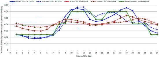 Figure 3. Normalized daily price profiles as concerns energy sell (the presented values refer to 2005 and 2015 and to the winter and summer season) and energy purchase.
 - The normalized profiles derived for 2015 were adopted to develop a new array (with 8760 hourly energy price), but maintaining the same average seasonal electricity prices observed at 2005. In this way, the base case and the newly obtained “modified price profile” only differ for the shape of the daily profile, and not for the average price.
For the sake of completeness, in Figure 3 a different and more regular curve is plotted in green line; this curve indicates the shape of the daily price profile applied to the electricity purchased from the network.
In fact, local electricity suppliers do not offer intra-day price modulation on hourly basis, but follow a three tariff bands-structure with three different prices applied to peak, medium load and off-peak hours; this structure has not been observed to experience major changes along the years, and it will be consequently maintained for both the base case and the modified scenario.
3.2.2. Variation in the Ratio between Electricity and Fuel Price
In the previous subsection a possible error on the price forecast was examined, with reference to the “shape” of the daily price profiles. However, any consideration on the most relevant error, related with the absolute value of the average electricity price, was omitted. A similar uncertainty should be also kept into account as concerns the fuel prices occurring during the plant life cycle. Different studies in literature [36,37,38] have shown that these uncertain parameters do influence the viability of CHP/CHCP plants based on their ratio, which is often termed “Spark Spread” (SS):
According to its definition, it represents the ratio between the electricity unit price and the cost of the amount of fuel needed to produce a unit electricity by cogeneration. The terms 3600 and the Low Heat Value (LHV) of the fuel are only needed to express the price of electricity in the common units (€/kWh) and the price of fuel in (€/kg), for liquid fuels, or (€/Nm3), for gaseous fuels.
For the sake of simplicity, below in this study the sensitivity of CHP/CHCP viability and optimal design to the energy prices will be assumed by imposing no variations in the average electricity prices and a ±25% variation in the fuel price.
4. Analysis of the Influence of Uncertain Parameters on the CHCP Viability
After having completed the definition of the modified scenarios to be compared with the “base case” and having developed the complete input files to be used by the optimization tool presented in Section 2, a number of optimizations were performed. In particular a first set of eight optimizations were carried out by assuming that only a single type of error in the estimation of uncertain parameters has occurred.
Then, a number of optimizations were performed for more complex scenarios, where two or more of the aforementioned types of estimation errors are simultaneously occurring. All the optimizations have been performed by assuming the following conditions:
- −
- Plant superstructure: the optimization tool offers the possibility to perform the optimization on the basis of different superstructures, including several components and distinct plant lay-out configurations. The analysis presented below were obtained for a superstructure including: (i) a natural gas-fuelled reciprocate engine; (ii) an indirectly-fired double effect absorption chiller; (iii) a non-pressurized heat storage tank, designed to store hot water at 85 °C;
- −
- Width of the temporal basis: in order to limit the computational effort, the optimizations were performed for a “standard year” consisting of 180 days and 24 h per day (i.e., 180 × 24 = 4320 h per year), extracted from the whole set of data (i.e., 8760 h per year) by a well-established procedure [29]. Such a temporal basis, much larger than any of the temporal basis adopted in the referenced works on the same topic [14,18], guarantees that the achieved results are absolutely stable and approximately coincident with those obtainable by adopting a whole set of 8760 hourly data for energy loads and prices.
4.1. Results for the Scenarios Including a Single Type of Estimation Error
In this subsection the optimization results obtained for the eight scenarios including a single type of error are discussed. In Figure 4a the variations (compared to the base case) in the optimal sizes/capacities obtained for the different units is presented. Conversely, in Figure 4b the variations in the economic, energetic and environmental results achieved by the optimal plant configurations are shown. The sign of the variations presented in Figure 4a,b is, for our study, less relevant than their order of magnitude; indeed, the “modified” load or price profiles presented in the previous section are only some realistic scenarios, out of a much larger number that could verify in real world applications. Then, the analysis of results will be aimed at identifying if, and to what extent, the design and operation variables and the achievable economic/energetic/environmental results are influenced by each estimation error and by possible combination of errors. It may be observed that:
- The optimal capacity of the main plant components remains quite stable (see Figure 4a), assuming for many of the examined “estimation errors” values in the range ±10% compared to the optimal size obtained for the “base case”. Only in a few cases major deviations occur. In particular, as concerns the size of the prime mover, that is the most important component (in terms of investment cost and influence on the operational results), a significant variation in the Spark Spread can modify its optimal size; in particular, for the scenario based on a higher gas price, the reduced profitability of CHP/CHCP operation would make convenient to reduce by more than 10% the size of the engine. Similarly, the shape of the daily electricity price profile seems to be a very critical parameter, since the scenario based on a modified price profile (referring to the year 2015, see red lines in Figure 3) achieved the highest deviations in the optimal size/capacity of all the main plant components. The reason for this behaviour has been partially anticipated in Section 3.2.1: when daily price profiles are quite “flat”, and the price peaks during daytime hours are moderate, the CHP/CHCP plant no longer benefits of the building peak load occurring during daytime hours. Finally, a number of factors significantly influence the optimal size of the Thermal Energy Storage. The charging/discharging phases of TES operation, in fact, are usually optimized so as to allow the CHP unit to produce as much as possible the electricity during “high price” hours, regardless of the high or low heat load in the same hours. The heat eventually recovered and not required by the building users, is stored and supplied later, when needed. It is evident that any distortion in the heat load or in the price profiles can significantly modify the need for such a load shifting and, consequently, the optimal TES capacity;
- The Net Present Value, or the Net Total Cost, is scarcely influenced by all of the examined parameters, but the Spark Spread (see last two series of data in Figure 4b). The strong influence of SS on the viability of CHP unit is absolutely obvious, and represents a well-established principle in literature. A new information, however, emerges from an analysis of Figure 4b: the economic results achieved by the CHP/CHCP unit are negligibly influenced by eventual estimation errors concerning the daily profiles of energy loads and, to some extent, the average power to heat and power to cooling ratios of the user in the winter and summer period. Similar trends may be observed for the Simple PayBack time, SPB;
- The Energy Saving, En.Sav., whose variations are also presented in Figure 4b, is calculated by the following expression:
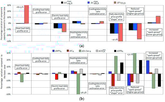
Figure 4.
Percentage variation (compared to the base case) of components’ capacities and economic, energetic and environmental results, for the eight examined types of estimation errors: (a) Capacity of the CHP unit, the absorption chiller and the Thermal Energy Storage; (b) Net Present Value, Investment Cost, Energy Saving, CO2 emissions and Simple Payback time.
According to Equation (6), the energy saving is the difference between the fuel that would be consumed by a “separate production” process, Ftrad, and the fuel consumed by the cogeneration system (including the consumption by eventual auxiliary/backup boilers), keeping into account the additional (or saved) emissions in centralized power plants due to the amounts of electricity bought from (or sold to) the public grid. Actually, the expression formulated in Equation (6) differs from the “Primary Energy Saving” index proposed by the Directive 2004/8/EC and adopted in all the member states of European Union to assess the efficient cogeneration systems. However, the preference for the formula proposed in Equation (6) is justified by the different objective pursued in this section, i.e., quantifying the energy saving achieved, rather than “qualifying” the cogeneration unit as efficient or not; this point is clarified more in details in Appendix A. As evident in Figure 4b, the energy saving and, to some extent, also the CO2 emissions reduction are primarily influenced by the factors that influence the economic viability, like the shape of the daily price profiles and the Spark Spread. Also, the heating to power ratio influences the achievable energy and CO2 emissions savings, due to the very different emission factors per kWh of electricity and heat [39]. Conversely, these energetic and environmental results are moderately influenced by the daily load profiles and the cooling to power ratio.
Although the above graphs provide some quantitative information about the influence of the examined types of estimation errors on the design and operational results of building CHP/CHCP systems, they are scarcely illustrative of the actual modifications induced in the optimized CHCP solution. A more intuitive interpretation of results may be offered by the punctual analysis of the annual energy flows obtained for the optimized solution. For this purpose, the “graphical analysis” instrument provided by the optimization tool can be very useful; it is shown in Figure 5, with reference to the optimized annual energy flows obtained for the base case.
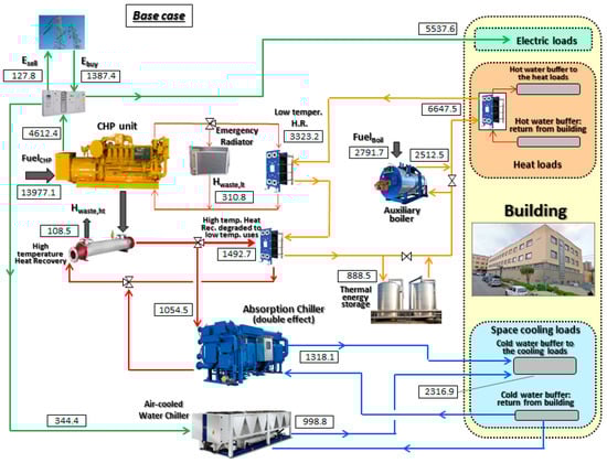
Figure 5.
Optimized energy flows (MWh), obtained for the “base case” and cumulated on annual basis, for the building CHCP system.
All the energy flows are accumulated on an annual basis and expressed in MWh. It may be observed that, in the base case, the heat recovered by the CHP unit supplies more than 60% of the annual heat load, while the remaining fraction is provided by a backup boiler. As concerns the space cooling requests, almost 57% of the annual load is supplied by the double effect absorption chiller, the rest being covered by the air-cooled vapour compression unit. Surplus electricity production occurs only for a limited number of hours, being only 127.8 MWh electricity supplied to the grid; conversely, the CHP unit often produces less electricity than required, and the grid-connected system purchases 1387.4 MWh electricity per year from the grid.
Once that a clear view of the optimal solution has been obtained in terms of annual energy flows, the results obtained for the eight scenarios accounting for estimation errors are presented in Figure 6a–h. In the figures, for a more intuitive interpretation, the values that have increased (compared to the corresponding values for the “base case”, presented in Figure 5) are shown in blue, while those that have decreased are shown in red. The values that have observed the most relevant deviations are also highlighted by using a bold dashed line. It may be observed that:
- -
- In the three scenarios developed by imposing modifications in the daily heat, cooling and electric load profiles, all the annual energy flows observe quite low deviations from the corresponding values observed in the base case. This result again testifies that the adoption of daily “standard” load profiles in order to distribute, on hourly basis, any consumption data eventually available at aggregate monthly or weekly basis is not a critical step in the analysis. Then, the creation of such standard load profiles does not deserve particular efforts, being not necessary to extrapolate very reliable curves;
- -
- The scenarios that assume major changes in the heating to electric and the cooling to electric loads, observe dramatic reductions in the energy supply by the backup units (respectively, the boiler in the former scenario, see Figure 6d, and the vapour compression chiller in the latter one, see Figure 6e), while the heat or cooling supply by the CHP unit and by the absorption chiller are scarcely influenced. An easy interpretation for this result may be given: as both these scenarios assume the same reference prices as the base case, it is evident that in a certain number of hours the combined power and heat/cooling production achieves relevant margins of profitability, and in such hours the optimal load level of the aforementioned units remains unmodified (regardless of the hourly heat to power or heat to cooling load ratio);
- -
- A modification in the shape of the daily electricity price profile induces a dramatic change in the energy balance with the grid. Compared to the results achieved in the base case, when the modified price profile is adopted the amount of energy sold to the grid significantly reduces and, conversely, the purchased electricity increases by a factor 1.65;
- -
- Major changes in the energy exchange with the grid are also observed for the two scenarios obtained for the higher and the lower value of the Spark Spread. Differently than in the previous case, however, the changes imposed in the CHP/CHCP profitability here induces, as a first effect, a dramatic change in the energy production by the CHP unit. The changes in the energy balance with the grid is only a secondary effect, provoked by the changes in the CHP electricity. This result is also confirmed by the much higher (lower) contribution given by the backup components, i.e., the boiler and the vapour compression chiller, for the scenario assuming a lower (higher) value of the Spark Spread.
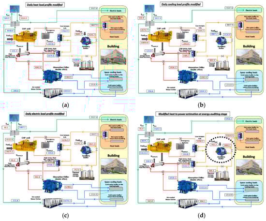
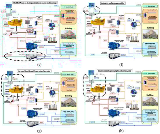
Figure 6.
Optimized energy flows (MWh), cumulated on annual basis, for the eight scenarios based on the different types of estimation errors: (a) Daily heat load profile; (b) Daily cooling load profile; (c) Daily electric load profile; (d) Heat to electricity ratio in the winter season; (e) Cooling to electricity ratio in the summer season; (f) Shape of the daily price profile; (g) Increased Spark Spread; (h) Decreased Spark Spread.
4.2. Results for Scenarios Including Different Simultaneous Estimation Errors
In the previous subsection the influence of each estimation error on the results achieved by CHCP optimization was discussed. However, in general the analyst will incur in several simultaneous estimation errors; it is worthwhile analysing the magnitude of the distortions induced in the optimization results by different possible combinations of the proposed estimation errors. In this subsection, it is initially done by examining some graphs similar to those presented in Section 4.1. In Figure 7a,b the changes induced in the optimal components’ size and the economic, energetic and environmental results by different combinations of estimation errors are presented; these two subfigures refer to the scenarios assuming the same values of Spark Spread as the base case. In Figure 7c,d the changes observed for the same combination of estimation errors are presented, imposing at meantime a deviation in the Spark Spread (25% lower than in the base case). From a rapid analysis of the graphs shown in Figure 7, it may be observed that:
- -
- The trends show a sort of linearity, in the sense that in presence of several simultaneous estimation errors, the effects induced on the optimal size of components and on the operational results are quite close to the sum of the effects induced, separately, by each effect. This is evident when comparing the first set of data in Figure 7a (case “Simultaneous error in all the daily load profiles”) with the first three sets of data in Figure 4a. Then, there is no “amplificative effect” of each possible estimation error on the effects induced by the other ones;
- -
- The effect induced by estimation error in the Spark Spread seems someway dominant compared to the effects induced by the other errors. For instance, in Figure 7d it may be observed that whatever the combination of errors related with the energy loads and the shape of daily electricity price profiles, the lower margins of profitability guaranteed in case of a lower Spark Spread imply a significant negative deviation of the Net Present Value and an increase in the Simple Payback Time, compared to the base case.
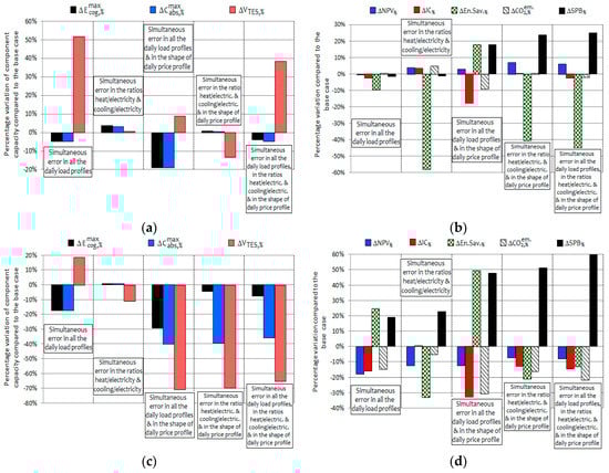
Figure 7.
Percentage variation (compared to base case) for scenarios with simultaneous estimation errors, in terms of: (a) components’ capacities, for SS equal to the base case; (b) Economic and energo-environmental results, for SS equal to the base case; (c) components’ capacities, for SS lower than in the base case; (d) economic and energo-environmental results, for SS lower than in the base case.
Once realised the effects induced by the simultaneous presence of all the examined estimation errors on the optimal plant design and on the economic and energo-environmental results, let us investigate more in details the changes induced in the optimal plant operation.
In Figure 8a–c and Figure 9a–e the operational results are shown for two consecutive days in the winter and in the summer period, respectively. The electricity purchase and selling price in the same days are also shown in the same figures, to allow for a joint interpretation of the observed trends.
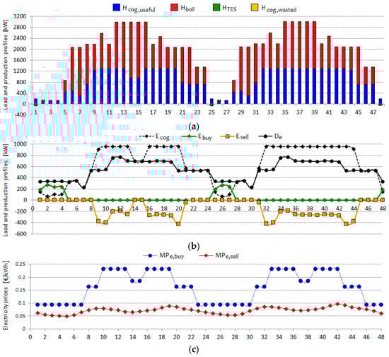
Figure 8.
Hourly operational results and energy prices for the base case, in two consecutive days in the winter period: (a) Heat balance; (b) Electricity balance and exchange with the grid; (c) Energy price profiles.
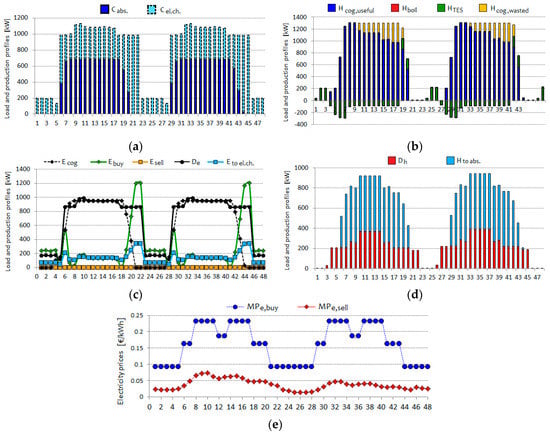
Figure 9.
Hourly operational results and energy prices for the base case, in two consecutive days in the summer period: (a) Cooling load balance; (b) Heat balance; (c) Electricity balance and exchange with the grid; (d) Heat uses; (e) Energy price profiles.
From a rapid analysis of the trends, we may observe that in the base case:
- -
- the CHP unit operates at almost full load for most of the daytime hours, which coincide with the energy price peaks;
- -
- the heat recovery from the engine approximately covers half of the heat demand during winter days. The TES is not used and no heat is wasted. During winter days, the produced electricity is always sufficient to supply the building loads, and some surplus electricity is sold to the grid during peak hours;
- -
- during summer days, the absorption chiller supplies more than 65% of the cooling load. The boiler never operates, since some surplus heat is produced and stored, with moderate amounts being wasted through hot gases and the emergency radiator. In summer no surplus electricity is produced nor sold; conversely, when the energy prices go down during the evening, the engine is switched off and significant amounts of electricity are purchased from the grid. Finally, looking at the heat uses (see Figure 9d), more than half of the heat demand is related with “indirect heat uses”, i.e., to supply the absorption chiller.
Let us now analyse the detailed results as concerns the optimized operation of the CHCP system in a completely different case, i.e., assuming that all the possible estimation errors simultaneously occur, including the Spark Spread that is assumed 25% lower than in the base case. The results are shown in Figure 10a–c and Figure 11a–e.
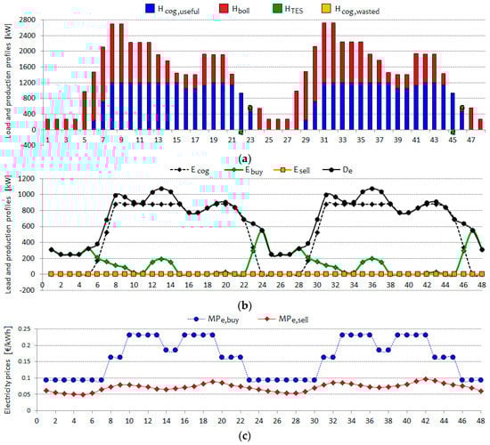
Figure 10.
Hourly operational results and energy prices for the case accounting simultaneously for all the examined estimation errors, including a lower value of the Spark Spread, in two consecutive days in the winter period: (a) Heat balance; (b) Electricity balance and exchange with the grid; (c) Energy price profiles.
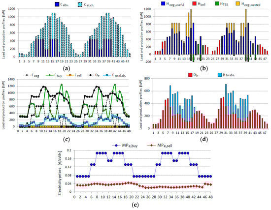
Figure 11.
Hourly operational results and energy prices for the case accounting simultaneously for all the examined estimation errors, including a lower value of the Spark Spread, in two consecutive summer days: (a) Cooling load balance; (b) Heat balance; (c) Electricity balance and exchange with the grid; (d) Heat uses; (e) Energy price profiles.
From a comparison between the corresponding trends, i.e., comparing the results in Figure 10a–c with those presented in Figure 8a–c and the results in Figure 11a–e with those presented in Figure 9a–e, several differences may be observed:
- -
- In the winter period, the optimal plant operation observes only slight changes, mainly related with the operation of the backup boiler which must now supply additional heat to follow a different daily load profile. Conversely, major modifications are observed as concerns the electricity balance: differently than in the base case, in the “modified scenario” the system never produces surplus electricity to be sold to the grid, while low amounts of energy are purchased during off-peak hours. An interpretation for this last trend is intuitive: due to the reduced price peaks during peak hours (related with the “flat” daily energy sell price profile assumed in the modified scenario), operating the CHP unit during peak hours so as to produce surplus electricity to be sold is no longer convenient. As concerns the role of the Thermal Energy Storage, in the modified scenario it provides an almost null contribute to the heat balance, exactly like in the base case. Also, the optimal operation in the modified scenario does not assume any amount of heat to be wasted, exactly as observed in the base case;
- -
- More articulate analyses are needed for the summer case, where the differences between the optimal operation obtained for the base case (see Figure 9a–e) and the modified scenario (see Figure 11a–e) are more complex. First of all, let us compare the CHP electricity production rates presented in Figure 9c and Figure 11c: it may be observed that while in the base case the CHP unit was operated at full load continuously for all the daytime hours, in the modified scenario the optimal operation of the CHP unit is much more discontinuous. Provided that the tool assumes as infeasible any prime mover operating condition with too frequent start-up/shut-down cycles, an interpretation for such an irregular operation may be given. Due to the low margins of profitability, related with the low Spark Spread and with the intrinsically lower economic convenience of combined cooling and power product in summer (compared to the heating and power production in winter), the optimal operation in the modified scenario must ensure that: (i) the energy outputs from the CHP unit are entirely used to supply a useful demand; (ii) the electricity production is self-consumed, so that each kWh of produced electricity generates an “avoided cost” MPe,buy, rather than a revenue MPe,sell (with MPe,sell much lower than MPe,buy). Also, in the modified scenario the absorption chiller supplies a much lower fraction of the cooling demand, compared to the base case.
4.3. Conceptual Achievements of the Proposed Study
The different results achieved in the proposed analysis are here harmonically summarised, in order to provide to energy analysts involved in the optimization of building CHCP systems a clear view of the possible risks related with the uncertain parameters. The following points emerged:
- The definition of daily load profiles, in terms of curve “shape”, is not a critical phase and could consequently be paid a moderate effort when conducting the energy audit of an existing building. Indeed, eventual estimation errors concerning daily load profiles will lead to minor errors in sizing the CHP unit and the absorption chiller, with slightly more significant deviations as concerns the optimal size of the heat storage. Also the economic, energetic and environmental results are scarcely sensitive to the assumed heat, cooling and electric load profiles;
- In the analysis of energy loads for existing buildings, when data on the electricity consumption for lighting and appliances and those related with HVAC systems are grouped together (as usual in the energy bills), eventual errors occurring in the allocation of these two kinds of “direct” and “indirect” electricity uses also lead to moderate changes in the optimal CHCP solution. Only in terms of avoided CO2 emissions, eventual estimation error can lead to significant under- or over-estimation due to the different emission factors per kWh of heat, cooling and electricity;
- Erroneous prediction, over the plant life cycle, of the “shape” of daily energy price profiles may induce to rather relevant changes in the optimal size of the main plant components and in the economic and energo-environmental results. This conclusion is someway intuitive, since the economic attractiveness of combined heating, cooling and power production increases whenever most of the energy loads occur during “peak hours”, i.e., hours characterized by higher energy prices;
The Spark Spread, or the average ratio between electricity and fuel prices, resulted the most critical parameter to assess the CHCP viability and converge toward reliable optimal design and operation strategies. Then, in any case the analyst should take into consideration the possibility to conduct sensitivity analyses, exploring the possible changes in the optimal values of decision variables and objective functions in case of (i) more favourable for CHCP applications (Spark Spread values higher than expected); or (ii) less favourable scenarios (Spark Spread values lower than expected).
5. Conclusions
In this paper a novel approach to deal with energy load and price uncertainty in the optimization of building CHCP systems was proposed. Rather than adopting stochastic programming, a deterministic Mixed Integer Linear Programming tool was used and iteratively applied to a number of properly defined scenarios. The study does not follow the typical approaches of “sensitivity analysis”, which often assume some generic ranges of variability for specific variables; conversely, referring to a “base case” scenario for a hotel building, a particular set of “modified scenarios” was designed, conceived in order to reflect the most common errors occurring in the energy load evaluation or in the price forecasts. Particular attention was paid to errors related with the “shape” of energy load and price profiles, with the ratio between heating/cooling and electric loads and with the so-called Spark Spread. The analysis revealed that some specific errors, namely those involving the daily energy load profiles, moderately influence the optimal CHCP solution, both in terms of component sizing and economic and energo-environmental results. On the contrary, the daily shape of energy price profiles might significant influence the optimal plant operation. Finally, the Spark Spread, i.e., the ratio between average electricity and fuel prices, plays an absolutely dominant role among the uncertain parameters, since it strongly influences the profitability of combined energy conversion systems and their optimal design and operation strategy. Then, energy analysts should always conduct accurate sensitivity analysis for different values of this parameter, in order to limit the risks of CHCP investments.
Author Contributions
A.P. conceived the whole work, coordinating the research activity and developing all the conceptual bases for the implementation of the study. R.G. implemented the code of the deterministic optimization tool. P.C., F.C. and D.P. supported the research activity, contributing to implement the sensitivity analyses.
Conflicts of Interest
The authors declare no conflict of interest.
Abbreviations and Symbols
| C | Cooling |
| D | Demand or load (kW) |
| DHW | Domestic Hot Water |
| E | Electricity |
| En.Sav. | Energy Saving |
| F | Fuel |
| H | Heat |
| Itot | Total investment cost |
| LHV | Low Heat Value (kJ/Nm3 and kJ/kg, respectively for gaseous and liquid fuels) |
| MP | Market Price (€/kWh or €/Nm3, respectively for electricity and gaseous fuels) |
| Nhours | Number of hours used as temporal basis for the optimization |
| NPV | Net Present Value |
| PHR | Power to Heat Ratio |
| Ref Eη | Reference efficiency for the separate production of electricity |
| SS | Spark Spread |
| STORi | Stored Thermal energy at the beginning of a generic time step “i” |
| V | Volume (m3) |
| Greek letters | |
| δ | Boolean 0–1 variable at plant synthesis level |
| η | Efficiency |
| Subscripts | |
| abs | Absorption chiller |
| boil | Backup boiler |
| cog | Related to the operation of the cogeneration unit |
| TES | Thermal Energy Storage |
| trad | Traditional plant, producing separately electricity, heat and/or cooling |
| Acronyms | |
| CHCP | Combiner Heat, Cooling and Power |
| CHP | Combined Heat and Power, also used to indicate “efficient cogeneration” according to European Directive |
| COP | Coefficient of Performance |
| FEL | Following the Electric Load |
| FTL | Following the Thermal Load |
| HVAC | Heating, Ventilating and Air-Conditioning |
| MILP | Mixed Integer Linear Programming |
| MINLP | Mixed Integer NonLinear Programming |
| PGU | Power Generation Unit |
Appendix A
The expression formulated in Equation (6) to evaluate the primary energy saving differs from the formulas proposed by the Directive 2004/8/EC, and it is worthwhile justifying the introduction of this expression. In the Annex II to the Directive, a Primary Energy Saving index is defined as follows:
where:
and Ref Eη and Ref Hη represent the reference efficiencies for the separate production of electricity and heat, respectively [40]. For natural gas-fuelled units, we have Ref Eη = 0.525 and Ref Hη = 0.9. The parameters ECHP, HCHP and FCHP are calculated on the basis of well established rules. For a reciprocate engine-based cogeneration plant, the following expressions apply:
The annual operation of the CHP unit, which consumes an amount of fuel “Fcog” and produces the amounts of electricity and useful heat “Ecog” and “Hcog” respectively, is decomposed into two “virtual sub-units”, one conceived as operating in efficient cogeneration (subscript “CHP”), the other one conceived as a virtual power-only unit (subscript “nonCHP”). Equations (A4)–(A8) provide the expressions used to size these sub-units. The threshold efficiency ηthreshold is imposed equal to 0.75 for ICEs-based cogeneration plants.
As an applicative example, in Figure A1 and Figure A2 the decomposition of two cogeneration units are illustrated, referring to the following data:
It may be observed that according to Equations (A4)–(A8), when decomposing the two units into their corresponding virtual “CHP” and “nonCHP” subunits:
- -
- the plant achieving a higher efficiency is decomposed into a large CHP subunit and a very small nonCHP one;
- -
- the plant achieving a lower energy efficiency is decomposed into two CHP and nonCHP subunits with comparable “sizes”.
When looking at the Primary Energy Saving index presented by Equation (A1), being the expression applied to the CHP subunit only, both the examined plants achieve a same PES%:
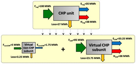
Figure A1.
Decomposition into virtual “CHP” and “nonCHP” subunits for an ICE-based cogeneration plant achieving a 73% energy efficiency.
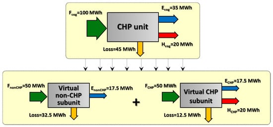
Figure A2.
Decomposition into virtual “CHP” and “nonCHP” subunits for an ICE-based cogeneration plant achieving a 55% energy efficiency.
Then, the PES index formulated by the Directive is evidently not adequate to measure the positive effects achieved by a CHP plant, due to its formulation as a dimensionless parameter. However, once assessed the CHP subunit as “high efficiency cogeneration”, a second step of the analysis (not discussed in the Directive, but included in national legislation acts implementing energy saving calculations for white certificates) quantitatively defines the energy saving as follows:
Differently than Equation (A1), this expression quantifies in energy units (MWh) the savings achieved by the CHP subunit, and thus discriminates between the two cases “a” and “b” presented before. Let us implement the PES calculation for the above two cases:
The current legislation correctly recognizes a higher energy saving to the plant achieving the higher efficiency. However, the above approach coherent with the Directive 2004/8/EC has some evident limits, since it focuses the attention on the CHP sub-unit only, disregarding the effects of the nonCHP subunit.
Contrariwise, the Energy Saving expression formulated in this paper (see Equation (6)) is coherent with the traditional concept of energy saving to be calculated as difference between the energy consumption of a reference separate production mix of technologies and the examined cogeneration plant to produce the same amounts of useful outputs. For the examined cases “a” and “b”, and in the simplifying assumption to have no energy exchanges with the grid (Esell = 0 and Ebuy = 0), Equation (6) gives:
The En.Sav. expression correctly identifies that the plant operating with a 73% total energy efficiency produces a positive energy saving compared to the separate production option, while the plant operating with a 55% total efficiency actually consumes more primary energy saving than the reference separate production technologies. In simplewords, while the legislative framework depicted by the Directive 2005/8/EC has the merit to provide a harmonized and clear framework to calculate energy savings, it has the limit not to properly account for context variables (by assuming fixed reference efficiencies for the separate production units) and for the total operation of the cogeneration unit (since the “nonCHP” operation si totally disregarded).
As the analysis presented in Section 4 is aimed at quantifying properly the externalities related with the operation of the CHP unit, and not at quantifying the way it complies with the provisions of the CHP Directive, it seems convenient to calculate the energy saving by Equation (6).
References
- Angrisani, G.; Canelli, M.; Roselli, C.; Sasso, M. Microcogeneration in buildings with low energy demand in load sharing application. Energy Convers. Manag. 2015, 100, 78–89. [Google Scholar] [CrossRef]
- Siler-Evans, K.; Granger Morgan, M.; Lima Azevedo, I. Distributed cogeneration for commercial buildings: Can we make the economics work? Energy Policy 2012, 42, 580–590. [Google Scholar] [CrossRef]
- Sanaye, S.; Khakpaay, N. Simultaneous use of MRM (maximum rectangle method) and optimization methods in determining nominal capacity of gas engines in CCHP (combined cooling, heating and power) systems. Energy 2014, 72, 145–158. [Google Scholar] [CrossRef]
- Cardona, E.; Piacentino, A. A methodology for sizing a trigeneration plant in Mediterranean areas. Appl. Therm. Eng. 2003, 23, 1665–1680. [Google Scholar] [CrossRef]
- Wang, J.J.; Bai, H.; Jing, Y.Y.; Zhang, J.L. Economic Analysis and Optimization Design of a Solar Combined Cooling Heating and Power System in Different Operation Strategies. In Proceedings of the 7th IEEE Conference on Industrial Electronics and Applications (ICIEA), Singapore, 18–20 July 2012; pp. 108–112.
- Mauser, I.; Müller, J.; Allerding, F.; Schmeck, H. Adaptive building energy management with multiple commodities and flexible evolutionary optimization. Renew. Energy 2016, 87, 911–921. [Google Scholar] [CrossRef]
- Anvari, S.; Taghavifar, H.; Khoshbakhti Saray, R.; Khalilarya, S.; Jafarmada, S. Implementation of ANN on CCHP system to predict trigeneration performance with consideration of various operative factors. Energy Convers. Manag. 2015, 101, 503–514. [Google Scholar] [CrossRef]
- Rong, A.; Lahdelma, R. An efficient linear programming model and optimization algorithm for trigeneration. Appl. Energy 2005, 82, 40–63. [Google Scholar] [CrossRef]
- Andiappan, V.; Ng, K.S.D. Synthesis of tri-generation systems: Technology selection, sizing and redundancy allocation based on operational strategy. Comput. Chem. Eng. 2016, 91, 380–391. [Google Scholar] [CrossRef]
- Arcuri, P.; Beraldi, P.; Florio, G.; Fragiacomo, P. Optimal design of a small size trigeneration plant in civil users: A MINLP (Mixed Integer Non Linear Programming Model). Energy 2015, 80, 628–641. [Google Scholar] [CrossRef]
- Morari, M. Flexibility and resiliency of process systems. Comput. Chem. Eng. 1983, 7, 423–438. [Google Scholar] [CrossRef]
- Larsson, T.; Wene, C.O. Developing strategies for robust energy systems. I: Methodology. Int. J. Energy Res. 1993, 17, 503–513. [Google Scholar] [CrossRef]
- Lai, S.M.; Hui, C.W. Feasibility and flexibility for a trigeneration system. Energy 2009, 34, 1693–1704. [Google Scholar] [CrossRef]
- Lai, S.M.; Hui, C.W. Integration of trigeneration system and thermal storage under demand uncertainties. Appl. Energy 2010, 87, 2868–2880. [Google Scholar] [CrossRef]
- Gamou, S.; Yokoyama, R.; Ito, K. Optimal unit sizing of cogeneration systems in consideration of uncertain energy demands as continuous random variables. Energy Convers. Manag. 2002, 43, 1349–1361. [Google Scholar] [CrossRef]
- Gamou, S.; Yokoyama, R.; Ito, K. Optimal sizing of cogeneration systems under the toleration for shortage of energy supply. Int. J. Energy Res. 2000, 24, 61–75. [Google Scholar] [CrossRef]
- Hu, M.; Cho, H. A probability constrained multi-objective optimization model for CCHP system operation decision support. Appl. Energy 2014, 116, 230–242. [Google Scholar] [CrossRef]
- Ersoz, I.; Colak, U. Combined cooling, heat and power planning under uncertainty. Energy 2016, 109, 1016–1025. [Google Scholar] [CrossRef]
- Li, C.Z.; Shi, Y.M.; Huang, X.H. Sensitivity analysis of energy demands on performance of CCHP system. Energy Convers. Manag. 2008, 49, 3491–3497. [Google Scholar] [CrossRef]
- Li, C.Z.; Shi, Y.M.; Liu, S.; Zheng, Z.L.; Liu, Y.C. Uncertain programming of building cooling heating and power (BCHP) system based on Monte-Carlo method. Energy Build. 2010, 42, 1369–1375. [Google Scholar] [CrossRef]
- Smith, A.; Luck, R.; Mago, P.J. Analysis of a combined cooling, heating and power system model under different operating strategies with input and model data uncertainty. Energy Build. 2010, 42, 2231–2240. [Google Scholar] [CrossRef]
- Akbari, K.; Nasiri, M.M.; Jolai, F.; Ghaderi, S.F. Optimal investment and unit sixing of distributed Energy systems under uncertainty: A robust optimization approach. Energy Build. 2014, 85, 275–286. [Google Scholar] [CrossRef]
- Wang, L.; Singh, C. Stochastic combined heat and power dispatch based on multi-objective particle swarm optimization. Int. J. Electr. Power 2008, 30, 226–234. [Google Scholar] [CrossRef]
- Carvalho, M.; Lozano, M.A.; Ramos, J.; Serra, L.M. Synthesis of trigeneration systems: Sensitivity analyses and resilience. Sci. World J. 2013, 2013, 604752. [Google Scholar] [CrossRef] [PubMed]
- Carpaneto, E.; Chicco, G.; Mancarella, P.; Russo, A. Cogeneration planning under uncertainty. Part I: Multiple time frame approach. Appl. Energy 2011, 88, 1059–1067. [Google Scholar] [CrossRef]
- Carpaneto, E.; Chicco, G.; Mancarella, P.; Russo, A. Cogeneration planning under uncertainty. Part II: Decision theory-based assessment of planning alternatives. Appl. Energy 2011, 88, 1075–1083. [Google Scholar] [CrossRef]
- Ortiga, J.; Bruno, J.C.; Coronas, A. Selection of typical days for the characterisation of energy demand in cogeneration and trigeneration optimisation models for buildings. Energy Convers. Manag. 2011, 52, 1934–1942. [Google Scholar] [CrossRef]
- Piacentino, A.; Barbaro, C. A comprehensive tool for efficient design and operation of polygeneration-based energy μgrids serving a cluster of buildings. Part II: Analysis of the applicative potential. Appl. Energy 2013, 111, 1222–1238. [Google Scholar] [CrossRef]
- Piacentino, A.; Barbaro, C.; Cardona, F.; Gallea, R.; Cardona, E. A comprehensive tool for efficient design and operation of polygeneration-based energy μgrids serving a cluster of buildings. Part I: Description of the method. Appl. Energy 2013, 111, 1204–1221. [Google Scholar] [CrossRef]
- LINDO API 8.0 User Manual; LINDO System, Inc.: Chicago, IL, USA, 2013.
- Cardona, E.; Piacentino, A. DABASI—WWW Promotion of Energy Savings by CHCP Plants, Database and Evaluation. Final Report; Project Financed within the EU SAVE Programme, Contract No. 4.1031/Z/02-060; Project Consortium: Bruxelles, Belgium, 2005. [Google Scholar]
- Environmental Protection Agency e Combined Heat and Power Partnership Program, Report “Technology Characterization: Reciprocating Engines”. Available online: http://www.epa.gov/chp/documents/catalog_chptech_reciprocating_engines.pdf (accessed on 10 February 2014).
- Directive 2004/8/EC of the European Parliament and of the Council of 11 February 2004 on the promotion of cogeneration based on a useful heat demand in the internal energy market and amending Directive 92/42/EEC. Off. J. Eur. Union 2004, 52, 50–60.
- Cardona, E.; Culotta, S. CHOSE—Energy Saving by Combined Heat, Cooling and Power Plants in the Hotel Sector. Final Report; Project Financed within the SAVE II Programme, Contract No. XVII/4.1031/Z/98-036; Project Consortium: Bruxelles, Belgium, 2001. [Google Scholar]
- Gestore dei Mercati Energetici. Available online: http://www.mercatoelettrico.org/It/Download/DatiStorici.aspx (accessed on 27 September 2016).
- Angrisani, G.; Akisawa, A.; Marrasso, E.; Roselli, C.; Sasso, M. Performance assessment of cogeneration and trigeneration systems for small scale applications. Energy Convers. Manag. 2016, 125, 194–208. [Google Scholar] [CrossRef]
- Kavvadias, K.C. Energy price spread as a driving force for combined generation investments: A view on Europe. Energy 2016, 115, 1632–1639. [Google Scholar] [CrossRef]
- Smith, A.D.; Fumo, N.; Mago, P.J. Spark spread e a screening parameter for combined heating and power systems. Appl. Energy 2011, 88, 1494–1499. [Google Scholar] [CrossRef]
- Chicco, G.; Mancarella, P. Assessment of the greenhouse gas emissions from cogeneration and trigeneration systems. Part I: Models and indicators. Energy 2008, 33, 410–417. [Google Scholar] [CrossRef]
- European Commission. Commission Decision establishing harmonized efficiency reference values for separate production of electricity and heat in application of Directive 2004/8/EC. Off. J. Eur. Union 2007, 32, 183–188. [Google Scholar]
© 2016 by the authors; licensee MDPI, Basel, Switzerland. This article is an open access article distributed under the terms and conditions of the Creative Commons Attribution (CC-BY) license (http://creativecommons.org/licenses/by/4.0/).