
Modeling and Forecasting Electricity Demand in Azerbaijan Using Cointegration Techniques

Abstract
:1. Introduction
2. Discussion of Previous Electricity Demand Studies
2.1. Previous Electricity Demand Studies in Resource-Rich Small Open Developing Economies
2.2. Previous Azerbaijan Electricity Demand Studies
3. Electricity Demand Function Specification and Data
3.1. Per Capita Electricity Demand Function
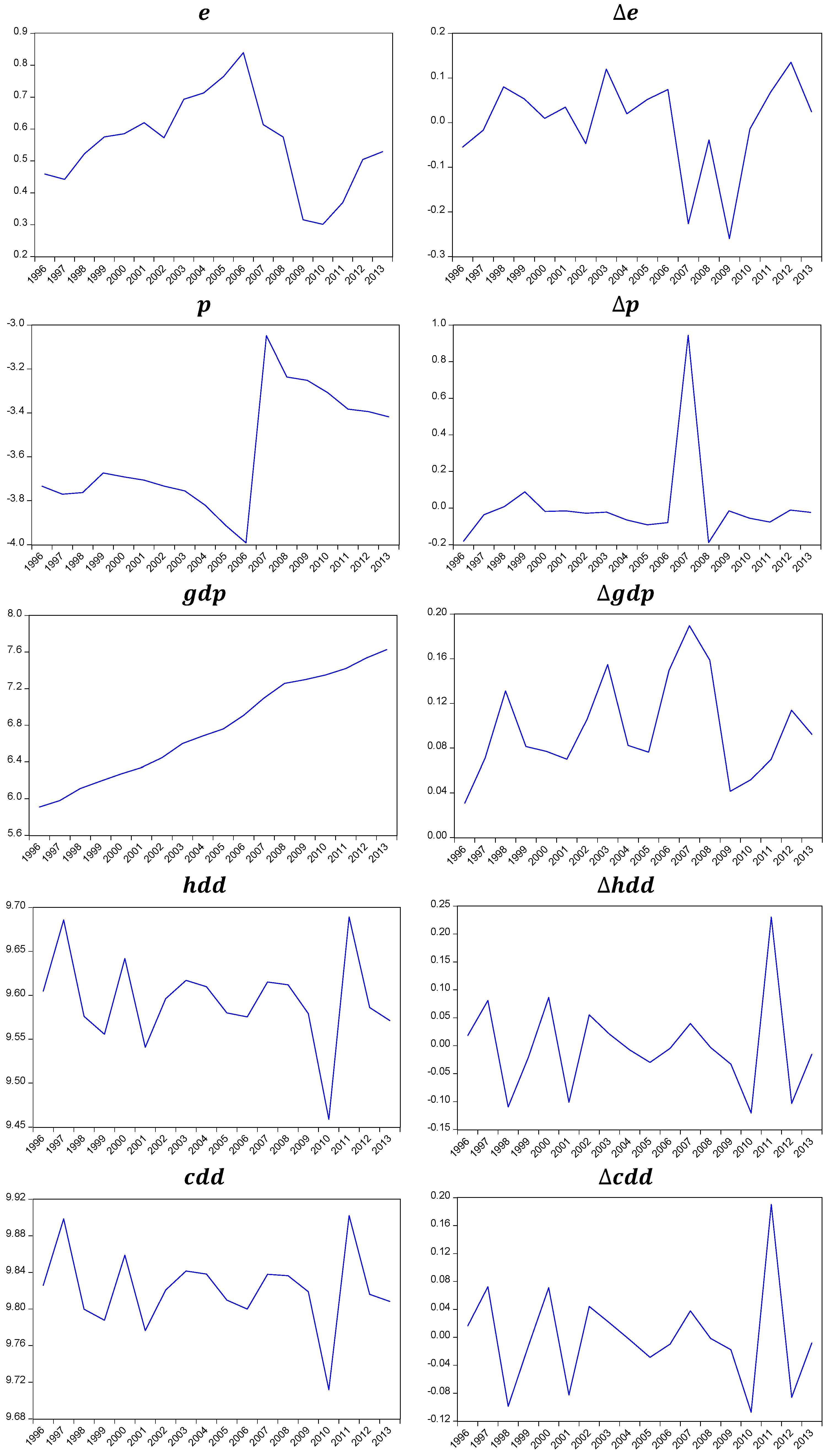
3.2. Data
- is electricity consumption per capita. This is equal to total final electricity consumption in TWh divided by population in millions. The total final electricity consumption data are collected from the International Energy Agency Database in Mtoe and then converted to TWh in order to be consistent with the electricity price [8]. Population data comes from the World Bank Database [4].
- is the real electricity price. Nominal retail electricity prices in Azerbaijani New Manat (AZN) are administratively set by the government (being the same for the industrial, residential, and commercial sectors) and are collected from the various Statistical Yearbooks of the State Statistical Committee of the Republic of Azerbaijan [9]. The real electricity prices are in 2005 AZN, found by deflating the nominal prices by the Consumer Price Index (CPI), 2005 = 100 collected from [9].
- is real Non-oil GDP per capita. This is calculated by deflating nominal Non-oil GDP in million AZN by the CPI, 2005 = 100 and then dividing by population in millions. Nominal Non-oil GDP is retrieved from [9].
- is real total GDP per capita. This is calculated in a similar way to GDP—nominal total GDP in million AZN is deflated by the CPI, 2005 = 100 and then divided by population in millions. Nominal total GDP is retrieved from [9].
- and are heating degree-days and cooling degree-days, respectively. These are summary variables of weather conditions that are considered given they might influence electricity demand. For HDD the reference temperature is 18 °C. For CDD the reference temperature is 21 °C. Both HDD and CDD come from the [46] database, where population-weighted degree-days were constructed for just under 150 countries for the period 1948 to 2013. The weather variables from [46] are calculated using a sophisticated degree-days methodology by addressing issues such as, limited geographical availability, temporal and spatial aggregation, the lack of accounting for various climatic factors, and the restrictive use of a singular reference temperature.
4. Cointegration Methodologies and Estimated Models
4.1. Methodologies
4.1.1. Unit Root Test
4.1.2. Different Cointegration Methods
The Johansen Cointegration Method
Small Sample Bias Correction in the Johansen Method
ARDLBT Method
Small Sample Bias Correction in ARDLBT Approach
EG Approaches
- (i)
- For the first step, estimate a regression equation of the non-stationary variables that are integrated in the same order (usually I(1)):where, and are the variables that are integrated in the same order; and are the coefficients to be estimated; indicates the residuals; t denotes time. The residuals from Equation (5) then need to be checked for stationarity using the UR tests outlined above. It is important to note that as [55] inter alia discus, the [83] critical values have to be used instead of [84]. If, from the test, the calculated residuals, , are found to be stationary, then it can be concluded that the variables in Equation (5) are cointegrated, the estimation results are not spurious, and can therefore be considered as a long-run relationship.
- (ii)
- The second step of the EG procedure involves estimating the short-run ECM, which is explained in the next section.
4.1.3. Error Correction Model with the General to Specific Modeling Strategy
4.2. Results
4.3. Discussion of the Estimation Results
5. Projections of Future Paths of the Electricity Demand
5.1. Methodology
5.2. Forecast Assumptions
5.3. Forecast Scenarios and Discussion
6. Summary and Conclusions
- What is the best cointegration technique for modeling per capita electricity demand in Azerbaijan?Given that for all five cointegration methods considered for modeling per capita electricity demand in Azerbaijan passed the appropriate diagnostic tests, choosing the “best” is very difficult. That said the Johansen method is the “best” and the FMOLS method the “worst” according to a number of forecast statistics presented in Table 10—however there is very little difference between them; although the FMOLS model could be regarded as a marginal outlier given the estimated coefficients are a little different to the other four methods considered.
- What are the estimated price and income elasticities for per capita electricity demand in Azerbaijan?The estimated electricity demand across the five methods vary very little. The estimated short- and long-run price elasticities range from −0.3 to −0.4 and −0.8 to −1.0, respectively—suggesting that although the response to a real electricity price change is inelastic, it is relatively high, being close to unity in the long run. Whereas, the estimated short- and long-run income elasticities range from 0.4 to 0.7 and from 0.1 to 0.2—which is also inelastic in both the short and the long run, but somewhat lower (in absolute terms) than the price elasticity in the long run.
- What do the future scenarios suggest for the development of electricity demand in Azerbaijan through to 2025?Using the estimated ECM models for all five cointegration methods, coupled with assumptions about the relevant drivers of electricity demand, the Business as Usual scenario suggests that Azerbaijan electricity demand in 2025 would be something in the order of 19½ to 21 TWh; thus illustrating an average increase of about 0.6% per annum over the period from 2013 to 2025. Of course, different assumptions about the drivers suggest different demand in the future with the highest predicted electricity demand in 2025 being about 45½ TWh according to the “high” scenario or as low as about 9 TWh according to the “low” scenario.
Acknowledgments
Author Contributions
Conflicts of Interest
References
- Filippini, M.; Hunt, L.C. Measurement of energy efficiency based on economic foundations. Energy Econ. 2015, 52, S5–S16. [Google Scholar] [CrossRef]
- Enerdata. 2016. Available online: http://www.enerdata.net/enerdatauk/knowledge/subscriptions/database/ (accessed on 10 May 2016).
- Hasanov, F.C. Dutch Disease and the Azerbaijan Economy. J. Communist Post-Communist Stud. 2013, 4, 463–480. [Google Scholar] [CrossRef]
- World Bank. Word Development Indicators. 2016. Available online: http://www.worldbank.org (accessed on 10 May 2016).
- Energy Charter Secretariat. In Depth Review of the Energy Efficiency Policy of Azerbaijan. 2013. Available online: http://www.energycharter.org/fileadmin/DocumentsMedia/IDEER/IDEER-Azerbaijan_2013_en.pdf (accessed on 25 September 2016).
- Energy Charter Secretariat. Follow-UP IN-DEPTH Review of the Investment Climate and Market Structure in the Energy Sector. 2011. Available online: http://www.energycharter.org/fileadmin/DocumentsMedia/ICMS/ICMS-Azerbaijan_2011_en.pdf (accessed on 25 September 2016).
- Ministry of Industry and Energy of Azerbaijan. 2012. Available online: http://www.minenergy.gov.az/db/2011_senaye_tehlil.pdf (accessed on 25 September 2016).
- International Energy Agency. Energy Statistics. Available online: www.iea.org (accessed on 10 May 2016).
- State Agency of Statistics of Azerbaijan. Available online: http://www.astat.org (accessed on 6 July 2016).
- Opitz, P.; Kharazyan, A.; Pasoyan, A.; Gurbanov, M.; Margvelashvili, M. Sustainable Energy Pathways in the South Caucasus: Opportunities for Development and Political Choices; South Caucasus Regional Office of the Heinrich Boell Foundation: Tbilisi, Georgia, 2015. [Google Scholar]
- Azerenerji Joint Stock Company. Electricity Forecast Report; Azerenerji: Baku, Azerbaijan, 2009.
- Azerenerji Joint Stock Company. Electricity Forecast Report; Azerenerji: Baku, Azerbaijan, 2013.
- Fichtner. Update of the Power Sector Master Plan of Azerbaijan 2013—2025; Fichtner: Stuttgart, Germany, 2013. [Google Scholar]
- Mercados. Azerenerji Generation and Transmission Master Plan 2010–2025; Fichtner: Stuttgart, Germany, 2010. [Google Scholar]
- Japan International Cooperation Agency, Tokyo Electric Power Services Co. Study for Electric Power Sector in Azerbaijan; Japan International Cooperation Agency (JICA): Tokyo, Japan; Tokyo Electric Power Services Co. (TEPSCO): Tokyo, Japan, 2013. [Google Scholar]
- Squalli, J. Electricity consumption and economic growth: Bounds and causality analyses of OPEC members. Energy Econ. 2007, 29, 1192–1205. [Google Scholar] [CrossRef]
- Narayan, P.K.; Smyth, R. Multivariate Granger causality between electricity consumption, exports and GDP: Evidence from a panel of Middle Eastern countries. Energy Policy 2009, 37, 229–236. [Google Scholar] [CrossRef]
- Chang, Y.; Choi, Y.; Kim, C.S.; Miller, J.I.; Park, J.Y. Disentangling Temporal Patterns in Elasticities: A Functional Coefficient Panel Analysis of Electricity Demand. Energy Econ. 2016, in press. [Google Scholar] [CrossRef]
- Eltony, M.N. The Sectoral Demand for Electricity in Kuwait. OPEC Rev. 1995, 19, 37–44. [Google Scholar] [CrossRef]
- Al-Faris, A.R.F. The demand for electricity in the GCC countries. Energy Policy 2002, 30, 117–124. [Google Scholar] [CrossRef]
- Klytchnikova, I. Methodology and Estimation of the Welfare Impact of Energy Reforms on Households in Azerbaijan. Ph.D. Thesis, University of Maryland, Gollege Park, MD, USA, 2006. [Google Scholar]
- Al-Sahlawi, M.A. Forecasting the Demand for Electricity in Saudi Arabia. Energy J. 1990, 11, 119–126. [Google Scholar] [CrossRef]
- Eltony, M.N.; Yousuf, H.M. The Structure of Demand for Electricity in the Gulf Cooperation Council Countries. J. Energy Dev. 1993, 18, 213–221. [Google Scholar]
- Eltony, M.N.; Asraul, H. A Cointegrating Relationship in the Demand for Energy: The Case of Electricity in Kuwait. J. Energy Dev. 1997, 21, 293–301. [Google Scholar]
- Diabi, A. The Demand for Electric Energy in Saudi Arabia: An Empirical Investigation. OPEC Rev. 1998, 22, 13–29. [Google Scholar] [CrossRef]
- Al-Sahlawi, M.A. Electricity Planning with Demand Estimation and Forecasting in Saudi Arabia. Energy Stud. Rev. 1999, 9, 82–88. [Google Scholar]
- Askari, A. Estimation of electricity demand for residential sector and its price and income elasticities. J. Barnameh Va Budjeh 2002, 63, 103. (In Farsi) [Google Scholar]
- Amini Fard, A.; Estedlal, S. Estimation of residential demand for electricity in Iran, evidence from a cointegration approach. In Proceedings of the 18th International Power System Conference, Tehran, Iran, 18–20 October 2003. (In Farsi)
- Atakhanova, Z.; Howie, P. Electricity demand in Kazakhstan. Energy Policy 2007, 35, 3729–3743. [Google Scholar] [CrossRef]
- Eltony, M.N.; Al-Awadhi, M.A. The commercial sector demand for energy in Kuwait. OPEC Rev. 2007, 31, 17–26. [Google Scholar] [CrossRef]
- Eltony, M.N.; Al-Awadhi, M.A. Residential energy demand: A case study of Kuwait. OPEC Rev. 2007, 31, 159–168. [Google Scholar] [CrossRef]
- Pourazarm, E.; Cooray, A.V. Estimating and forecasting residential electricity demand in Iran. Econ. Model. 2013, 35, 546–558. [Google Scholar] [CrossRef]
- Atalla, T.N.; Hunt, L.C. Modelling residential electricity demand in the GCC countries. Energy Econ. 2016, 59, 149–158. [Google Scholar] [CrossRef]
- Bildirici, M.E.; Kayikci, F. Economic growth and electricity consumption in former Soviet Republics. Energy Econ. 2012, 34, 747–753. [Google Scholar] [CrossRef]
- International Monetary Fund. World Economic Outlook Database. 2014. Available online: http://www.imf.org/external/pubs/ft/weo/2014/02/weodata/index.aspx (accessed on 10 May 2016).
- Bentzen, J.; Engsted, T. Short and long run elasticities in energy demand: A cointegration approach. Energy Econ. 1993, 15, 9–16. [Google Scholar] [CrossRef]
- Silk, J.; Joutz, F. Short and long-run elasticities in US residential electricity demand: A co-integration approach. Energy Econ. 1997, 19, 493–513. [Google Scholar] [CrossRef]
- Pesaran, H.; Smith, R.P.; Akiyama, T. Energy Demand in Asian Developing Economies; Oxford University Press: Oxford, UK, 1998. [Google Scholar]
- Asafu-Adjaye, J. The relationship between energy consumption, energy prices and economic growth: Time series evidence from Asian developing countries. Energy Econ. 2000, 22, 615–625. [Google Scholar] [CrossRef]
- Hossein, A.; Gudarzi, F.Y.; Asghari, G.E. The Relationship between Energy Consumption, Energy Prices and Economic Growth: Case Study (OPEC Countries). OPEC Energy Rev. 2012, 36, 272–286. [Google Scholar] [CrossRef]
- Amarawickrama, H.A.; Hunt, L.C. Electricity demand for Sri Lanka: A time series analysis. Energy 2008, 33, 724–739. [Google Scholar] [CrossRef]
- Hunt, L.C.; Judge, G.; Ninomiya, Y. Modelling Underlying Energy Demand Trends. In Energy in a Competitive Market: Essays in Honour of Colin Robinson; Hunt, L.C., Ed.; Edward Elgar Publishing: Cheltenham, UK, 2003; Chapter 9; pp. 140–174. [Google Scholar]
- Hunt, L.C.; Judge, G.; Ninomiya, Y. Underlying trends and seasonality in UK energy demand: A sectoral analysis. Energy Econ. 2003, 25, 93–118. [Google Scholar] [CrossRef]
- Amarawickrama, H.A.; Hunt, L.C. Sri Lanka electricity supply industry: A critique of the proposed reforms. J. Energy Dev. 2005, 30, 239–278. [Google Scholar]
- Hasanov, F.C.; Bulut, C.; Suleymanov, E. Do population age groups matter in the energy use of the oil-exporting countries? Econ. Model. 2016, 54, 82–99. [Google Scholar] [CrossRef]
- Atallah, T.; Gualdi, S.; Lanza, A. Enhanced degree days for energy-related applications KAPSARC Discussion PAPER, KS_1514-DP08A. 2015. Available online: https://www.kapsarc.org/wp-content/uploads/2015/10/KS-1514-DP08A-A-global-degree-days-database-for-energy-related-applications_for-web.pdf (accessed on 1 October 2016).
- Tariff (Price) Council of Azerbaijan Republic. Available online: http://www.tariffcouncil.gov.az/?/en (accessed on 9 December 2016).
- Beenstock, M.; Goldinn, E.; Nabot, D. The demand for electricity in Israel. Energy Econ. 1999, 21, 168–183. [Google Scholar] [CrossRef]
- Harvey, A.C. Forecasting, Structural Time Series Models and the Kalman Filter; Cambridge University Press: Cambridge, UK, 1989. [Google Scholar]
- Engle, R.F.; Granger, C.J. Co-integration and Error Correction: Representation, Estimation and Testing. Econometrica 1987, 55, 251–276. [Google Scholar] [CrossRef]
- Dickey, D.; Fuller, W. Likelihood Ratio Statistics for Autoregressive Time Series with a Unit Root. Econometrica 1981, 49, 1057–1072. [Google Scholar] [CrossRef]
- Phillips, P.B.; Perron, P. Testing for Unit Roots in Time Series Regression. Biometrika 1988, 75, 335–346. [Google Scholar] [CrossRef]
- Perron, P. The Great Crash, the Oil Price Shock, and the Unit Root Hypothesis. Econometrica 1989, 57, 1361–1401. [Google Scholar] [CrossRef]
- Perron, P. Dealing with Structural Breaks. In Econometric Theory, Palgrave Handbook of Econometrics; Patterson, K., Mills, T.C., Eds.; Palgrave Macmillan: London, UK, 2006; Volume 1, pp. 278–352. [Google Scholar]
- Enders, W. Applied Econometrics Time Series; Wiley Series in Probability and Statistics; University of Alabama: Tuscaloosa, AL, USA, 2010. [Google Scholar]
- Johansen, S. Statistical analysis of cointegration vectors. J. Econ. Dyn. Control 1988, 12, 231–254. [Google Scholar] [CrossRef]
- Johansen, S.; Juselius, K. Maximum likelihood estimation and inference on cointegration with applications to the demand for money. Oxf. Bull. Econ. Stat. 1990, 52, 169–210. [Google Scholar] [CrossRef]
- Johansen, S. Testing Weak Exogeneity and the Order of Cointegration in UK Money Demand Data. J. Policy Model. 1992, 14, 313–334. [Google Scholar] [CrossRef]
- Johansen, S. Cointegration in Partial Systems and the Efficiency of Single-Equation Analysis. J. Econom. 1992, 52, 389–402. [Google Scholar] [CrossRef]
- De Brouwer, G.; Ericsson, N.R. Modeling Inflation in Australia; Research Discussion Paper 9510, International Finance Discussion Paper 530; Reserve Bank of Australia: Sydney, Australia, 1995.
- De Brouwer, G.; Ericsson, N.R. Modeling Inflation in Australia. J. Bus. Econ. Stat. 1998, 16, 433–449. [Google Scholar] [CrossRef]
- Johansen, S. A small sample correction for the test of cointegrating rank in the vector autoregressive model. Econometrica 2002, 70, 1929–1961. [Google Scholar] [CrossRef]
- Reinsel, G.C.; Ahn, S.K. Vector autoregressive models with unit roots and reduced rank structure: Estimation, likelihood ratio test, and forecasting. J. Time Ser. Anal. 1992, 13, 353–375. [Google Scholar] [CrossRef]
- Reimers, H. Comparisons of tests for multivariate cointegration. Stat. Pap. 1992, 33, 335–359. [Google Scholar] [CrossRef]
- Pesaran, M.H.; Shin, Y.; Smith, R.J. Bound Testing Approaches to the Analysis of Level Relationships. J. Appl. Econom. 2001, 16, 289–326. [Google Scholar] [CrossRef]
- Pesaran, H.M.; Shin, Y. An Autoregressive Distributed Lag Modeling Approach to Cointegration Analysis. In Econometrics and Economic Theory in the 20th Century: The Ragnar Frisch Centennial Symposium; Strom, S., Ed.; Cambridge University Press: Cambridge, UK, 1999. [Google Scholar]
- Pesaran, H.M.; Pesaran, B. Working with Microfit 4.0: Interactive Econometric Analysis; Oxford University Press: Oxford, UK, 1997. [Google Scholar]
- Narayan, P.K. An Econometric Model of Tourism Demand and a Computable General Equilibrium Analysis of the Impact of Tourism: The Case of the Fiji Islands. Ph.D. Thesis, Department of Economics, Monash University, Melbourne, Australia, 2004. [Google Scholar]
- Narayan, P.K. The Saving and Investment Nexus for China: Evidence from Cointegration Tests. Appl. Econ. 2005, 37, 1979–1990. [Google Scholar] [CrossRef]
- Stock, J.H.; Watson, M.W. A simple estimator of cointegrating vectors in higher order integrated systems. Econometrica 1993, 61, 783–820. [Google Scholar] [CrossRef]
- Saikkonen, P. Asymptotically efficient estimation of cointegrated regressions. Econom. Theory 1991, 7, 1–21. [Google Scholar] [CrossRef]
- Saikkonen, P. Estimation and testing of cointegrated systems by an autoregressive approximation. Econom. Theory 1992, 8, 1–27. [Google Scholar] [CrossRef]
- Wickens, M.R.; Breusch, T.S. Dynamic Specification, the Long-Run and the Estimation of Transformed Regression Models. Econ. J. 1988, 98, 189–205. [Google Scholar] [CrossRef]
- Park, J.Y. Canonical Cointegrating Regressions. Econometrica 1992, 60, 119–143. [Google Scholar] [CrossRef]
- Park, J.Y.; Phillips, P.B. Statistical Inference in Regressions with Integrated Processes: Part I. Econom. Theory 1988, 4, 468–497. [Google Scholar] [CrossRef]
- Phillips, P.B.; Hansen, B.E. Statistical Inference in Instrumental Variables Regression with I(1) Processes. Rev. Econ. Stud. 1990, 57, 99–125. [Google Scholar] [CrossRef]
- Phillips, P.B.; Loretan, M. Estimating Long-run Economic Equilibria. Rev. Econ. Stud. 1991, 58, 407–436. [Google Scholar] [CrossRef]
- Charemza, W.W.; Deadman, D.F. New Directions in Econometric Practice; Edward Elgar: Cheltenham, UK, 1992. [Google Scholar]
- Cuthbertson, K.; Hall, S.G.; Taylor, M.P. Applied Econometric Techniques; Simon and Schuster: New York, NY, USA; University of Michigan Press: Ann Arbor, MI, USA, 1992. [Google Scholar]
- Inder, B. Estimating Long-run Relationships in Economics. J. Econom. 1993, 57, 53–68. [Google Scholar] [CrossRef]
- Engle, R.F.; Yoo, B.S. Cointegrated Economic Time Series: An Overview with New Results. In Long-Run Economic Relationships: Readings in Cointegration; Engle, R.F., Granger, C.W.J., Eds.; Oxford University Press: New York, NY, USA, 1991. [Google Scholar]
- Utkulu, U. How to Estimate Long-Run Relationships in Economics, an Overview of Recent Development. DEÜİİBF Dergisi 1997, 12, 39–48. [Google Scholar]
- MacKinnon, J. Critical Values for Cointegration Test. In Long-Run Economic Relationships; Engle, R., Granger, C., Eds.; Oxford University Press: Oxford, UK, 1991. [Google Scholar]
- MacKinnon, J. Numerical Distribution Functions for Unit Root and Cointegration Tests. J. Appl. Econom. 1996, 11, 601–618. [Google Scholar] [CrossRef]
- Hunt, L.; Manning, N. Energy price- and income-elasticities of demand: Some estimates for the UK using the cointegration procedure. Scott. J. Political Econ. 1989, 36, 183–193. [Google Scholar] [CrossRef]
- Banerjee, A.; Dolado, J.J.; Gailbraith, J.; Hendry, D. Co-integration, Error-Correction, and the Econometric Analysis of Non-Stationary Data; Advanced Texts in Econometrics; Oxford University Press: Oxford, UK, 1986. [Google Scholar]
- Campos, J.; Ericsson, N.R.; Hendry, D.F. General-to-specific Modeling: An Overview and Selected Bibliography, Board of Governors of the Federal Reserve System, International Finance Discussion Papers, 838. 2005. Available online: http://www.federalreserve.gov/pubs/ifdp/2005/838/ifdp838.pdf (accessed on 25 September 2016). [Google Scholar]
- Ng, S.; Perron, P. Unit root test in ARMA models with data-dependent methods for the selection of the truncation lag. J. Am. Stat. Assoc. 1995, 90, 268–281. [Google Scholar] [CrossRef]
- Newey, W.; West, K. Autocovariance lag selection in covariance matrix estimation. Rev. Econ. Stud. 1994, 61, 613–653. [Google Scholar] [CrossRef]
- Rapanos, V.; Polemis, M. Energy demand and environmental taxes: The case of Greece. Energy Policy 2005, 33, 1781–1788. [Google Scholar] [CrossRef]
- Polemis, M. Modeling industrial energy demand in Greece using cointegration techniques. Energy Policy 2007, 35, 4039–4050. [Google Scholar] [CrossRef]
- Johansen, S. Likelihood-Based Inference in Cointegrated Vector Autoregressive Models; Oxford University Press: New York, NY, USA, 1995. [Google Scholar]
- MacKinnon, J.G.; Alfred, A.H.; Leo, M. Numerical distribution functions of likelihood ratio tests for cointegration. J. Appl. Econom. 1999, 14, 563–577. [Google Scholar] [CrossRef]
- Juselius, K. The Cointegrated VAR Model: Methodology and Applications; Oxford University Press: Oxford, UK, 2006. [Google Scholar]
- Hendry, D.F.; Ericsson, N.R. Understanding Economic Forecasts; MIT Press: Cambridge, MA, USA, 2001. [Google Scholar]
- Allen, P.G.; Fildes, R.A. Econometric forecasting strategies and techniques. In Principles of Forecasting: A Handbook for Researchers and Practitioners; Armstrong, J.S., Ed.; Kluwer Academic Press: Dordrecht, The Netherlands, 2001. [Google Scholar]
- Diebold, F.X. Elements of Forecasting; South-Western College Publishing: Cincinnati, OH, USA, 1988. [Google Scholar]
- Granger, C.J.; Newbold, P. Forecasting Economic Time Series, 2nd ed.; Academic Press: New York, NY, USA, 1986. [Google Scholar]
- Clements, M.P.; Hendry, D.F. Forecasting Non-Stationary Time Series; MIT Press: Cambridge, MA, USA, 1999. [Google Scholar]
- Clements, M.P.; Hendry, D.F. Economic forecasting in a changing world. Capital. Soc. 2008, 3, 1–18. [Google Scholar] [CrossRef]
- Fakulta Hospodarskej Informatiky. Available online: http://www.fhi.sk/files/katedry/kove/predmety/Prognosticke_modely/Methods_basics.pdf (accessed on 26 September 2016).
- Engle, R.F.; Yoo, B.S. Forecasting and testing in co-integrated systems. J. Econom. 1987, 35, 143–159. [Google Scholar] [CrossRef]
- Clements, M.P.; Hendry, D.F. Forecasting in cointegrated systems. J. Appl. Econom. 1995, 10, 127–146. [Google Scholar] [CrossRef]
- Armstrong, J.S. Principles of Forecasting: A Handbook for Researchers and Practitioners; Springer Science & Business Media, Business & Economics: Berlin, Germany, 2001; p. 849. [Google Scholar]
- Azerbaijan 2020: Look into the Future Concept. Available online: http://www.president.az/files/future_en.pdf (accessed on 24 July 2016).
- International Monetary Fund. IMF World Economic Outlook; IMF: Washington, DC, USA, 2013. [Google Scholar]
- International Monetary Fund. Available online: http://www.imf.org/external/np/sec/pr/2016/pr16260.htm (accessed on 26 September 2016).
- World Bank. Available online: http://www-wds.worldbank.org/external/default/WDSContentServer/WDSP/IB/2015/07/21/090224b083014397/2_0/Rendered/PDF/Azerbaijan000C0the0period0FY2016020.pdf (accessed on 26 September 2016).
- United Nations. Department of Economic and Social Affairs. Population Division. World Population Prospects, the 2015 Revision. 2016. Available online: https://esa.un.org/unpd/wpp/Download/Standard/Population/ (accessed on 24 July 2016).
- Hasanov, F.; Hasanli, K. Why had the Money Market Approach been irrelevant in explaining inflation in Azerbaijan during the rapid economic growth period. Middle East. Financ. Econ. 2011, 10, 1–11. [Google Scholar]
- Fitch. Fitch Ratings. 2016. Available online: http://azeri.press/iqtisadayyat/253557-fitch-azerbaycanda-inflyasiya-proqnozunu-yaxslasdrd--yenilenib.html (accessed on 24 July 2016).
- Asian Development Bank. Asian Development Bank Outlook 2016. Asian’s Potential Growth. 2016. Available online: http://www.adb.org/sites/default/files/publication/182221/ado2016.pdf (accessed on 24 July 2016).
- The World Bank. Economic Update: Impact of China on Europe and Central Asia. Available online: http://www-wds.worldbank.org/external/default/WDSContentServer/WDSP/IB/2016/05/03/090224b0842f1054/3_0/Rendered/PDF/The0impact0of00ope0and0Central0Asia.pdf (accessed on 26 September 2016).
- IMF. World Economic Outlook (WEO). Too Slow for Too Long. Available online: http://www.imf.org/external/pubs/ft/weo/2016/01/pdf/tblparta.pdf (accessed on 26 September 2016).


| Study | Period | Country or Region | Sector | Methodology | Income Elasticity | Price Elasticity | ||
|---|---|---|---|---|---|---|---|---|
| Short-Run | Long-Run | Short-Run | Long-Run | |||||
| Al-Sahlawi (1990) [22] | 1970–1985 | Saudi Arabia | Aggregate | OLS | 0.37 | 1.02 | Not reported | Not reported |
| Eltony and Mohammad (1993) [23] | 1975–1989 | GCC | Residential | OLS | 0.20 | 0.20 | −0.14 | −0.14 |
| Commercial | 1.12 | 2.37 | −0.20 | −0.41 | ||||
| Industrial | 0.60 | 0.89 | −0.14 | −0.20 | ||||
| Eltony (1995) [19] | 1974–1989 | Kuwait | Residential | OLS | 0.09 | 0.57 | −0.06 | −0.39 |
| Commercial | 0.11 | 1.93 | −0.13 | −2.20 | ||||
| Industrial | 0.02 | 0.13 | −0.05 | −0.27 | ||||
| Eltony and Hoque (1997) [24] | 1975–1994 | Kuwait | Aggregate | ECM | 0.57 | 0.65 | −1.09 | −1.97 |
| Commercial | 0.43 | 0.62 | −0.27 | −0.35 | ||||
| Diabi (1998) [25] | 1980–1992 | Saudi Arabia | Aggregate | OLS, GLS, MLE, CHTA and CCTA | 0.05 to 0.33 | 0.09 to 0.49 | −0.003 to −0.12 | −0.14 to 0.01 |
| Al-Sahlawi (1999) [26] | 1975–1996 | Saudi Arabia | Aggregate | OLS | 0.21 | 1.60 | −0.06 | −0.46 |
| Residential | 0.13 | 0.70 | −0.10 | −0.50 | ||||
| Industrial | 0.08 | 0.66 | No price variable included | |||||
| Al-Faris (2002) [20] | 1970–1997 | Saudi Arabia | Aggregate | Johansen cointegration | 0.05 | 1.65 | −0.04 | −1.24 |
| UAE | 0.02 | 2.52 | −0.09 | −2.43 | ||||
| Kuwait | 0.70 | 0.33 | −0.08 | −1.10 | ||||
| Oman | 0.02 | 0.79 | −0.07 | −0.82 | ||||
| Bahrain | 0.02 | 5.39 | −0.06 | −3.39 | ||||
| Qatar | 0.08 | 2.65 | −0.18 | −1.09 | ||||
| Askari (2002) [27] | 1995–1999 | Iran | Residential | GLS | 0.11 | 0.16 | −0.97 | −1.36 |
| Amini Fard and Estedlal (2003) [28] | 1967–2000 | Iran | Residential | ECM | 0.00 | 0.24 | 0.00 | −0.59 |
| Atakhanova and Howie (2007) [29] | 1994–2003 | Kazakhstan | Aggregate | Panel GMM | 0.72 | Not reported | 0.00 | Not reported |
| Industrial | 0.78 | Not reported | 0.00 | Not reported | ||||
| Services | 0.75 | Not reported | −0.12 | Not reported | ||||
| Residential | 0.12 | 0.59 | −0.22 | −1.10 | ||||
| Eltony and Al-Awadhi (2007) [30] | 1975–2003 | Kuwait | Commercial | ECM | 0.34 | 0.50 | −0.33 | −1.64 |
| Eltony and Al-Awadhi (2007) [31] | 1975–2005 | Kuwait | Residential | ECM | 0.18 | 0.31 | −0.23 | −0.56 |
| (Energy demand actually modeled, but consists predominately of electricity.) | ||||||||
| Pourazarm and Cooray (2013) [32] | 1967–2009 | Iran | Residential | ARDLBT | 0.04 (But insignificant) | 0.58 | −0.03 (But insignificant) | 0.00 |
| Atalla and Hunt (2016) [33] | 1985–2012 | Saudi Arabia | Residential | STSM | 0.00 | 0.48 | −0.10 | −0.10 |
| Oman | 0.72 | 0.86 | −0.09 | −0.10 | ||||
| Kuwait | 0.30 | 0.43 | 0.00 | 0.00 | ||||
| Bahrain | 0.00 | 0.71 | 0.00 | 0.00 | ||||
| (Qatar and UAE results are omitted since estimated equations were poorly specified.) | ||||||||
| Mean | 1.76 | 0.03 | 970.97 | 1653.42 | 14,690.97 | 18,432.05 |
| Median | 1.77 | 0.02 | 799.07 | 1125.45 | 14,563.70 | 18,378.19 |
| Maximum | 2.31 | 0.05 | 2053.05 | 3376.73 | 16,143.83 | 19,973.30 |
| Minimum | 1.35 | 0.02 | 357.23 | 397.81 | 12,821.17 | 16,511.11 |
| Standard Deviation | 0.25 | 0.01 | 551.69 | 1132.71 | 734.86 | 769.38 |
| Variable | The ADF Test | The PP Test | |||||||
|---|---|---|---|---|---|---|---|---|---|
| Test Value | C | t | None | k | Test Value | C | t | None | |
| −2.992 | x | x | 2 | −1.767 | x | x | |||
| −2.851 | x | x | 0 | −2.851 | x | x | |||
| −2.675 | x | x | 1 | −2.497 | x | x | |||
| −4.737 *** | x | 1 | −8.051 *** | x | |||||
| −5.081 *** | x | 1 | −10.460 *** | x | |||||
| −3.569 *** | x | 0 | −3.607 *** | x | |||||
| −5.109 *** | x | 0 | −5.370 *** | x | |||||
| −3.987 *** | x | 1 | −3.052 * | x | |||||
| Panel A: Serial Correlation LM Test a | |||||
| Lags | LM-Statisticb | Probability | |||
| 1 | 2.572 | 0.979 | |||
| 2 | 13.550 | 0.139 | |||
| 3 | 4.174 | 0.900 | |||
| Panel B: Normality Test b | |||||
| Statistic | d.f. | Probability | |||
| Skewness | 4.827 | 3 | 0.185 | ||
| Kurtosis | 3.366 | 3 | 0.339 | ||
| Jarque-Bera | 8.193 | 6 | 0.224 | ||
| Panel C: Heteroscedasticity Test c | |||||
| White | d.f. | Probability | |||
| Statistic | 81.226 | 78 | 0.379 | ||
| Panel D: Johansen Cointegration Test Summary | |||||
| Data Trend: | None | None | Linear | Linear | Quadratic |
| Test Type: | (a) No C and t | (b) Only C | (c) Only C | (d) C and t | (e) C and t |
| Trace: | 1 | 1 | 1 | 1 | 1 |
| Max-Eig: | 1 | 2 | 1 | 1 | 1 |
| Panel E: Johansen Cointegration Test Results for Type c | |||||
| Null Hypothesis: | r = 0 | r ≤ 1 | r ≤ 2 | ||
| λtrace | 41.065 ** | 11.049 | 0.635 | ||
| λa trace | 31.403 ** | 8.449 | 0.485 | ||
| λmax | 30.016 ** | 10.414 | 0.635 | ||
| λa max | 22.953 ** | 7.964 | 0.485 | ||
| Panel A: Statistics for Testing the Significance of a Given Variable in the Cointegrating Space a | |||
| E | p | gdp | |
| χ2 (1) | 17.774 *** | 14.688 *** | 18.714 *** |
| Panel B: Multivariate Statistics for Testing Stationarity b | |||
| E | p | gdp | |
| χ2 (2) | 22.129 *** | 29.215 *** | 26.452 *** |
| Panel C: Weak Exogeneity Test Statistics c | |||
| E | p | gdp | |
| χ2 (1) | 19.152 *** | 0.002 | 3.499 * |
| Methods | Intercept | ||
|---|---|---|---|
| Coef. (Std. Er.) | Coef. (Std. Er.) | Coef. (Std. Er.) | |
| VECM | −0.950 (0.084) *** | 0.191 (0.031) *** | −4.148 (0.562) *** |
| ARDLBT | −0.994 (0.094) *** | 0.204 (0.034) *** | −4.401 (0.536) *** |
| DOLS | −0.894 (0.078) *** | 0.174 (0.028) *** | −3.909 (0.425) *** |
| FMOLS | −0.788 (0.118) *** | 0.143 (0.052) *** | −3.264 (0.717) *** |
| CCR | −0.984 (0.145) *** | 0.207 (0.059) *** | −4.398 (0.864) *** |
| Method | Johansen | ARDLBT | DOLS | CCR | FMOLS |
|---|---|---|---|---|---|
| Panel A: The final ECM Specifications | |||||
| Regressor | Coef. (Std. Er.) | Coef. (Std. Er.) | Coef. (Std. Er.) | Coef. (Std. Er.) | Coef. (Std. Er.) |
| −0.921 (0.100) *** | - | - | - | - | |
| - | −0.879 (0.097) *** | - | - | - | |
| - | - | −0.969 (0.108) *** | - | - | |
| - | - | - | −0.892 (0.098) *** | - | |
| - | - | - | - | −1.025 (0.140) *** | |
| −0.039 (0.028) | −0.022 (0.028) | 0.026 (0.026) | −0.009 (0.027) | −0.038 (0.035) | |
| −0.367 (0.044) *** | −0.373 (0.045) *** | −0.356 (0.045) *** | −0.372 (0.045) *** | −0.324 (0.051) *** | |
| 0.328 (0.051) *** | 0.330 (0.052) *** | 0.321 (0.052) *** | 0.331 (0.053) *** | 0.295 (0.061) *** | |
| 0.483 (0.285) | 0.402 (0.283) | 0.580 (0.299) * | 0.412 (0.285) | 0.707 (0.371) * | |
| Panel B: Statistics, Residuals Diagnostics and Misspecification tests results | |||||
| 0.0331 | 0.0335 | 0.0339 | 0.0336 | 0.0403 | |
| AIC | −3.738 | −3.717 | −3.689 | −3.710 | −3.345 |
| SBC | −3.493 | −3.472 | −3.444 | −3.465 | −3.100 |
| 0.196 [0.826] | 0.258 [0.777] | 0.064 [0.939] | 0.257 [0.778] | 0.260 [0.776] | |
| 0.538 [0.475] | 0.516 [0.485] | 0.774 [0.394] | 0.420 [0.528] | 3.636 [0.077] * | |
| 0.333 [0.851] | 0.324 [0.857] | 0.405 [0.802] | 0.332 [0.851] | 0.936 [0.476] | |
| 3.957 [0.138] | 4.144 [0.126] | 2.554 [0.279] | 3.910 [0.142] | 1.259 [0.533] | |
| FFF | 0.178 [0.681] | 0.146 [0.710] | 0.426 [0.528] | 0.221 [0.647] | 2.236 [0.163] |
| Variable | Scenarios | ||
|---|---|---|---|
| “High“ Scenario | Business as Usual | “Low“ Scenario | |
| Non-oil GDP, million AZN 2005 prices | 8% growth (Based on [105]) | 4% growth (Based on projections from [108]) | 2% growth (Based on projections from [106,107]) |
| Population, millions | 1.0% growth (High Variant from [109]) | 0.7% growth (Medium Variant from [109]) | 0.5% growth (Low Variant from [109]) |
| Consumer price index, %, 2005 = 100 | 8% growth (Based on projections from [106,110,111,112,113,114]) | 4% growth (Based on average growth rate of 2009–2013) | 2% growth (Based on projections from [106,110,111,112,113,114]) |
| Electricity price, AZN per kwh | 0% growth (Based on making nominal prices unchanged) | 4% growth (Based on making real prices unchanged) | 17% increase in 2016, 34% increase in 2019 and 68% in 2022 |
| Year | Population, Millions | Non-oil GDP, Million AZN in 2005 Price | Consumer Price Index, 2005 = 100 | Electricity Price, AZN per kwh | ||||||||
|---|---|---|---|---|---|---|---|---|---|---|---|---|
| HS | BU | LS | HS | BU | LS | HS | BU | LS | HS | BU | LS | |
| 2014 | 9.54 | 9.54 | 9.54 | 20,789.71 | 20,789.71 | 20,789.71 | 185.53 | 185.53 | 185.53 | 0.06 | 0.06 | 0.06 |
| 2015 | 9.65 | 9.65 | 9.65 | 22,800.40 | 22,800.40 | 22,800.40 | 192.95 | 192.95 | 192.95 | 0.06 | 0.06 | 0.06 |
| 2016 | 9.88 | 9.87 | 9.86 | 24,624.43 | 23,712.41 | 23,256.41 | 208.39 | 200.67 | 196.81 | 0.06 | 0.06 | 0.07 |
| 2017 | 10.00 | 9.97 | 9.94 | 26,594.39 | 24,660.91 | 23,721.53 | 225.06 | 208.70 | 200.75 | 0.06 | 0.07 | 0.07 |
| 2018 | 10.12 | 10.07 | 10.02 | 28,721.94 | 25,647.35 | 24,195.97 | 243.06 | 217.05 | 204.76 | 0.06 | 0.07 | 0.07 |
| 2019 | 10.23 | 10.16 | 10.09 | 31,019.69 | 26,673.24 | 24,679.88 | 262.51 | 225.73 | 208.86 | 0.06 | 0.07 | 0.09 |
| 2020 | 10.34 | 10.24 | 10.14 | 33,501.27 | 27,740.17 | 25,173.48 | 283.51 | 234.76 | 213.04 | 0.06 | 0.07 | 0.09 |
| 2021 | 10.44 | 10.32 | 10.19 | 36,181.37 | 28,849.78 | 25,676.95 | 306.19 | 244.15 | 217.30 | 0.06 | 0.08 | 0.09 |
| 2022 | 10.53 | 10.38 | 10.23 | 39,075.88 | 30,003.77 | 26,190.49 | 330.69 | 253.91 | 221.64 | 0.06 | 0.08 | 0.16 |
| 2023 | 10.62 | 10.44 | 10.27 | 42,201.95 | 31,203.92 | 26,714.30 | 357.14 | 264.07 | 226.07 | 0.06 | 0.08 | 0.16 |
| 2024 | 10.70 | 10.50 | 10.30 | 45,578.10 | 32,452.08 | 27,248.59 | 385.71 | 274.63 | 230.60 | 0.06 | 0.09 | 0.16 |
| 2025 | 10.78 | 10.55 | 10.32 | 49,224.35 | 33,750.16 | 27,793.56 | 416.57 | 285.62 | 235.21 | 0.06 | 0.09 | 0.16 |
| Statistic | Final ECM Specifications | ||||
|---|---|---|---|---|---|
| Johansen | ARDLBT | DOLS | CCR | FMOLS | |
| Root Mean Squared Error | 0.410 ## | 0.422 | 0.417 # | 0.422 | 0.502 |
| Mean Absolute Error | 0.316 ## | 0.325 | 0.320 # | 0.327 | 0.430 |
| Mean Abs. Percent Error | 2.108 ## | 2.126 # | 2.183 | 2.147 | 2.891 |
| Theil Inequality Coefficient | 0.013536 ## | 0.013924 | 0.013785 # | 0.013910 | 0.016605 |
| Bias Proportion | 0.000210 | 0.000007 # | 0.001382 | 0.000002 ## | 0.005110 |
| Variance Proportion | 0.001463 ## | 0.011423 | 0.059960 | 0.006865 # | 0.338458 |
| Covariance Proportion | 0.998327 ## | 0.988570 | 0.938658 | 0.993133 # | 0.656431 |
| Method | Scenario | 2013 | 2015 | 2020 | 2025 |
|---|---|---|---|---|---|
| ARDLBT | HS | 15.985 | 17.390 | 27.761 | 45.542 |
| BU | 15.985 | 17.390 | 19.550 | 20.802 | |
| LS | 15.985 | 17.390 | 14.707 | 8.929 | |
| CCR | HS | 15.985 | 17.461 | 27.832 | 45.523 |
| BU | 15.985 | 17.461 | 19.626 | 20.893 | |
| LS | 15.985 | 17.461 | 14.783 | 9.032 | |
| DOLS | HS | 15.985 | 17.097 | 26.317 | 41.149 |
| BU | 15.985 | 17.097 | 18.941 | 20.069 | |
| LS | 15.985 | 17.097 | 14.514 | 9.332 | |
| FMOLS | HS | 15.985 | 16.802 | 24.798 | 36.844 |
| BU | 15.985 | 16.802 | 18.393 | 19.400 | |
| LS | 15.985 | 16.802 | 14.447 | 9.848 | |
| Johansen | HS | 15.985 | 17.270 | 27.145 | 43.608 |
| BU | 15.985 | 17.270 | 19.284 | 20.483 | |
| LS | 15.985 | 17.270 | 14.616 | 9.101 | |
| HS MAX | 15.985 | 17.461 | 27.832 | 45.542 | |
| BU MAX | 15.985 | 17.461 | 19.626 | 20.893 | |
| BU MIN | 15.985 | 16.802 | 18.393 | 19.400 | |
| LS MIN | 15.985 | 16.802 | 14.447 | 8.929 |
© 2016 by the authors; licensee MDPI, Basel, Switzerland. This article is an open access article distributed under the terms and conditions of the Creative Commons Attribution (CC-BY) license (http://creativecommons.org/licenses/by/4.0/).
Share and Cite
Hasanov, F.J.; Hunt, L.C.; Mikayilov, C.I. Modeling and Forecasting Electricity Demand in Azerbaijan Using Cointegration Techniques. Energies 2016, 9, 1045. https://doi.org/10.3390/en9121045
Hasanov FJ, Hunt LC, Mikayilov CI. Modeling and Forecasting Electricity Demand in Azerbaijan Using Cointegration Techniques. Energies. 2016; 9(12):1045. https://doi.org/10.3390/en9121045
Chicago/Turabian StyleHasanov, Fakhri J., Lester C. Hunt, and Ceyhun I. Mikayilov. 2016. "Modeling and Forecasting Electricity Demand in Azerbaijan Using Cointegration Techniques" Energies 9, no. 12: 1045. https://doi.org/10.3390/en9121045
APA StyleHasanov, F. J., Hunt, L. C., & Mikayilov, C. I. (2016). Modeling and Forecasting Electricity Demand in Azerbaijan Using Cointegration Techniques. Energies, 9(12), 1045. https://doi.org/10.3390/en9121045