Horizontal Air-Ground Heat Exchanger Performance and Humidity Simulation by Computational Fluid Dynamic Analysis

Abstract

Improving energy efficiency in buildings and promoting renewables are key objectives of European energy policies. Several technological measures are being developed to enhance the energy performance of buildings. Among these, geothermal systems present a huge potential to reduce energy consumption for mechanical ventilation and cooling, but their behavior depending on varying parameters, boundary and climatic conditions is not fully established. In this paper a horizontal air-ground heat exchanger (HAGHE) system is studied by the development of a computational fluid dynamics (CFD) model. Summer and winter conditions representative of the Mediterranean climate are analyzed to evaluate operation and thermal performance differences. A particular focus is given to humidity variations as this parameter has a major impact on indoor air quality and comfort. Results show the benefits that HAGHE systems can provide in reducing energy consumption in all seasons, in summer when free-cooling can be implemented avoiding post air treatment using heat pumps.

1. Introduction

A horizontal air-ground heat exchanger is a technical system whose principal component is an underground pipe located close to a building and connected to it. This system is able to pre-cool (in summer) or pre-heat (in winter) the air passing through it before entering a building. The air that leaves the pipe is used for ventilation and also for handling building thermal loads partially or totally.

The physical phenomenon that this system uses is based on specific geothermal properties: ground temperature is commonly higher than outdoor temperature in winter while the opposite occurs in summer. This difference in temperature makes the ground suitable for pre-heating or pre-cooling air. Normally, ground temperature remains almost constant throughout the year; its temperature profile as a function of depth depends on several factors, principally soil physical properties and climatic conditions [1].

This work concerns a thermo-fluid dynamic analysis of the operation and performance of a geothermal horizontal air-ground heat exchanger (HAGHE) under transient operating conditions. The research uses experimental and computational fluid dynamics modeling implemented in the FLUENT software (version 16.2, ANSYS Inc.: Canonsburg, PA, USA). A predominantly hot and humid climate of southern Italy, specifically the town of Otranto (Lecce), has been considered.

Other studies have been aimed at analyzing the performance of geothermal systems in different Italian climates [2] where the best convenience results for the HAGHE have been found only for cold climates. In winter re-heating the HAGHE air downstream is however necessary before supplying air in a building, while in summer indoor comfort conditions are sometimes achievable also without an active re-cooling [3]. Indeed, the goal of this work is to demonstrate that, at least in the summer season, it is possible to implement free-cooling avoiding the post-treatment with heat pumps. Nevertheless, few research investigations [4,5] have been carried out to evaluate the HAGHE energy performances as a function of the main boundary conditions, above all for Italian climates.

The implementation of ground source heat pump systems may result in primary energy consumption reduction of up to 60% compared to conventional heating and cooling systems [6,7,8,9,10,11]. This potential, considering the necessity of reducing energy consumption in buildings [12], minimizing greenhouse footprints [13] and promoting renewable energy sources [14], resulted in a significant increase of HAGHE installations in many countries in recent years [15]. An example of this trend is Greece, where the installed capacity of HAGHE systems increased more than 100% annually during the last 5 years [16]. HAGHE systems can be divided into two categories, depending on operation type, autonomous or in combination with a conventional heating or cooling system, referred to as hybrid systems [17,18,19].

In this work, the system is independent and it uses a 5 m long single pipe, a key parameter for the simulation; this type of heat exchanger is indicated for residential buildings as it allows treating a small amount of air. Such applications take advantage of the excavation made for the construction of the building, at least in part, exploiting an expansion of the excavation in order to contain costs. The pipe section chosen is circular, which is typically recommended for underground ducts as it reduces load losses and better withstands the pressure of the overlying ground. For the pipe material, polyethylene (PEX) and polypropylene (PP) have been chosen for their lower environmental impact and thermal conductivity compared to polyvinyl chloride (PVC) and metals. Particular types of materials [20,21,22], with suitable additives, are currently under study for the inlet air and condensation chambers; these zones must have a surface treatment to prevent the formation of mold caused by physical and organic agents. Many studies have been conducted [3,4,23,24,25,26,27,28,29,30,31,32,33,34,35,36,37,38,39,40,41,42,43,44,45,46,47,48,49,50,51,52,53,54,55,56,57] using a transient and implicit model based on numerical heat transfer and CFDs. These models evaluate the effects of the operating parameters (the pipe length, radius, depth, geometry and air flow rate) on thermal performance and cooling capacity of ground-air-pipe systems. It is concluded that CFD is an effective tool for predicting the behavior and performance of a wide variety of heat exchangers.

In this work a single linear pipe has been chosen, as it is a good compromise between cost and function, although different geometries have also been analysed [58]. Compared to recent studies [59], the main focus of this work is the monitoring of the humidity level to demonstrate that, at least in the summer season, it is possible to implement the free cooling avoiding the need for post-treatment with a heat pump.

During winter, a geothermal heat exchanger significantly increases the external air temperature reducing the costs for energy (Figure 1a). In summer, the external air is cooled to avoid very hot air entering the building; this is not an active cooling of the rooms (Figure 1b).

The flow rate and the cooling power of the heat exchanger heat may not be sufficient. In summer, combining the geothermal exchanger with an air post-treatment by roof-top provides a comfortable and pleasant building microclimate.

2. Model and Methods

2.1. Description of Computational Fluid Dynamic Model

Numerical simulation has been used as a calibrated tool from experimental methods for the development of studies in heat transfer and fluid mechanics, with subsequent applications in engineering design and industry. It is well known that the CFD solution includes detailed information of the flow variables at each grid. They provide numerical solutions of partial differential equations governing fluid flow and heat transfer in a discretized form. In this study, to examine the airflow and heat transfer processes in an HAGHE system, FLUENT software has been used [60]. FLUENT software is a computer program that allows the modelling of fluid flow and heat transfer in complex computational domains, following the principles of conservation and ensuring the integrity of magnitudes during processes.

In the present study, it has been assumed that air is an ideal gas and the ground is homogeneous with constant physical properties. It has been assumed that the physical properties of the pipes and ground materials do not change with temperature. Engineering materials are isotropic and homogeneous. The fundamental equations of fluid flow and heat transfer have been implemented in the analysis. The mesh, geometric modeling, physical and thermal parameters are the same as in previous research work [59]. In the present analysis, CFD simulations have been performed using a structured grid. Since there is a higher temperature gradient close to the pipe wall, the grid is designed to be denser in that area, while it is coarser farther away from it.

The main objective of the CFD analysis is to study the transient behavior of a simple HAGHE system operating in summer and winter and to evaluate its thermal performance under dynamic conditions including the presence of humidity.

2.2. Ground Tube Model Description

The model which is used to predict the ground heat transfer from a buried pipe has been developed under base assumptions, in order to ensure that the model is valid for a realistic system and not for an oversimplified one. The first assumption is that fluid flow within the pipe is hydrodynamically established. This assumption allows a single correlation to be used for any given fluid and flow regime. The next assumption is that the ground temperature around the pipe (2 m above and 2 m below the pipe, which represents the grid limits) can be calculated using the model developed by Kusuda and Achenbach [61]. This assumption allows the ground temperature to be uniform along the axial length of the grid element. The ground is homogeneous and maintains constant thermal properties. The temperature inside the pipe has been calculated by the FLUENT software using Equation (1):

$$T(Z_{depth},t_{year})=T_{mean}-T_{amp}\times \exp \left\{-Z_{depth}{\left(\frac{\mathsf{\pi }}{365{\mathsf{\alpha }}_{soil}}\right)}^{\raisebox{1ex}{$1$}\!\left/ \!\raisebox{-1ex}{$2$}\right.}\right\}\times \cos \left\{\frac{2\mathsf{\pi }}{365}\left[t_{year}-t_{shift}-\frac{Z_{depth}}{2}{\left(\frac{365}{{\mathsf{\pi }\mathsf{\alpha }}_{soil}}\right)}^{\raisebox{1ex}{$1$}\!\left/ \!\raisebox{-1ex}{$2$}\right.}\right]\right\}$$

(1)

The variables used in Equation (1) are defined in

Table 1. Constants used in Equation (1).

Symbol	Description
Tmean	Annual average surface temperature (K)
Tamp	Annual surface temperature amplitude (K)
Zdepth	Pipe burial depth (m)
αsoil	Ground thermal diffusivity (m2/day)
tyear	Simulation run time (day)
Tshift	Day of minimum surface temperature (8 February) (day)

.

The mathematical model, calibrated by using experimental data [62], follows the same assumptions: the HAGHE has a uniform cross-section area, the ground properties are isotropic, a perfect contact exists between the tube and the ground, thermal resistance due to tube thickness is negligible, air is incompressible and its thermal properties are constant, and the air is well mixed in the tube without temperature stratification.

2.3. Numerical Set-up

This study concerns a linear ground heat exchanger consisting of a cross-linked polyethylene pipe buried at three different depths (3 m, 4 m, 5 m). These three possible depths have been considered sufficient to show how performance changes with depth. The pipe has a diameter of 0.2 m. The heat exchangers have been simulated under three different ground types (λ = 1 W/(mK), λ = 2 W/(mK), λ = 3 W/(mK)). Weather data related to a climatic station, located in Otranto, have been used [63]. Different combinations of the above described parameters have been set up in the simulations to identify their effect on the system. The obtained results are related to the heat exchange in both summer and winter, the total energy balance with the surrounding ground, the influence of the heat exchanger on the ground temperature in comparison with that undisturbed by the heat exchanger. It is possible that during the shutdown of the system, when the input air flow is close to zero, the air flow may, occasionally, reverse direction; in this case a back flow total temperature has been set in the boundary conditions. In this way, the numerical code can model the back flow, providing the correct values during the system shutdown periods.

Before starting the dynamic simulations, the ground temperature above and below the pipe has to be stabilized setting steady state conditions.

3. Parametric Performance Analysis

3.1. Effect of the Depth

In Figure 2, Figure 3, Figure 4, Figure 5, Figure 6, Figure 7, Figure 8, Figure 9 and Figure 10, the effect of the pipe burial depth on the HAGHE performance is shown. Considering the system operation during the winter period (the coldest week), the graphs (Figure 2a, Figure 3a and Figure 4a) show that the outlet air temperature of the geothermal pipe follows the trend of the inlet temperature; it is almost slightly increased; therefore, the benefits in terms of pre-heating may be poor. As regards the operation of the system in the summer period (the warmest week) (Figure 2b, Figure 3b and Figure 4b), the outlet air temperature of the geothermal pipe presents a good reduction compared to the indoor temperature, despite the limited length of the pipe. Since these data concern a pipe only 5 m long, a temperature reduction of 2–3 °C is certainly indicative of the high efficiency of the geothermal heat exchanger, during summer. The effect of the burial depth pipe has no influence on outlet air temperature.

The results of the thermal flow in the winter period (Figure 5a, Figure 6a and Figure 7a) show the presence of oscillations at the exchanger, present in almost every switch on of the system. However, there are no reverse flows during operation and the system has the possibility to preheat the air inlet minimally, with a flow rate inlet air of 150 m³/h, for the whole daily operation period (the office hours) with a fan that consumes about 80–100 W under real operating conditions.

In the summer months (Figure 5b, Figure 6b and Figure 7b), the heat flow reaches significant values. During these months, the fluctuations are very limited during the period of the system operational period and the heat exchanger can pre-treat the inlet air in a very efficient way. Clearly, a smaller volumetric input flow rate, and a corresponding lower air speed, gives the possibility of a more efficient thermal exchange with the ground that results in a cooler temperature and better conditioning. The heat load of a 100 m² building with average insulation needs 1.000 kWh/year thermal load which could be met at 50% with three 20 m long pipes. Considering a burial depth of 5 m with a ground conductivity of 1 W/(mK), both in winter and summer, an improvement of heat flux is obtained.

Relative humidity is a parameter of fundamental importance in the model. Results show that in winter time (Figure 8a, Figure 9a and Figure 10a), during the period of system operation, the output air humidity of the pipe generally follows the value of the input. For this reason, to avoid air entering the indoor environment with a low moisture content, a post-treatment may be necessary to guarantee optimal conditions. Differently, in summer months (Figure 8b, Figure 9b and Figure 10b) the relative humidity is maintained constantly below 60%. The results on relative humidity together with air temperature in summer allow free-cooling by passing the heat pump.

3.2. Effect of the Thermal Conductivity

In Figure 11, Figure 12, Figure 13, Figure 14, Figure 15, Figure 16, Figure 17, Figure 18 and Figure 19, the effect of the thermal conductivity (λ_ground = 1, 2, 3 W/(mK)) on the HAGHE performance has been reported. In relation to the outlet air temperature of the geothermal pipe during winter and summer (Figure 11, Figure 12 and Figure 13), results show the same trend as the simulations of burial depth. The effect of the ground conductivity has no significant influence on outlet air temperature.

The results of the thermal flow (Figure 14, Figure 15 and Figure 16) during winter and summer periods, follow the same trend as the simulations of burial depths.

The results of relative humidity (Figure 17, Figure 18 and Figure 19) also show a similar trend obtained in the simulations of burial depth.

The best relative humidity results have been obtained for the following conditions: burial depth of 3 m and ground conductivity λ_ground of 1 W/(mK) (Figure 17); burial depth of 5 m and ground conductivity λ_ground of 2 W/(mK), both in winter and summer (Figure 18); burial depth of 3 m and ground conductivity λ_ground of 3 W/(mK) (Figure 19).

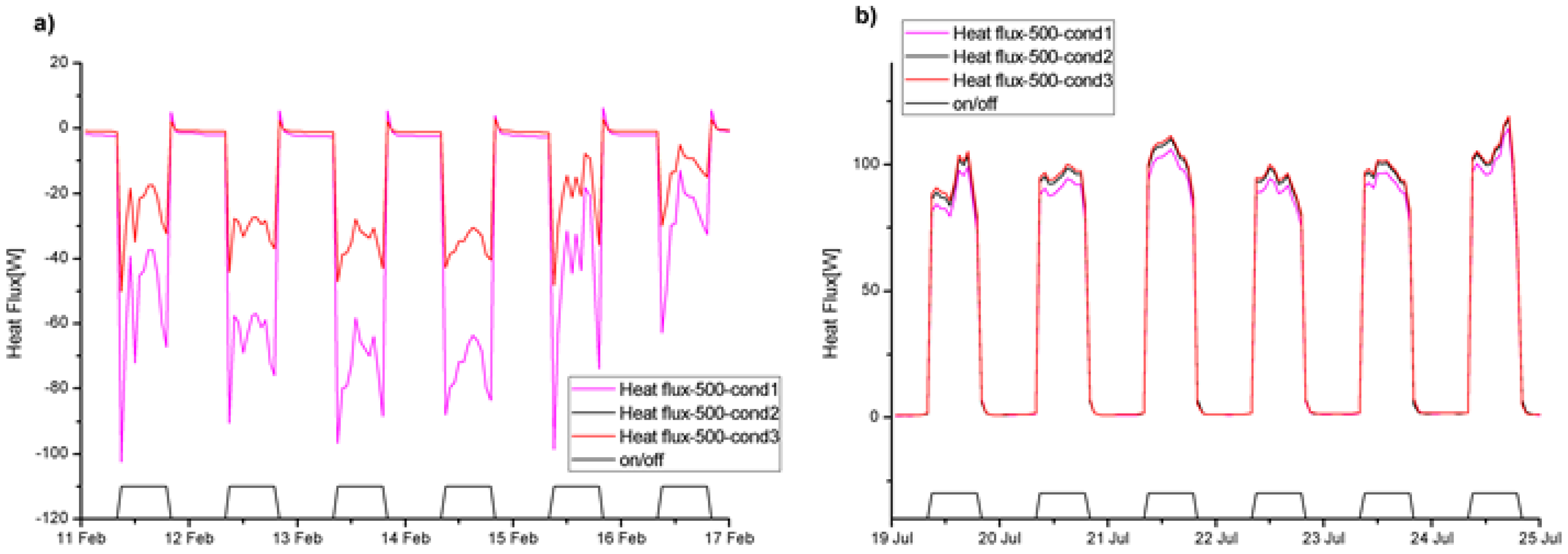
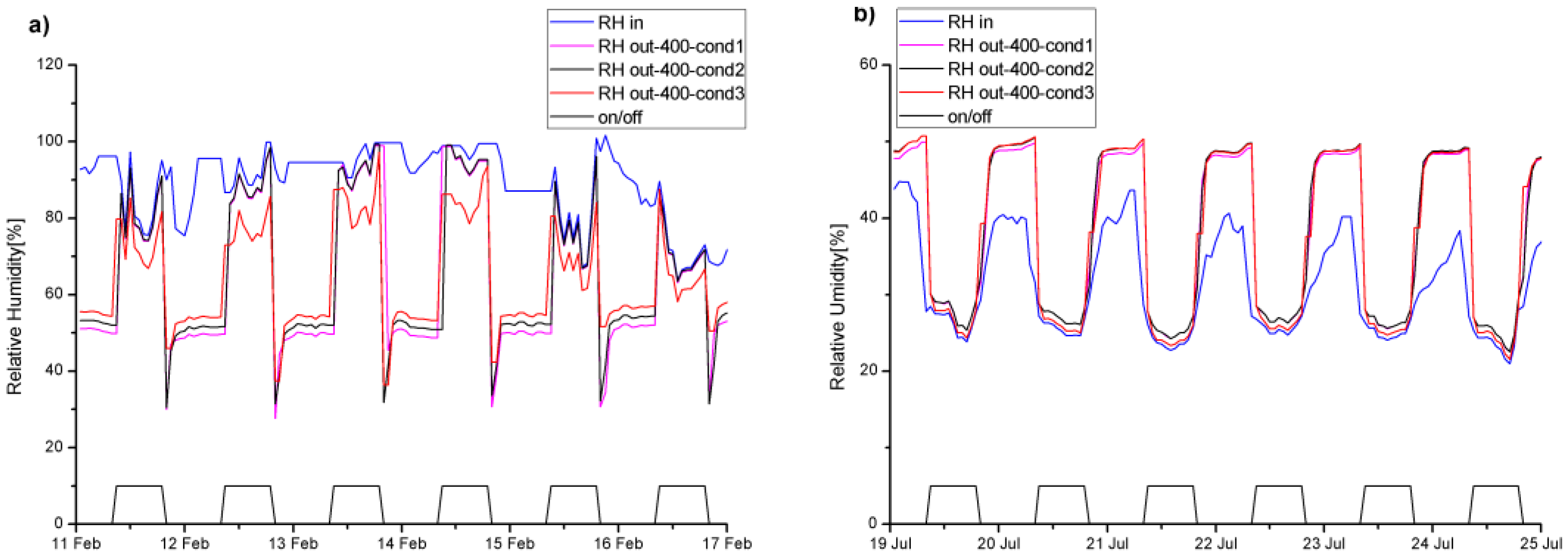
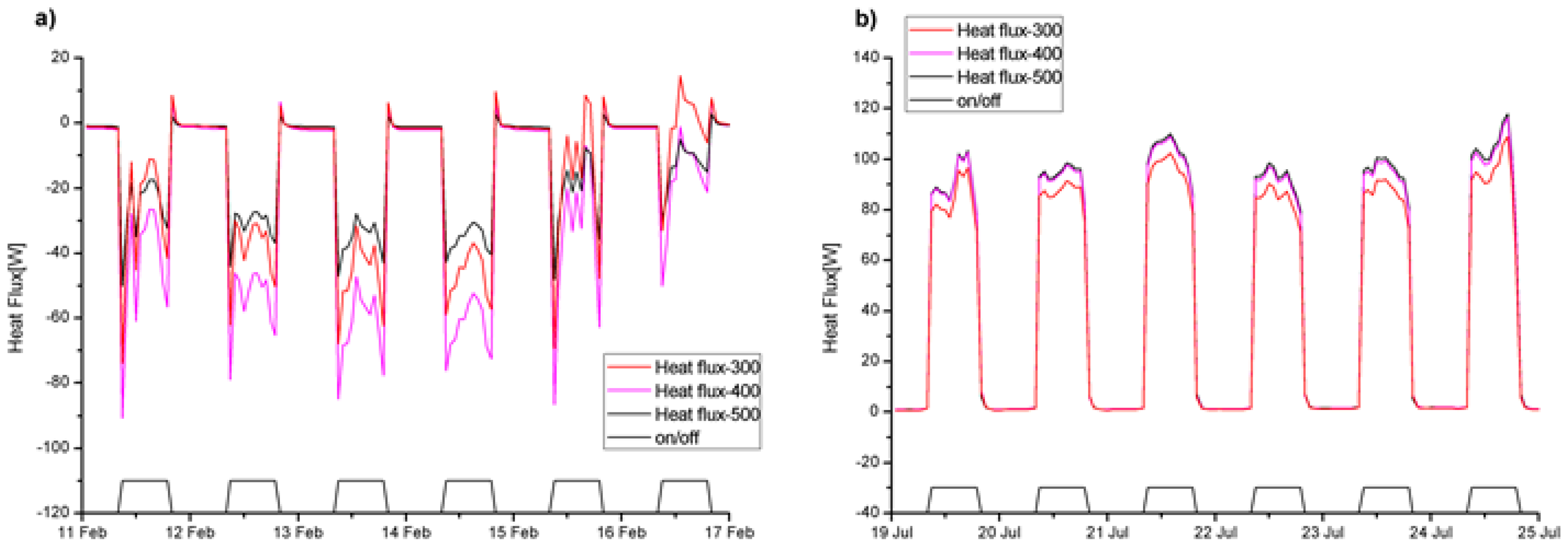
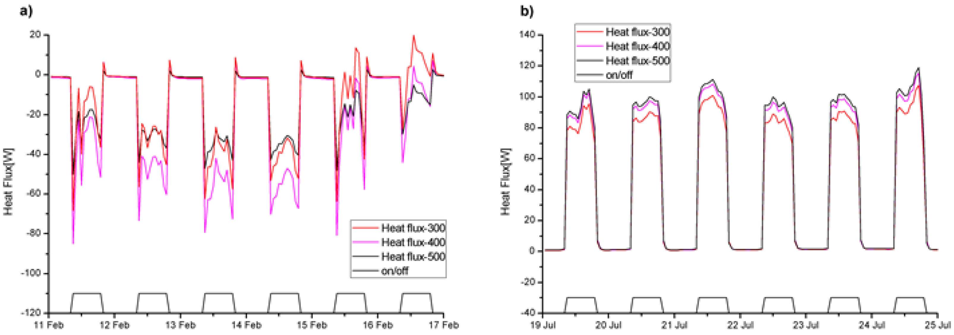
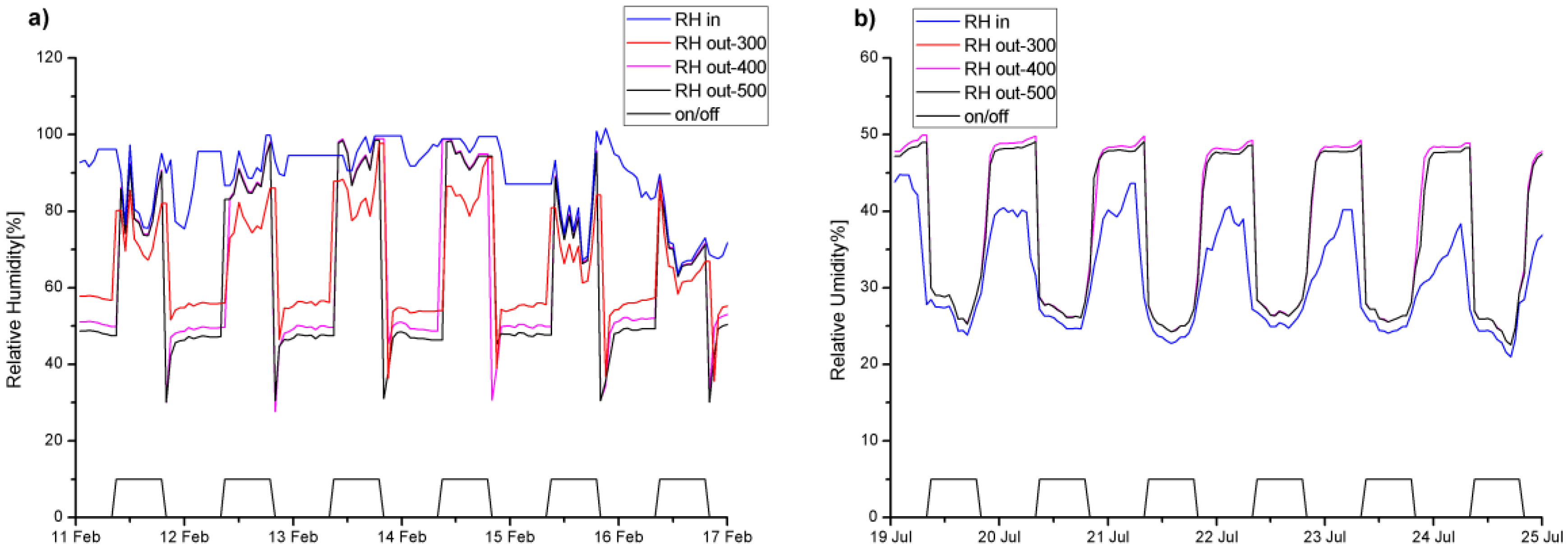
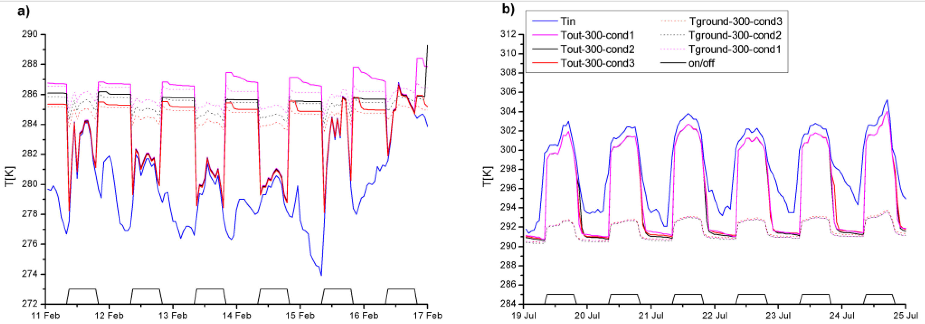
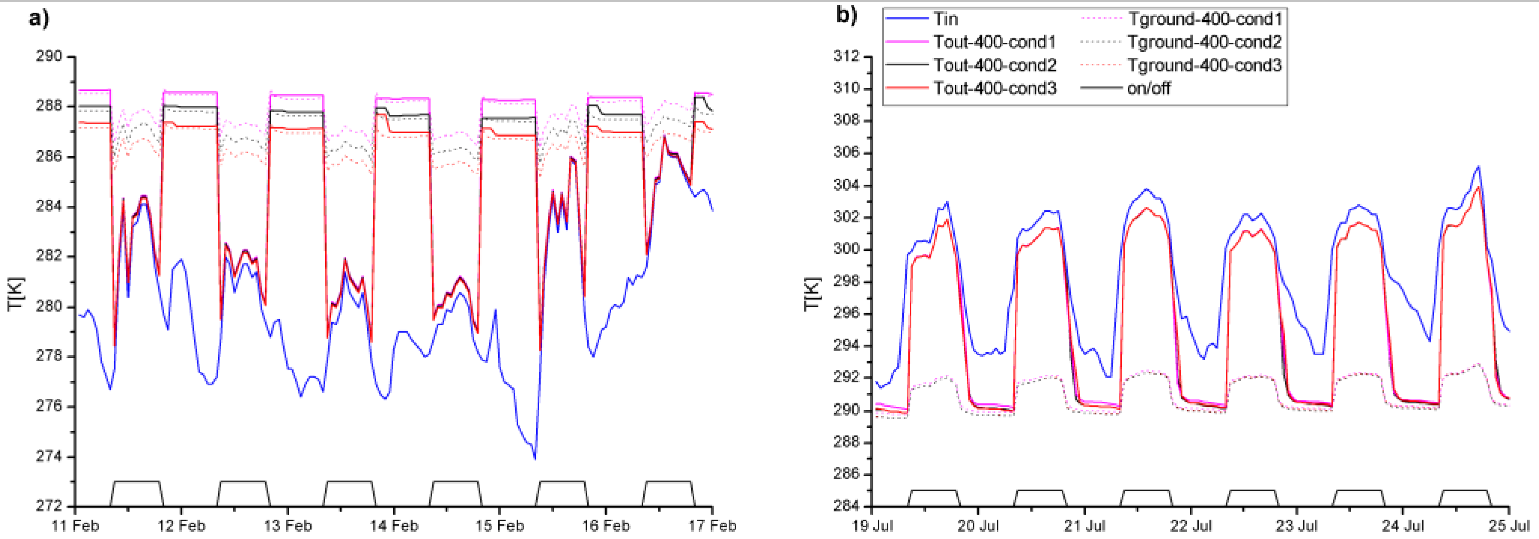
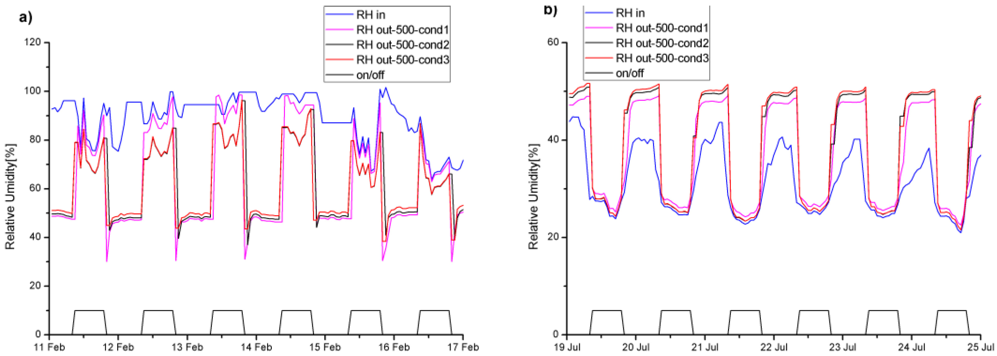
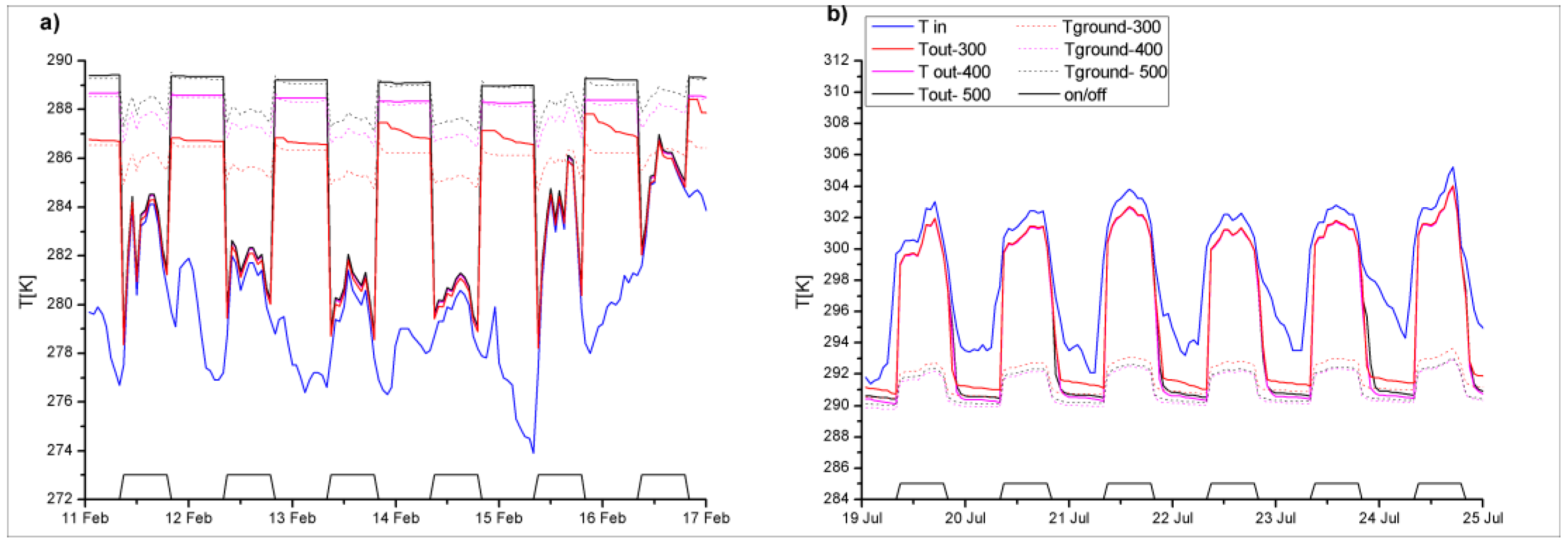
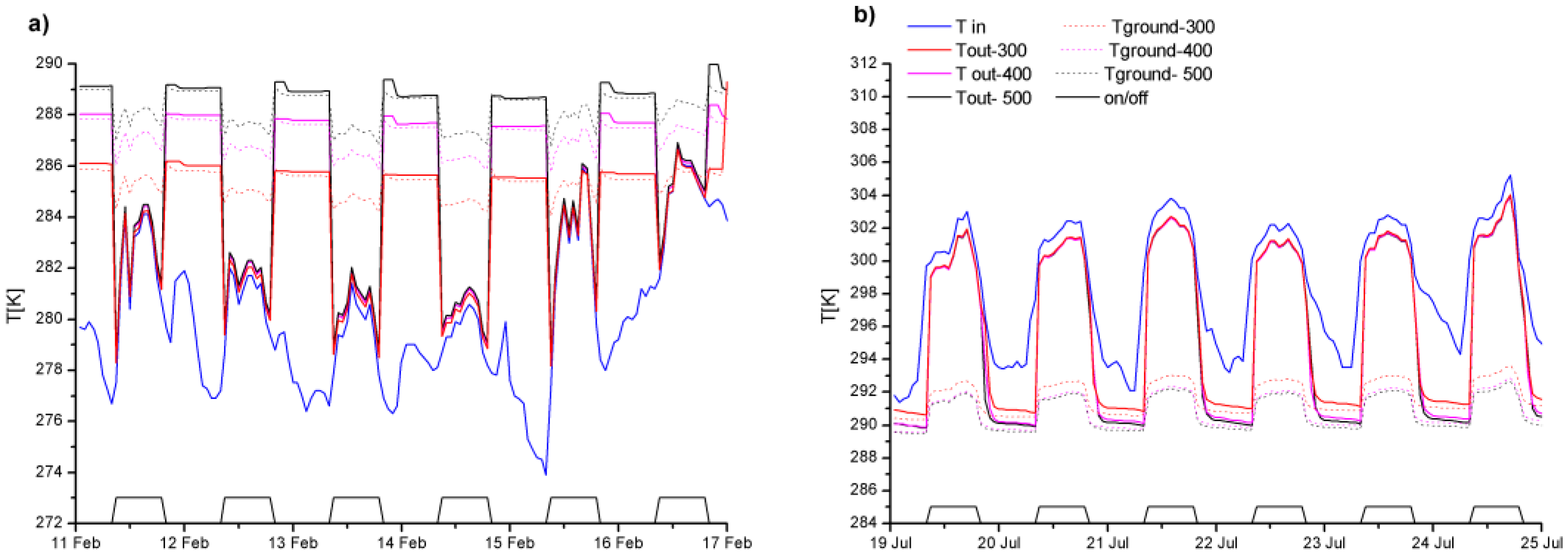
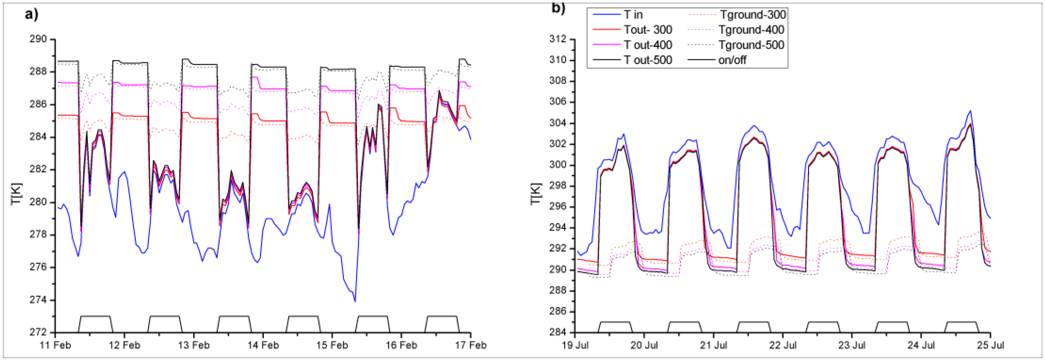
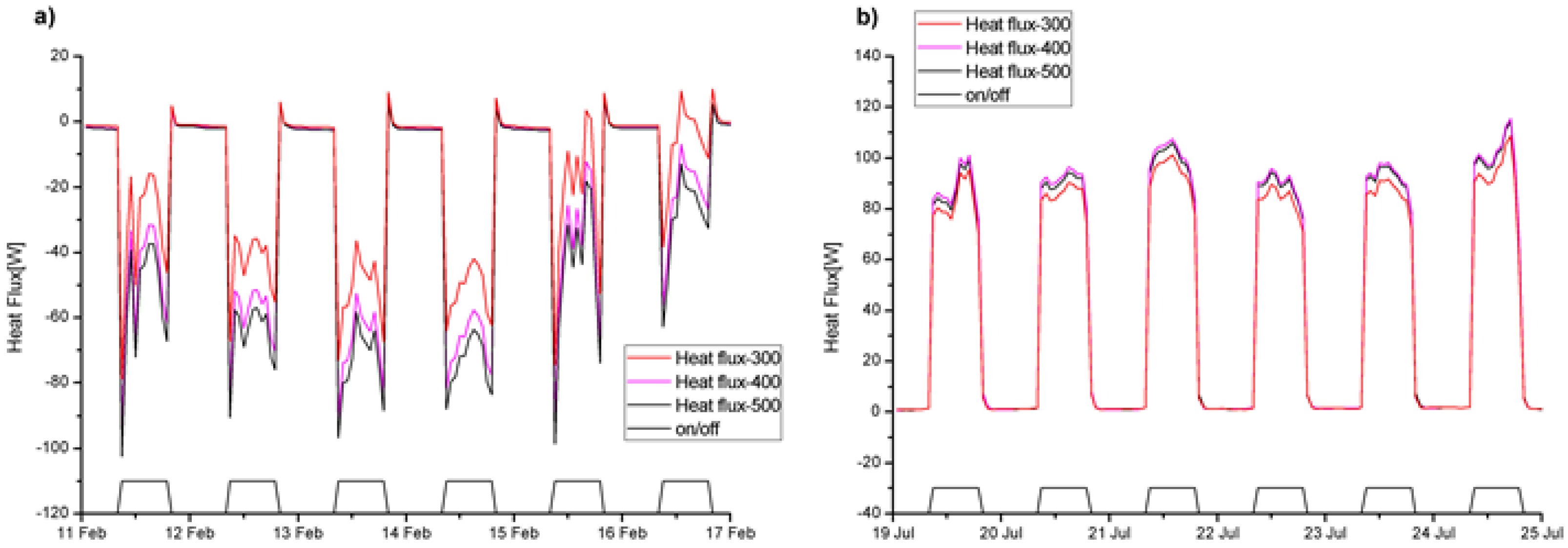
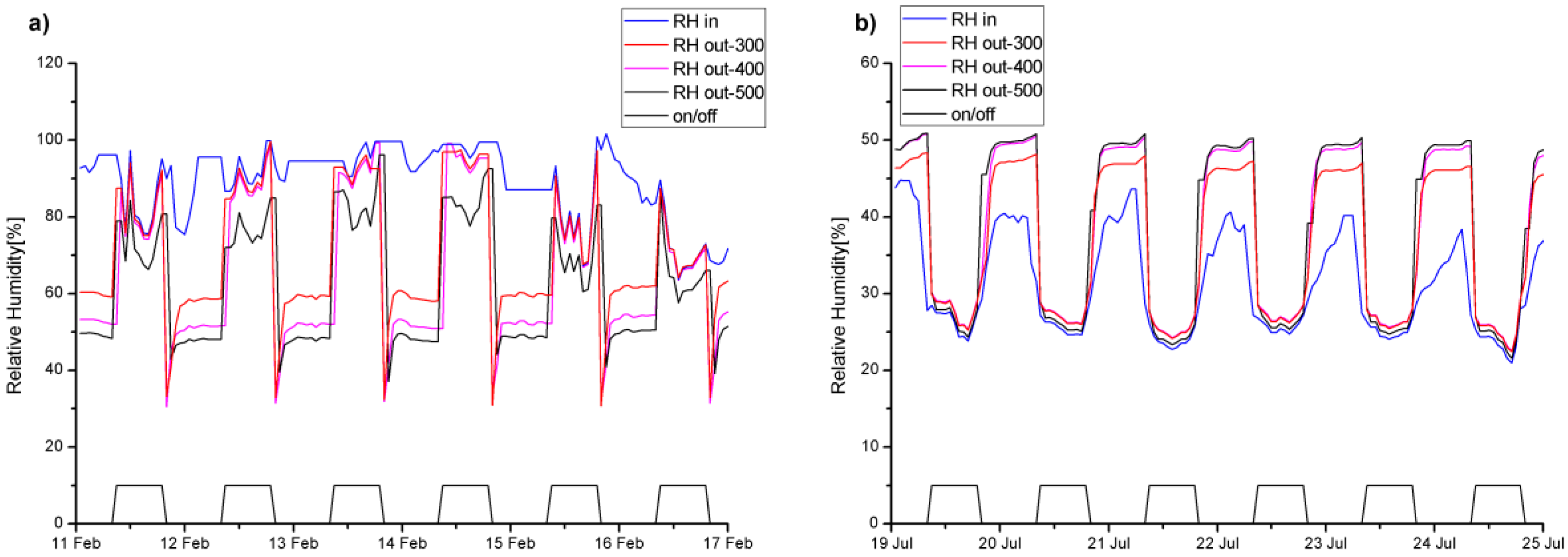
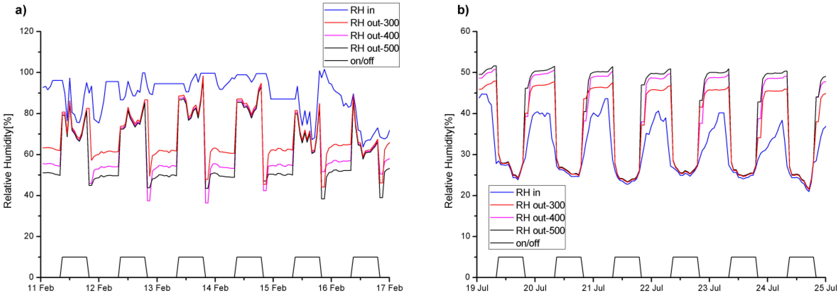
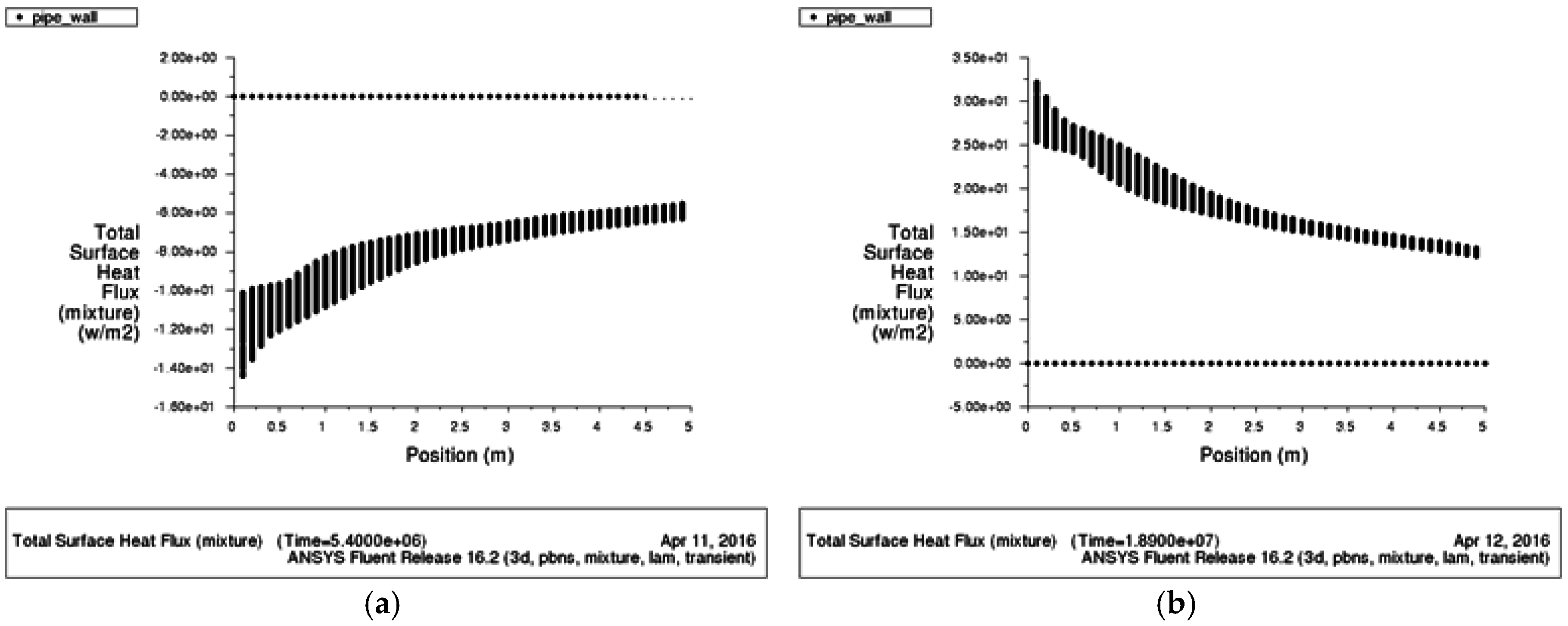
4. Assessments of Heat Flux

As can be seen from the graphs (Figure 20), the heat flow value tends to decrease gradually with pipe length, tending asymptotically to zero. It is evident that the length of the considered pipe (5 m) is not sufficient to reach this limit. It may be appropriate to install a greater length to improve the heat exchanger performance.

The height of the vertical bands also identifies how the pipe is exchanging heat with the ground in correspondence of a given section. The heat exchange tends to diminish gradually for distant sections from the pipe entry point.

As regards the sum of the heat flows that are exchanged in the seasons when the system is switched on and operating, the best performance is obtained (

Table 2. Summation of absolute value heat flux during the plant start-up and on-modes.

Ground Thermal Conductivity W/(mK)	Heat Flux (m3/h)	Winter (kWh)	Summer (kWh)
1	300	23,036	36,631
1	400	25,177	38,681
1	500	25,701	37,412
2	300	24,760	37,544
2	400	25,591	39,840
2	500	26,593	39,720
3	300	25,854	37,327
3	400	25,792	40,077
3	500	26,737	40,724

) in winter and during summer months with a burial depth of 5 m and ground conductivity λ_ground of 3 W/(mK).

5. Conclusions

Energy savings can be achieved in buildings through the adoption of different efficiency improving technological measures. The present work is focused on predicting the performance of an air ground heat exchanger, under different operating conditions.

The air geothermal heat exchanger is a system solution, having no emissions and low energy consumption, used in buildings for mechanical ventilation and cooling. These plants can be appropriate measures to be implemented in nearly zero energy buildings (nZEBs) as a regular exchange of clean air is an important requirement, obtaining treated air through filter selection and, also, an energy intake to air conditioning.

During winter, the simulations have shown that the system cannot pre-treat the air inlet in a satisfactory way during the whole operating period. In fact, during some winter days, the simulations periodically showed a reversal thermal flow between air and ground; for this reason a bypass is necessary.

In summer, the simulations related to the pipe operation revealed significant benefits: the average temperature gain shown is between 2 °C and 3 °C with humidity kept below 60%, obtained with a pipe of 5 m and inlet flow rate of 150 m³/h. In this way it is possible to implement free-cooling avoiding the use of post-treatment with heat pumps.

According to the results, the best performance of the geothermal heat exchanger is obtained at a pipe depth of 5 m with a ground conductivity of λ_ground = 3 W/(mK). These plants are designed for passive houses and nZEBs, where mechanical ventilation is necessary. In future, smart control is expected to improve technical and economic performance. The results about relative humidity below 60% together with the air temperature gain of 2–3 °C in summer time allows to apply free-cooling without using heat pumps in that period, at a burial depth pipe of 5 m with a ground conductivity of λ_ground = 1 W/(mK).

As seen in the results (Table 2), since there is a gain of only 1–2 KWh for each meter of depth, even with the lowest conductivity, an excavation of 3 m is probably sufficient (that is the typical depth of a building excavation) with a ground conductivity of λ_ground = 1 W/(mK). These conditions guarantee about 23 kWh in winter and 37 kWh for free-cooling during summer with a 5 m pipe, demonstrating how the HAGHE system is able to reduce energy consumption in all seasons, and in particular in summer.

References

1. Argiriou, A. Ground cooling. In Passive Cooling of Buildings; Santamouris, M., Asimakopoulos, D., Eds.; Earthscan: New York, NY, USA, 2013; pp. 360–403. [Google Scholar]
2. Ascione, F.; Bellia, L.; Minichiello, F. Earth-to-air heat exchangers for italian climates. Renew. Energy 2011, 36, 2177–2188. [Google Scholar] [CrossRef]
3. Pfafferott, J. Evaluation of earth-to-air heat exchangers with a standardised method to calculate energy efficiency. Energy Build. 2003, 35, 971–983. [Google Scholar] [CrossRef]
4. Lee, K.H.; Strand, R.K. The cooling and heating potential of an earth tube system in buildings. Energy Build. 2008, 40, 486–494. [Google Scholar] [CrossRef]
5. Lee, K.H.; Strand, R.K. Implementation of an earth tube system into energyplus program. In SimBuild 2006, Proceedings of the 2nd National Conference of IBPSA-USA (SimBuild 2006), Cambridge, MA, USA, 2–4 August 2006.
6. Michopoulos, A.; Papakostas, K.T.; Kyriakis, N. Potential of autonomous ground-coupled heat pump system installations in greece. Appl. Energy 2011, 88, 2122–2129. [Google Scholar] [CrossRef]
7. Hackel, S.; Nellis, G.; Klein, S. Optimization of cooling-dominated hybrid ground-coupled heat pump systems. ASHRAE Trans. 2009, 115, 565–580. [Google Scholar]
8. Dickinson, J.; Jackson, T.; Matthews, M.; Cripps, A. The economic and environmental optimisation of integrating ground source energy systems into buildings. Energy 2009, 34, 2215–2222. [Google Scholar] [CrossRef]
9. Bernier, M.A.; Chahla, A.; Pinel, P. Long-term ground-temperature changes in geo-exchange systems. ASHRAE Trans. 2008, 114, 342–350. [Google Scholar]
10. Esen, H.; Inalli, M.; Esen, M. Technoeconomic appraisal of a ground source heat pump system for a heating season in eastern turkey. Energy Convers. Manag. 2006, 47, 1281–1297. [Google Scholar] [CrossRef]
11. Esen, H.; Inalli, M.; Esen, M. A techno-economic comparison of ground-coupled and air-coupled heat pump system for space cooling. Build. Environ. 2007, 42, 1955–1965. [Google Scholar] [CrossRef]
12. Energy Performance Building Directive. 2002. Available online: http://www.bre.co.uk/filelibrary/Scotland/Energy_Performance_of_Buildings_Directive_(EPBD).pdf (accessed on 8 November 2016).
13. Green Paper: Towards a European Strategy for the Security of Energy Supply; European Commission: Brussels, Belgium, 1999.
14. Renewable Energy Target for Europe: 20% by 2020; European Renewable Energy Council: Brussels, Belgium, 2004.
15. Lund, W.J. Present utilization and future prospects of geothermal energy worldwide. In Proceedings of the Renewable Energy 2006 Conference, Chiba, Japan, 9–13 October 2006; pp. 47–52.
16. Andritsos, N.; Arvanitis, A.; Papachristou, M.; Fytikas, M.; Dalambakis, P. Geothermal activities in Greece during 2005–2009. In Proceedings of the World Geothermal Congress, Bali, Indonesia, 25–29 April 2010.
17. Ramamoorthy, M.; Jin, H.; Chiasson, A.D.; Spitler, J.D. Optimal sizing of hybrid ground-source heat pump systems that use a cooling pond as a supplemental heat rejecter—A system simulation approach/discussion. ASHRAE Trans. 2001, 107, 26–38. [Google Scholar]
18. Li, H.; Yang, H. Study on performance of solar assisted air source heat pump systems for hot water production in Hong Kong. Appl. Energy 2010, 87, 2818–2825. [Google Scholar] [CrossRef]
19. Chen, C.; Sun, F.-L.; Feng, L.; Liu, M. Underground water-source loop heat-pump air-conditioning system applied in a residential building in Beijing. Appl. Energy 2005, 82, 331–344. [Google Scholar] [CrossRef]
20. Carlucci, C.; Conciauro, F.; Scremin, B.F.; Antico, A.G.; Muscogiuri, M. Properties of aluminosilicate refractories with synthesized boron-modified TiO2 nanocrystals. Nanomater. Nanotechnol. 2015, 5, 8. [Google Scholar] [CrossRef]
21. Lorusso, C.; Vergaro, V.; Monteduro, A.; Saracino, A.; Ciccarella, G. Characterization of polyurethane foam added with synthesized acetic and oleic-modified TiO2 nanocrystals. Nanomater. Nanotechnol. 2015, 5, 26. [Google Scholar]
22. Conciauro, F.; Filippo, E.; Carlucci, C.; Vergaro, V.; Baldassarre, F. Properties of nanocrystals-formulated aluminosilicate bricks. Nanomater. Nanotechnol. 2015, 5, 28. [Google Scholar] [CrossRef]
23. Tzaferis, A.; Liparakis, D.; Santamouris, M.; Argiriou, A. Analysis of the accuracy and sensitivity of eight models to predict the performance of earth-to-air heat exchangers. Energy Build. 1992, 18, 35–43. [Google Scholar] [CrossRef]
24. Mihalakakou, G.; Santamouris, M.; Asimakopoulos, D. Modelling the thermal performance of earth-to-air heat exchangers. Sol. Energy 1994, 53, 301–305. [Google Scholar] [CrossRef]
25. Bojic, M.; Trifunovic, N.; Papadakis, G.; Kyritsis, S. Numerical simulation, technical and economic evaluation of air-to-earth heat exchanger coupled to a building. Energy 1997, 22, 1151–1158. [Google Scholar] [CrossRef]
26. Gauthier, C.; Lacroix, M.; Bernier, H. Numerical simulation of soil heat exchanger-storage systems for greenhouses. Sol. Energy 1997, 60, 333–346. [Google Scholar] [CrossRef]
27. Hollmuller, P.; Lachal, B. Cooling and preheating with buried pipe systems: Monitoring, simulation and economic aspects. Energy Build. 2001, 33, 509–518. [Google Scholar] [CrossRef]
28. Wu, H.; Wang, S.; Zhu, D. Modelling and evaluation of cooling capacity of earth–air–pipe systems. Energy Convers. Manag. 2007, 48, 1462–1471. [Google Scholar] [CrossRef]
29. Bhutta, M.M.A.; Hayat, N.; Bashir, M.H.; Khan, A.R.; Ahmad, K.N.; Khan, S. CFD applications in various heat exchangers design: A review. Appl. Therm. Eng. 2012, 32, 1–12. [Google Scholar] [CrossRef]
30. Sehli, A.; Hasni, A.; Tamali, M. The potential of earth-air heat exchangers for low energy cooling of buildings in South Algeria. Energy Procedia 2012, 18, 496–506. [Google Scholar] [CrossRef]
31. Cucumo, M.; Cucumo, S.; Montoro, L.; Vulcano, A. A one-dimensional transient analytical model for earth-to-air heat exchangers, taking into account condensation phenomena and thermal perturbation from the upper free surface as well as around the buried pipes. Int. J. Heat Mass Transf. 2008, 51, 506–516. [Google Scholar] [CrossRef]
32. Badescu, V. Simple and accurate model for the ground heat exchanger of a passive house. Renew. Energy 2007, 32, 845–855. [Google Scholar] [CrossRef]
33. Mihalakakou, G.; Santamouris, M.; Asimakopoulos, D.; Tselepidaki, I. Parametric prediction of the buried pipes cooling potential for passive cooling applications. Sol. Energy 1995, 55, 163–173. [Google Scholar] [CrossRef]
34. Kabashnikov, V.P.; Danilevskii, L.N.; Nekrasov, V.P.; Vityaz, I.P. Analytical and numerical investigation of the characteristics of a soil heat exchanger for ventilation systems. Int. J. Heat Mass Transf. 2002, 45, 2407–2418. [Google Scholar] [CrossRef]
35. Tittelein, P.; Achard, G.; Wurtz, E. Corrigendum to “modelling earth-to-air heat exchanger behaviour with the convolutive response factors method” [Appl. Energy 86 (9) 1683–1691]. Appl. Energy 2013, 107, 474. [Google Scholar] [CrossRef]
36. De Paepe, M.; Janssens, A. Thermo-hydraulic design of earth-air heat exchangers. Energy Build. 2003, 35, 389–397. [Google Scholar] [CrossRef]
37. Ozgener, L.; Ozgener, O. An experimental study of the exergetic performance of an underground air tunnel system for greenhouse cooling. Renew. Energy 2010, 35, 2804–2811. [Google Scholar] [CrossRef]
38. Ozgener, O.; Ozgener, L. Determining the optimal design of a closed loop earth to air heat exchanger for greenhouse heating by using exergoeconomics. Energy Build. 2011, 43, 960–965. [Google Scholar] [CrossRef]
39. Al-Ajmi, F.; Loveday, D.L.; Hanby, V.I. The cooling potential of earth–air heat exchangers for domestic buildings in a desert climate. Build. Environ. 2006, 41, 235–244. [Google Scholar] [CrossRef]
40. Woodson, T. Earth-air heat exchangers for passive air conditioning: Case study burkina faso. J. Constr. Dev. Ctries 2012, 17, 21–32. [Google Scholar]
41. Khalajzadeh, V.; Farmahini-Farahani, M.; Heidarinejad, G. A novel integrated system of ground heat exchanger and indirect evaporative cooler. Energy Build. 2012, 49, 604–610. [Google Scholar] [CrossRef]
42. Thiers, S.; Peuportier, B. Thermal and environmental assessment of a passive building equipped with an earth-to-air heat exchanger in France. Sol. Energy 2008, 82, 820–831. [Google Scholar] [CrossRef]
43. Hamada, Y.; Nakamura, M.; Saitoh, H.; Kubota, H.; Ochifuji, K. Improved underground heat exchanger by using no-dig method for space heating and cooling. Renew. Energy 2007, 32, 480–495. [Google Scholar] [CrossRef]
44. Breesch, H.; Bossaer, A.; Janssens, A. Passive cooling in a low-energy office building. Sol. Energy 2005, 79, 682–696. [Google Scholar] [CrossRef]
45. Vaz, J.; Sattler, M.A.; dos Santos, E.D.; Isoldi, L.A. Experimental and numerical analysis of an earth–air heat exchanger. Energy Build. 2011, 43, 2476–2482. [Google Scholar] [CrossRef]
46. Zhao, J.; Wang, H.; Li, X.; Dai, C. Experimental investigation and theoretical model of heat transfer of saturated soil around coaxial ground coupled heat exchanger. Appl. Therm. Eng. 2008, 28, 116–125. [Google Scholar] [CrossRef]
47. Balghouthi, M.; Kooli, S.; Farhat, A.; Daghari, H.; Belghith, A. Experimental investigation of thermal and moisture behaviors of wet and dry soils with buried capillary heating system. Sol. Energy 2005, 79, 669–681. [Google Scholar] [CrossRef]
48. Mihalakakou, G.; Santamouris, M.; Lewis, J.O.; Asimakopoulos, D.N. On the application of the energy balance equation to predict ground temperature profiles. Sol. Energy 1997, 60, 181–190. [Google Scholar] [CrossRef]
49. Li, Z.; Zhu, W.; Bai, T.; Zheng, M. Experimental study of a ground sink direct cooling system in cold areas. Energy Build. 2009, 41, 1233–1237. [Google Scholar] [CrossRef]
50. Rodríguez, R.; Díaz, M.B. Analysis of the utilization of mine galleries as geothermal heat exchangers by means a semi-empirical prediction method. Renew. Energy 2009, 34, 1716–1725. [Google Scholar] [CrossRef]
51. Maerefat, M.; Haghighi, A. Passive cooling of buildings by using integrated earth to air heat exchanger and solar chimney. Renew. Energy 2010, 35, 2316–2324. [Google Scholar] [CrossRef]
52. Eicker, U.; Vorschulze, C. Potential of geothermal heat exchangers for office building climatisation. Renew. Energy 2009, 34, 1126–1133. [Google Scholar] [CrossRef]
53. Ghosal, M.; Tiwari, G.; Das, D.; Pandey, K. Modeling and comparative thermal performance of ground air collector and earth air heat exchanger for heating of greenhouse. Energy Build. 2005, 37, 613–621. [Google Scholar] [CrossRef]
54. Bisoniya, T.S.; Kumar, A.; Baredar, P. Experimental and analytical studies of earth–air heat exchanger (eahe) systems in India: A review. Renew. Sustain. Energy Rev. 2013, 19, 238–246. [Google Scholar] [CrossRef]
55. Bansal, V.; Misra, R.; Agarwal, G.D.; Mathur, J. “Derating factor” new concept for evaluating thermal performance of earth air tunnel heat exchanger: A transient CFD analysis. Appl. Energy 2013, 102, 418–426. [Google Scholar] [CrossRef]
56. Ozgener, L. A review on the experimental and analytical analysis of earth to air heat exchanger (EAHE) systems in Turkey. Renew. Sustain. Energy Rev. 2011, 15, 4483–4490. [Google Scholar] [CrossRef]
57. Misra, R.; Bansal, V.; Agrawal, G.D.; Mathur, J.; Aseri, T. Transient analysis based determination of derating factor for earth air tunnel heat exchanger in summer. Energy Build. 2013, 58, 103–110. [Google Scholar] [CrossRef]
58. Congedo, P.M.; Colangelo, G.; Starace, G. CFD simulations of horizontal ground heat exchangers: A comparison among different configurations. Appl. Therm. Eng. 2012, 33–34, 24–32. [Google Scholar] [CrossRef]
59. Congedo, P.; Lorusso, C.; De Giorgi, M.; Laforgia, D. Computational fluid dynamic modeling of horizontal air-ground heat exchangers (HAGHE) for HVAC systems. Energies 2014, 7, 8465. [Google Scholar] [CrossRef]
60. ANSYS Inc. ANSYS FLUENT Release 14.0 User Manual; ANSYS Inc.: Canonsburg, PA, USA, 2011. [Google Scholar]
61. Lee, E. Development, Verification and Implementation of a Horizontal Buried Pipe Ground Heat Transfer Model in Energy Plus; ProQuest: Ann Arbor, MI, USA, 2008; p. 211. [Google Scholar]
62. Niu, F.; Yu, Y.; Yu, D.; Li, H. Heat and mass transfer performance analysis and cooling capacity prediction of earth to air heat exchanger. Appl. Energy 2015, 137, 211–221. [Google Scholar] [CrossRef]
63. Thermo Technical Committee Italian Energy and Environment. UNI EN ISO 15927-4. 2012. Available online: http://shop.cti2000.it (accessed on 8 November 2016).
Figure 1. (a) Operating principle of the air-heat exchanger in winter; and (b) operating principle of the air-heat exchanger in summer.
Energies 09 00930 g001
Figure 2. Temperature vs. Time (h)—Performance of horizontal air-ground heat exchanger (HAGHE) for different ground conductivity values—Depth = 3 m: (a) winter period; and (b) summer period.
Energies 09 00930 g002
Figure 3. Temperature vs. Time (h)—Performance of HAGHE for different ground conductivity values—Depth = 4 m: (a) winter period; and (b) summer period.
Energies 09 00930 g003
Figure 4. Temperature vs. Time (h)—Performance of HAGHE for different ground conductivity values—Depth = 5 m: (a) winter period; and (b) summer period.
Energies 09 00930 g004
Figure 5. Heat flux vs. Time (h)—Performance of HAGHE for different ground conductivity values—Depth = 3 m: (a) winter period; and (b) summer period.
Energies 09 00930 g005
Figure 6. Heat flux vs. Time (h)—Performance of HAGHE for different ground conductivity values—Depth = 4 m: (a) winter period; and (b) summer period.
Energies 09 00930 g006
Figure 7. Heat flux vs. Time (h)—Performance of HAGHE for different ground conductivity values—Depth = 5 m: (a) winter period; and (b) summer period.
Energies 09 00930 g007
Figure 8. Relative humidity vs. Time (h)—Performance of HAGHE for different ground conductivity values—Depth = 3 m: (a) winter period; and (b) summer period.
Energies 09 00930 g008
Figure 9. Relative humidity vs. Time (h)—Performance of HAGHE for different ground conductivity values—Depth = 4 m: (a) winter period; and (b) summer period.
Energies 09 00930 g009
Figure 10. Relative humidity vs. Time (h)—Performance of HAGHE for different ground conductivity values—Depth = 5 m: (a) winter period; and (b) summer period.
Energies 09 00930 g010
Figure 11. Temperature vs. Time (h)—Performance of HAGHE for different pipe burial depths—λground = 1 W/(mK): (a) winter period; and (b) summer period.
Energies 09 00930 g011
Figure 12. Temperature vs. Time (h)—Performance of HAGHE for different pipe burial depths—λground = 2 W/(mK): (a) winter period; and (b) summer period.
Energies 09 00930 g012
Figure 13. Temperature vs. Time (h)—Performance of HAGHE for different pipe burial depths—λground = 3 W/(mK): (a) winter period; and (b) summer period.
Energies 09 00930 g013
Figure 14. Heat flux vs. Time (h)—Performance of HAGHE for different pipe burial depths—λground = 1 W/(mK): (a) winter period; and (b) summer period.
Energies 09 00930 g014
Figure 15. Heat flux vs. Time (h)—Performance of HAGHE for different pipe burial depths—λground = 2 W/(mK): (a) winter period; and (b) summer period.
Energies 09 00930 g015
Figure 16. Heat flux vs. Time (h)—Performance of HAGHE for different pipe burial depths—λground = 3 W/(mK): (a) winter period; and (b) summer period.
Energies 09 00930 g016
Figure 17. Relative humidity vs. Time (h)—Performance of HAGHE for different pipe burial depths—λground = 1 W/(mK): (a) winter period; and (b) summer period.
Energies 09 00930 g017
Figure 18. Relative humidity vs. Time (h)—Performance of HAGHE for different pipe burial depths—λground = 2 W/(mK): (a) winter period; and (b) summer period.
Energies 09 00930 g018
Figure 19. Relative humidity vs. Time (h)—Performance of HAGHE for different pipe burial depths—λground = 3 W/(mK): (a) winter period; and (b) summer period.
Energies 09 00930 g019
Figure 20. (a) Total surface heat flux in winter; and (b) total surface heat flux in summer.
Energies 09 00930 g020