
The Coupling Fields Characteristics of Cable Joints and Application in the Evaluation of Crimping Process Defects


Abstract
:1. Introduction
2. The Coupling Field Analysis Model of Cable Joints under Crimping Process Defects
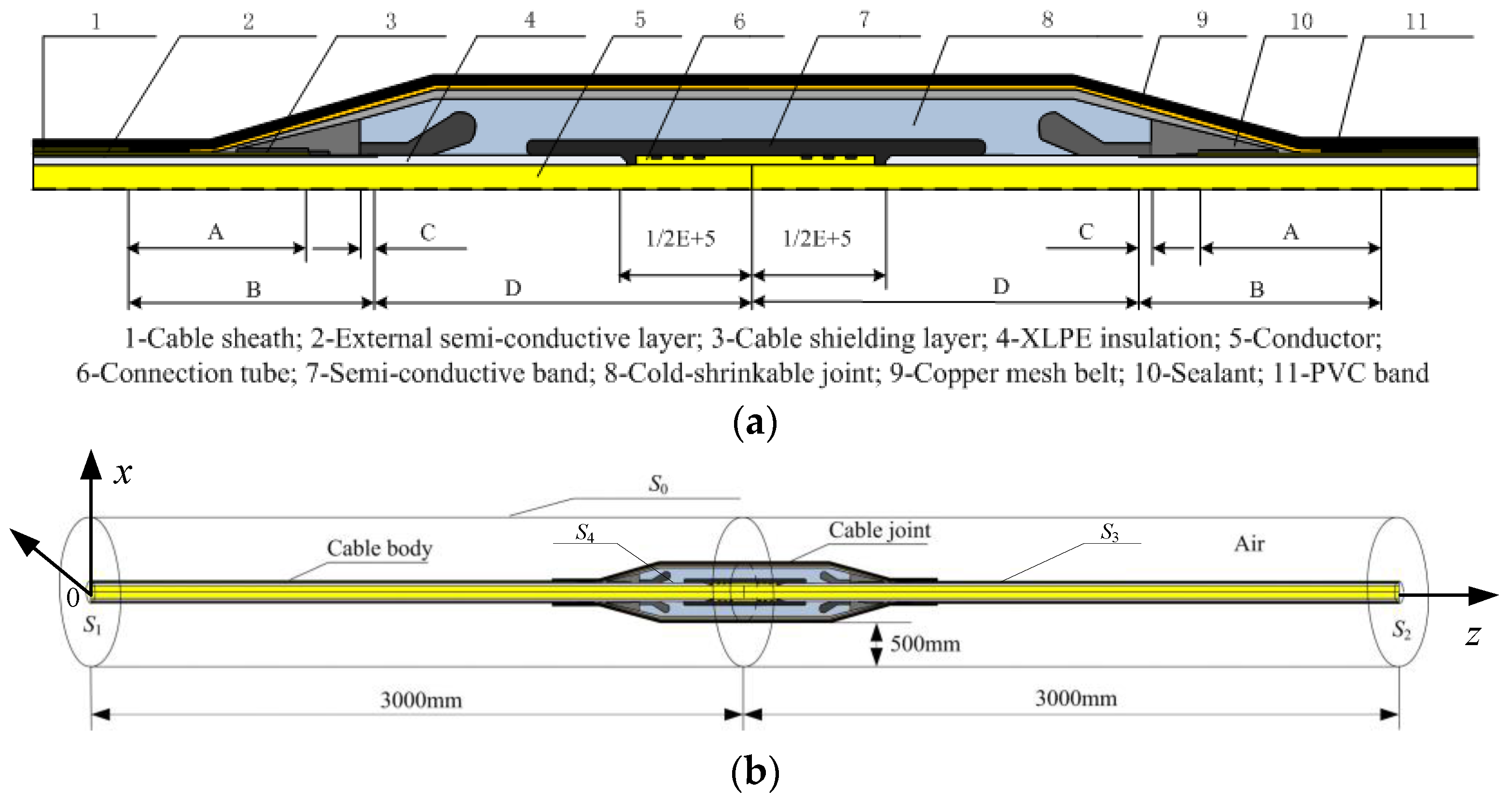
2.1. The Physics Fields Computation of Cable Joints
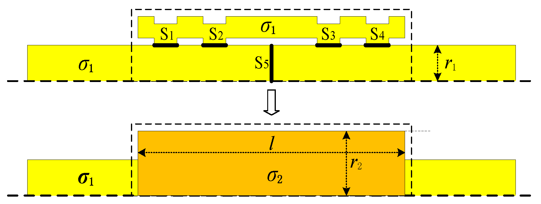
2.2. The Equivalent Model of Cable Joint under Crimping Process Defects
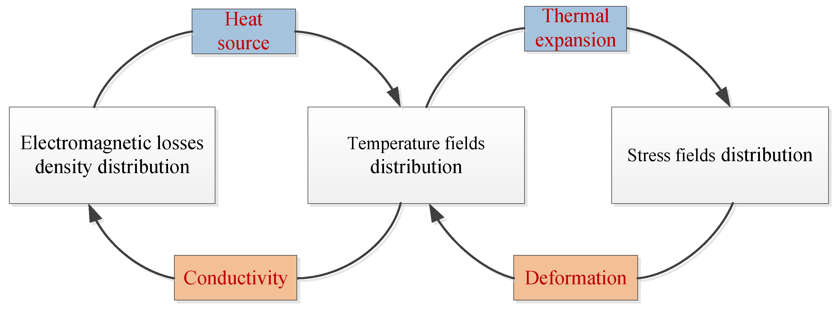
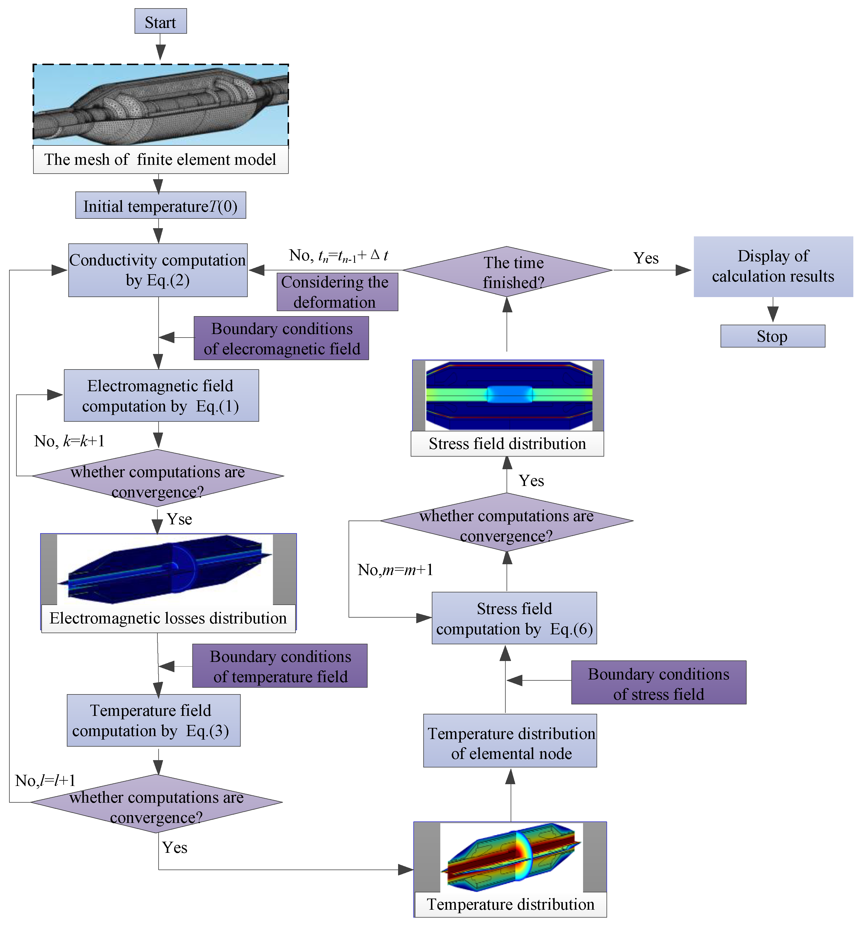
2.3. The Coupling Field Computation of Cable Joints under Crimping Process Defects
2.4. Example Calculation
3. Analysis of Thermal-Mechanical Characteristics under Crimping Process Defects
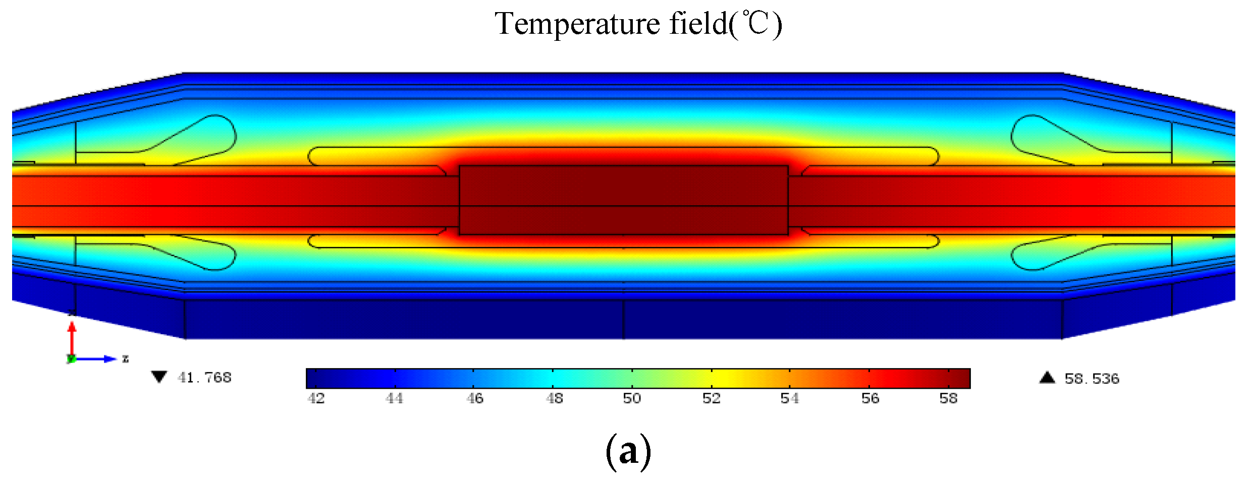
3.1. Analysis of Thermal Characteristics
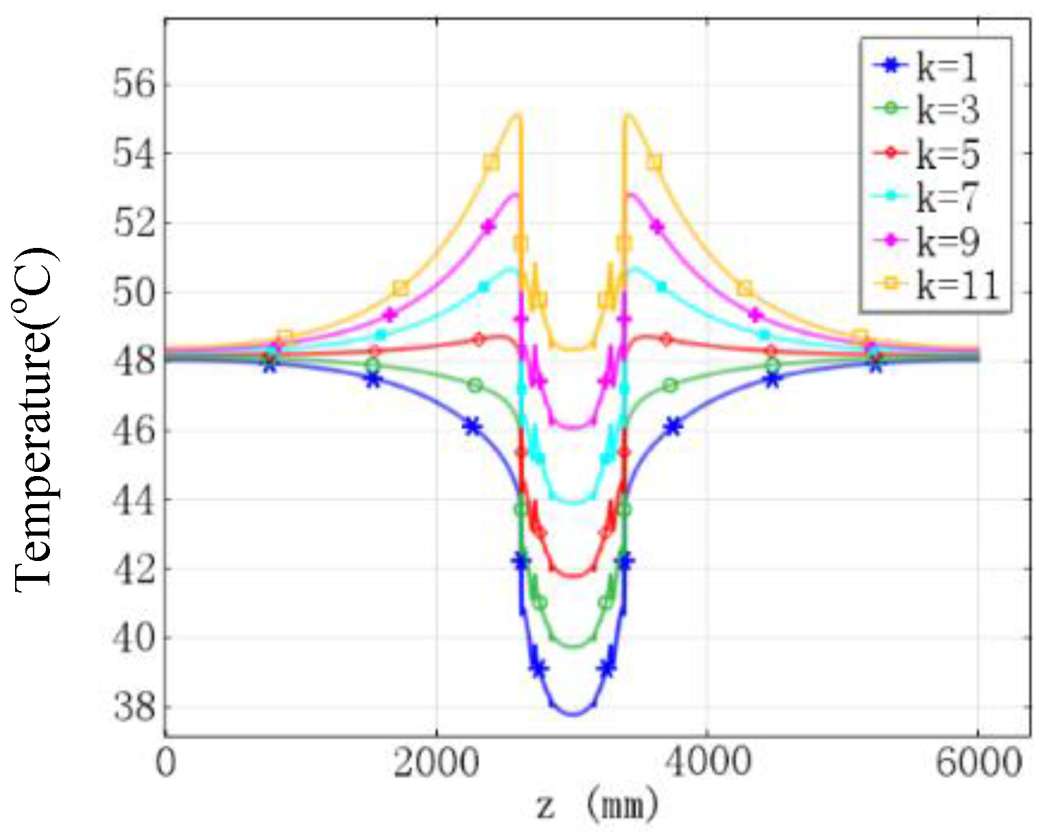
3.1.1. The Influence of Contact Coefficient k
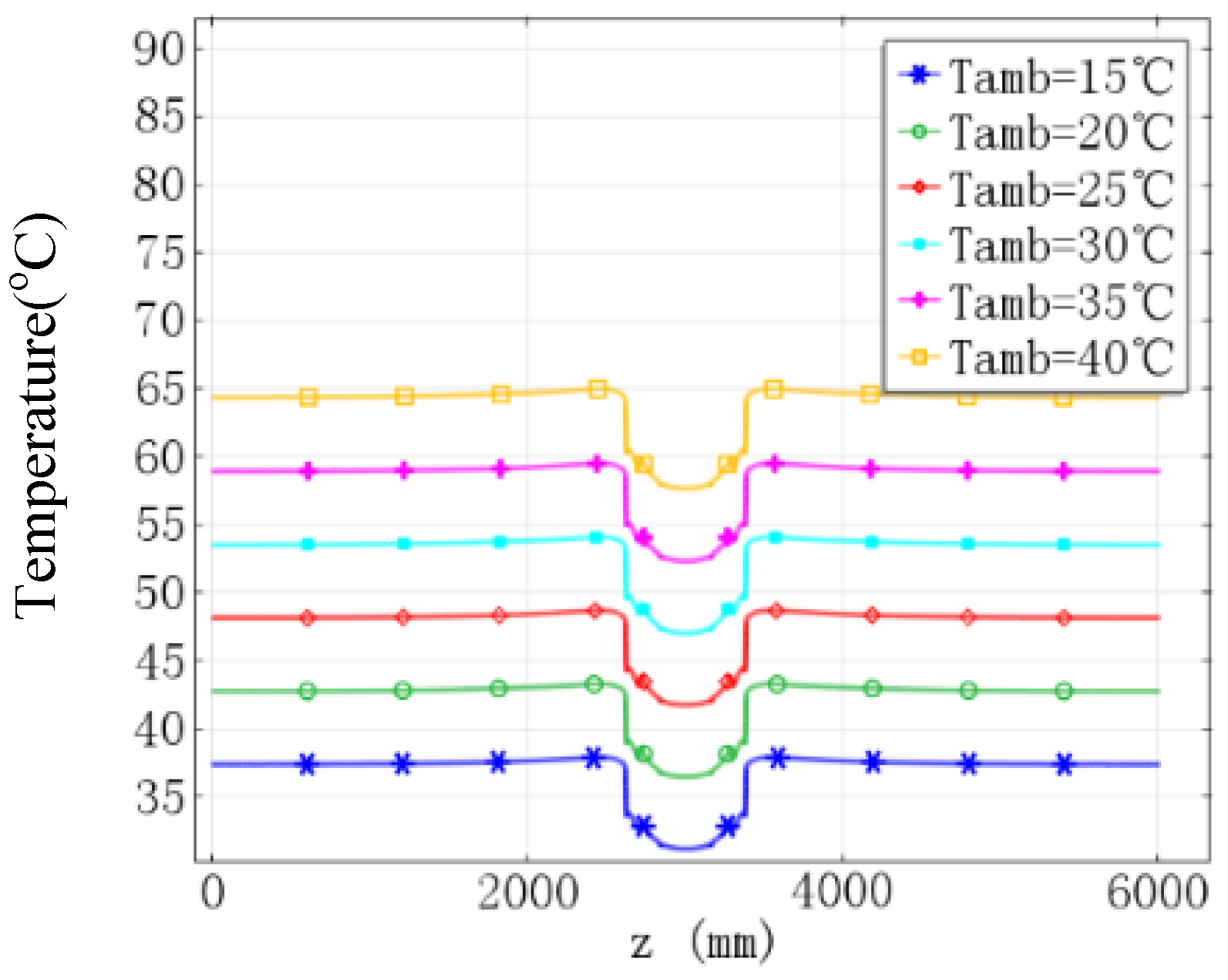
3.1.2. The Influence of Ambient Temperature Tamb
3.1.3. The Influence of Load Current I
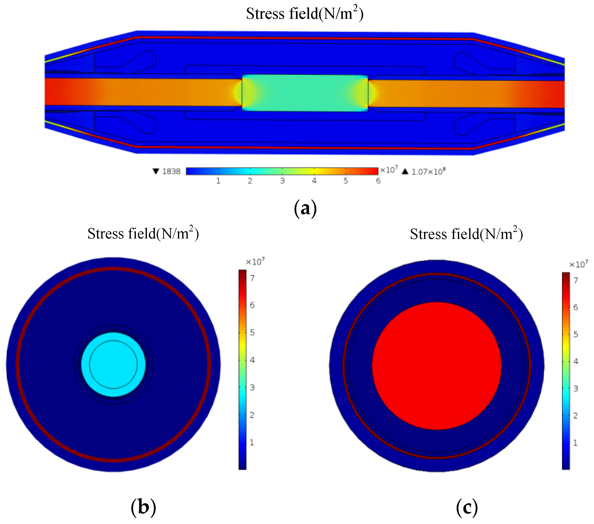
3.2. Analysis of Stress Characteristics
3.2.1. The Influence of Contact Coefficient k
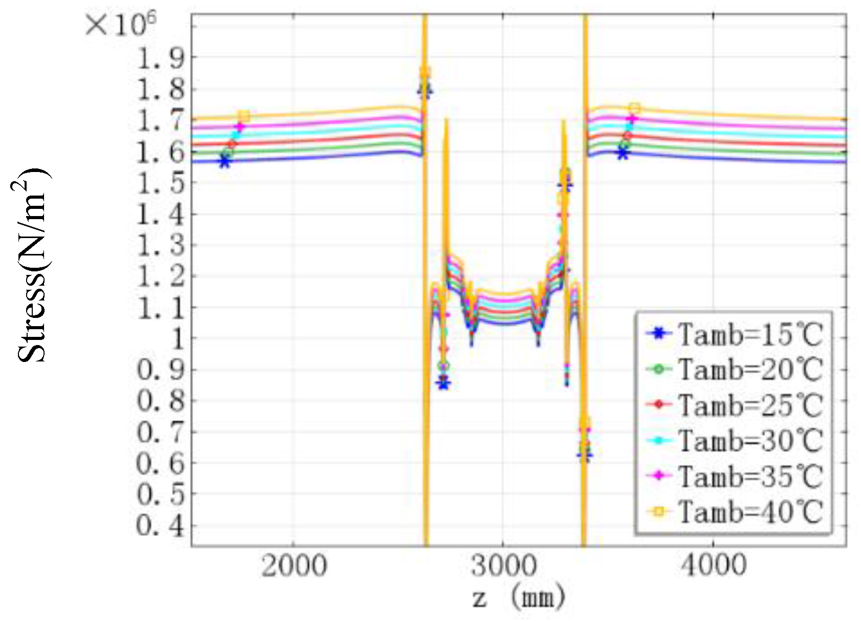
3.2.2. The Influence of Ambient Temperature Tamb
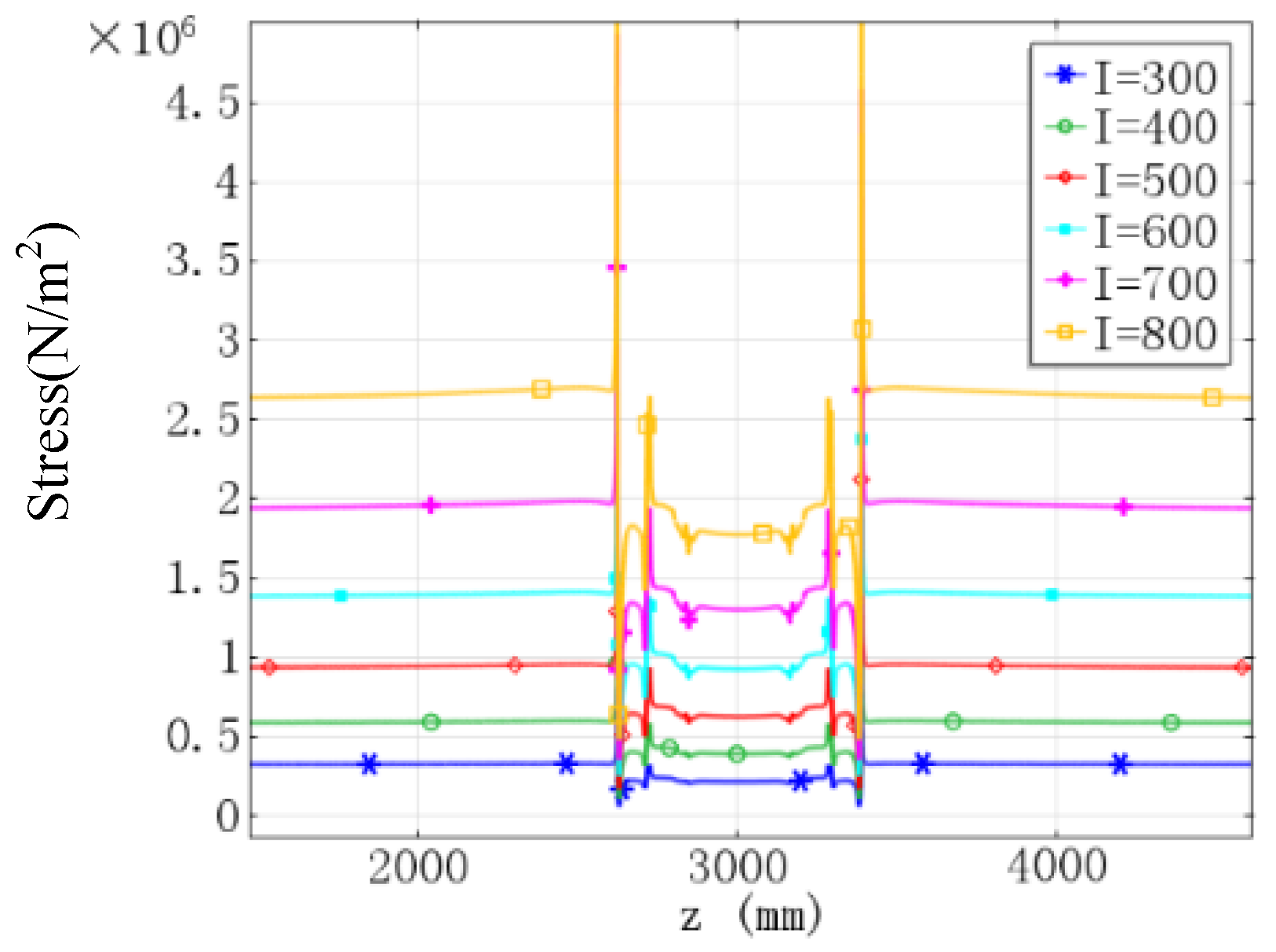
3.2.3. The Influence of Load Current I
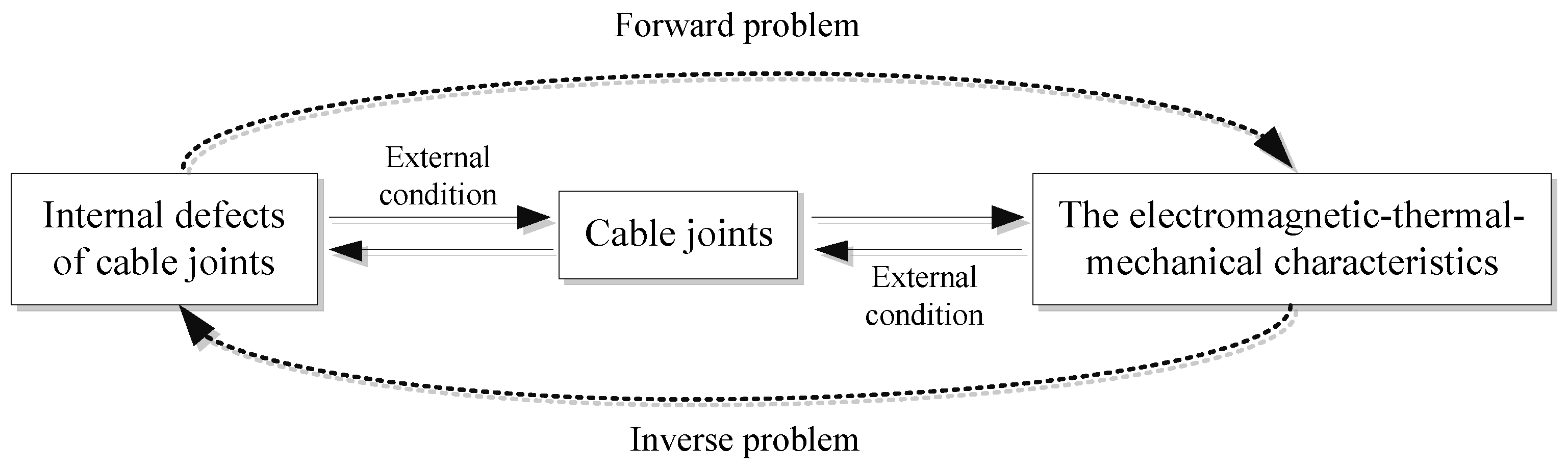
4. Evaluation of Internal Defect States of Cable Joint under Crimping Process Defects
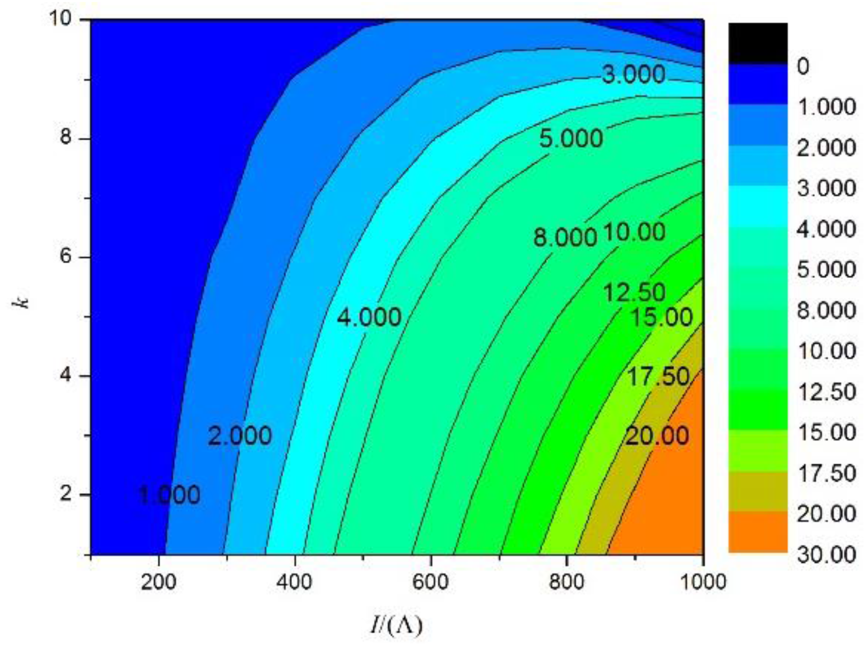
4.1. Evaluation Results and Analysis Based on Temperature Characteristic
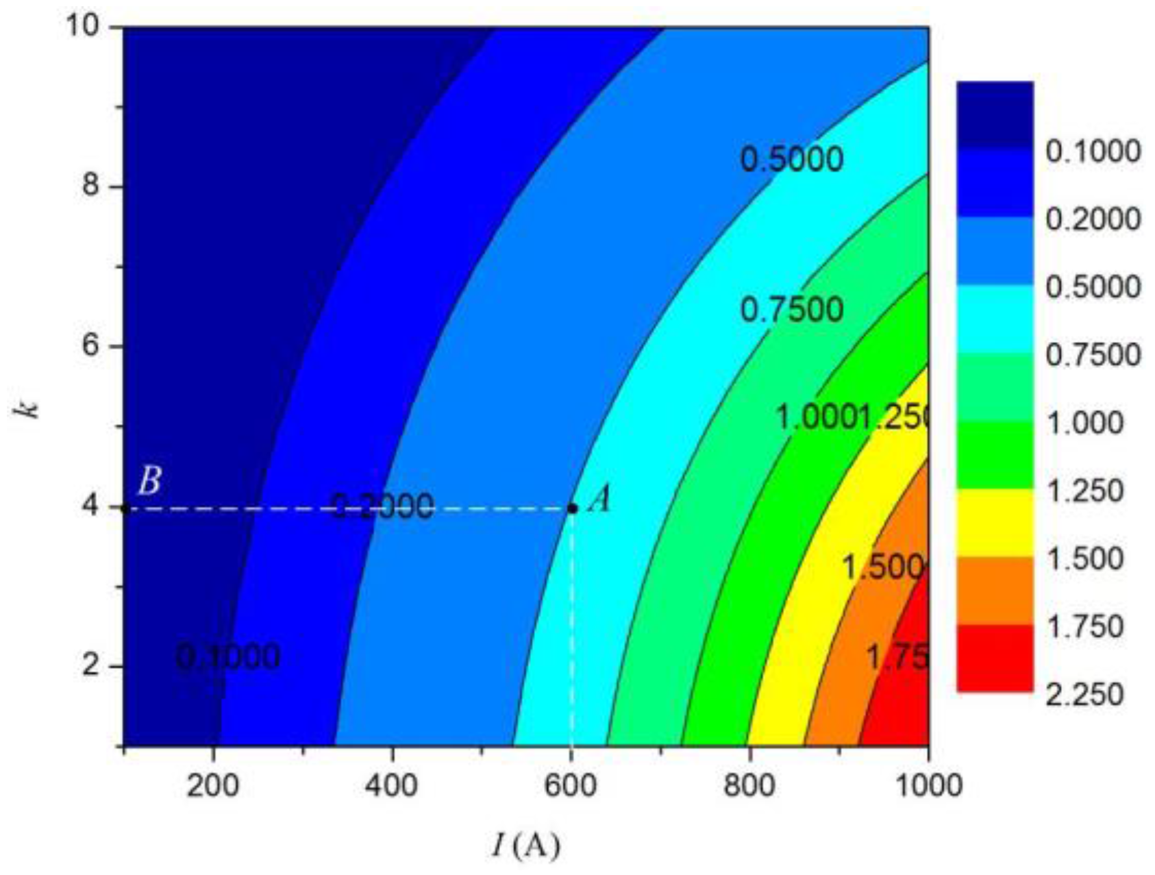
4.2. Evaluation Results and Analysis Based on Stress Characteristic
5. Experimental Verification
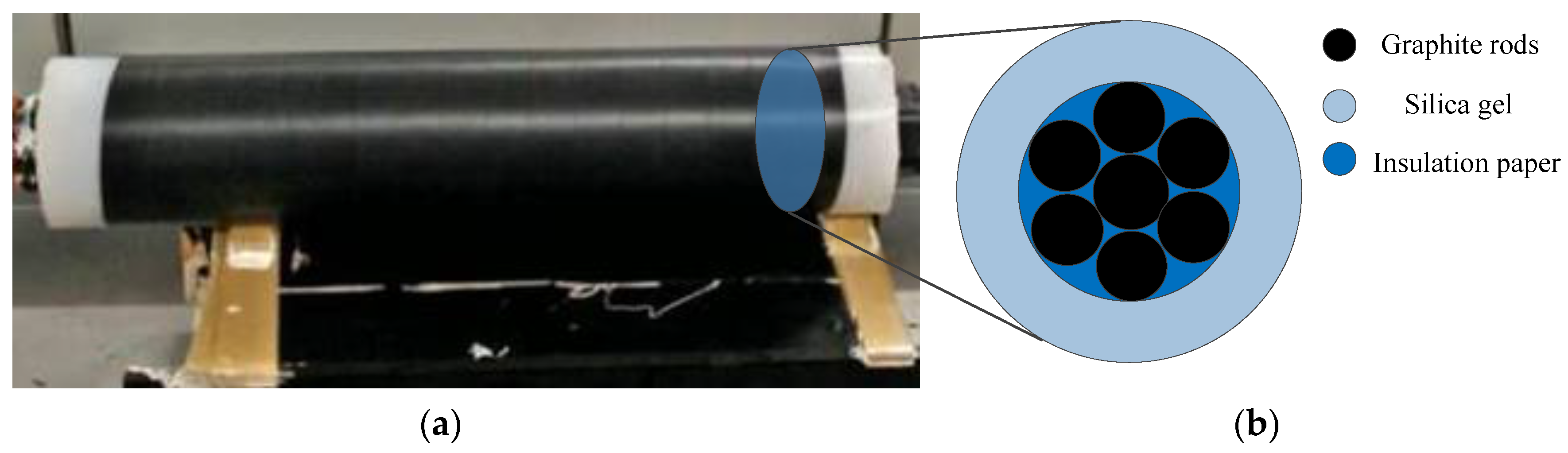
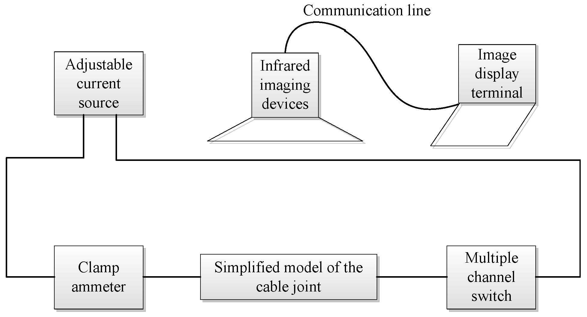
5.1. Experiment Setup
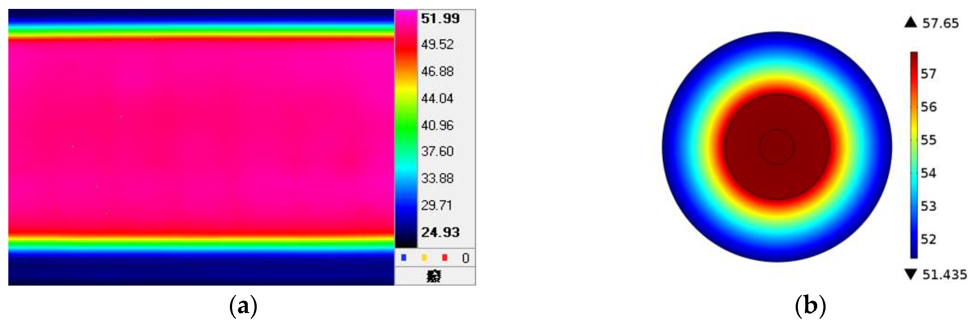
5.2. Results and Discussion
6. Conclusions
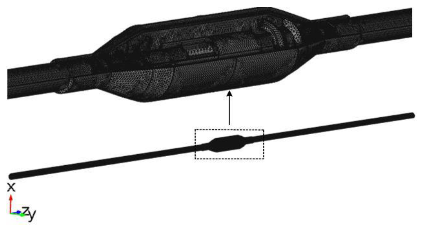
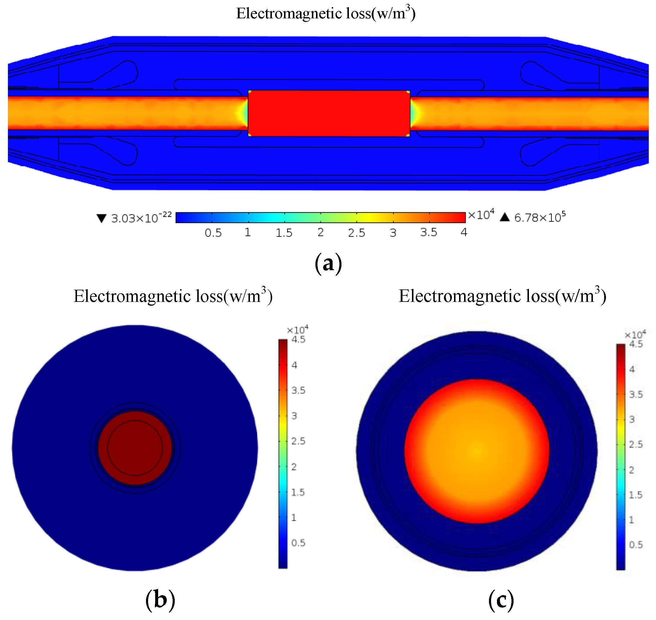
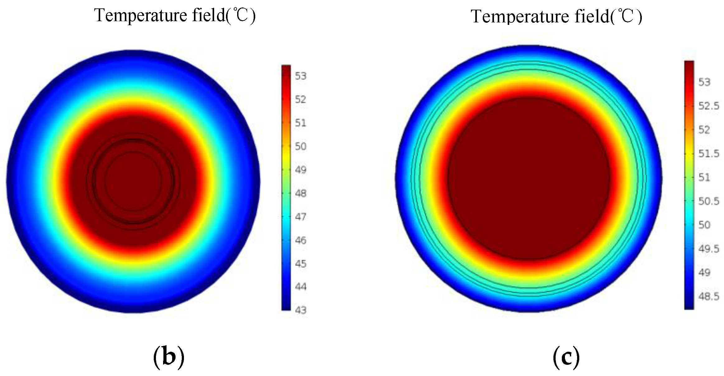
- This paper establishes an electromagnetic-thermal-mechanical coupling analysis model based on the finite element method. The crimping process defects of cable joints are characterized by their contact resistances by solving the equivalent conductivity of the cable joint. Based on this model, the electromagnetic losses distribution, temperature distribution and stress distribution of a cable have been calculated.
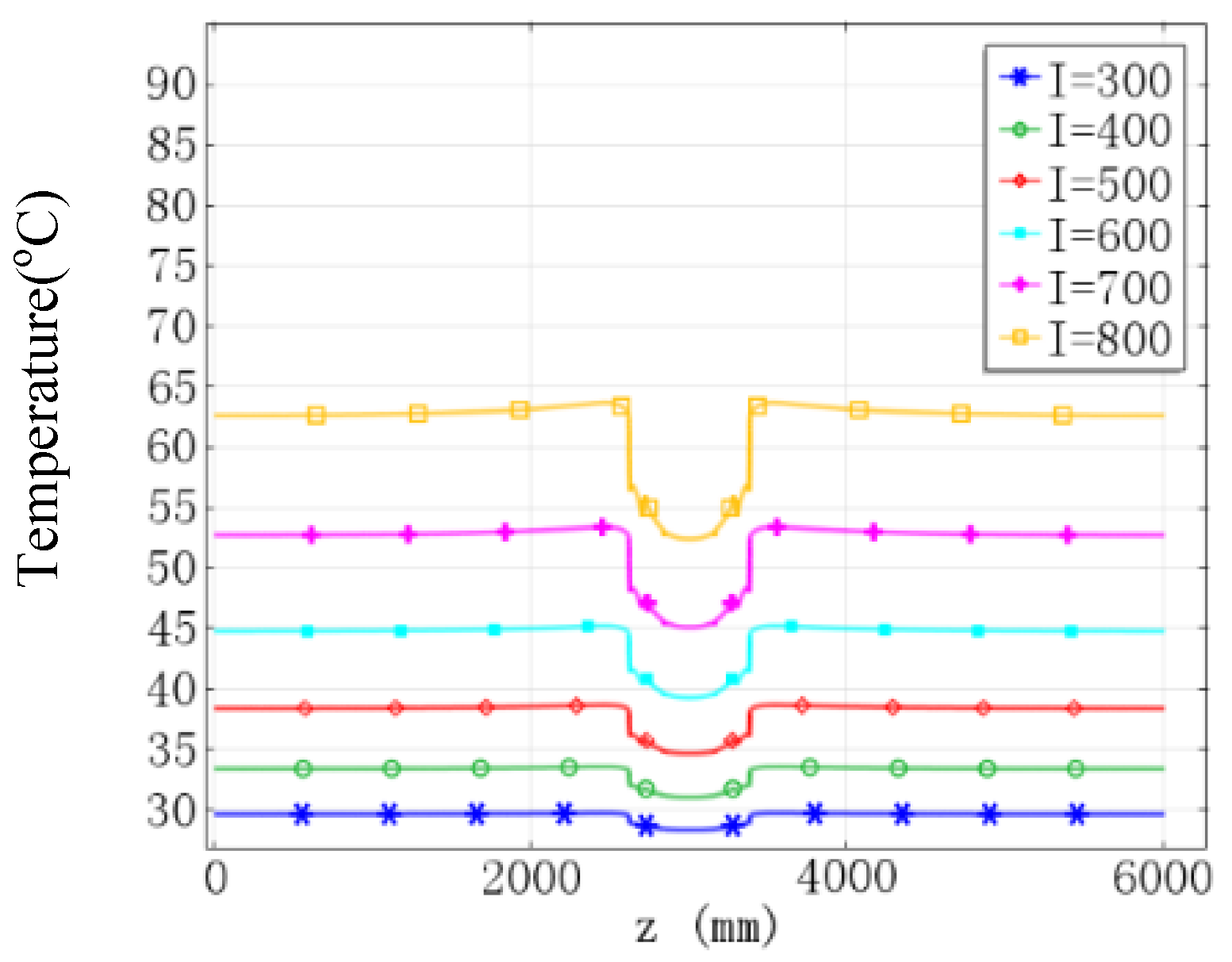
- Based on this model, the coupling fields characteristics for different contact coefficients k, ambient temperatures Tamb and load currents I were analyzed, which indicates that the internal defects of cable joints can be evaluated.
- According to the thermal-stress characteristics of cable joints under internal defects, this paper uses the temperature difference ΔTf and stress difference Δσf of the cable surface to evaluate the internal defects of cable joints and proposes an evaluation method for internal defects of cable joints.
- Simplified cable joint experiments which can simulate the temperature distribution of the cable and perform different defects tests are done and they verify the accuracy of the coupling field analysis model proposed in this paper.
Acknowledgments
Author Contributions
Conflicts of Interest
Nomenclature
| μ | permeability |
| A | magnetic vector potential |
| σ | conductivity of cable joint |
| Js | applied current density |
| ω | angular frequency |
| σ20 | conductivity at 20 °C |
| α | temperature coefficient |
| T | temperature |
| λ | thermal conductivity |
| Qv | heat source per unit volume |
| h | coefficient of convective heat transfer |
| hr | coefficient of radiation heat transfer |
| Tf | surface temperature |
| Ta | temperature of air |
| Tamb | ambient temperature |
| n | normal vector |
| σ0 | Stefan-Boltzmann constant |
| ε | surface emissivity |
| σ1 | conductivity of cable conductor |
| σ2 | equivalent conductivity |
| k | contact coefficient |
| I | load current |
| θ | stress tensor |
| f | externally applied force |
| ρ | material density |
| u | displacement |
| t | time |
| γ | damping coefficient |
| η | strain tensor |
| ηE | elastic strain component |
| ηTh | thermal strain component |
| D | strain coefficient |
| α | linear expansion coefficient |
| E(T) | young’s modulus |
| υ | Poisson’s ratio of material |
| ΔTf | surface temperature difference |
| Δσf | stress difference |
| Tbf | surface temperatures of cable body |
| Tjf | surface temperatures of cable joint |
References
- Cho, J.; Kim, J.-H.; Lee, H.-J.; Kim, J.-Y.; Song, I.-K.; Choi, J.-H. Development and Improvement of an Intelligent Cable Monitoring System for Underground Distribution Networks Using Distributed Temperature Sensing. Energies 2014, 7, 1076–1094. [Google Scholar] [CrossRef]
- Benato, R.; Dambone Sessa, S.; Guglielmi, F.; Partal, E.; Tleis, N. Ground Return Current Behaviour in High Voltage Alternating Current Insulated Cables. Energies 2014, 7, 8116–8131. [Google Scholar] [CrossRef]
- Benato, R.; Napolitano, D. Overall Cost Comparison Between Cable and Overhead Lines Including the Costs for Repair After Random Failures. IEEE Trans. Power Deliv. 2012, 27, 1213–1222. [Google Scholar] [CrossRef]
- Benato, R.; Napolitano, D. State-space model for availability assessment of EHV OHL–UGC mixed power transmission link. Electr. Power Syst. Res. 2013, 99, 45–52. [Google Scholar] [CrossRef]
- Stancu, C.; Notingher, P.; Ciuprina, F.; Notingher, P., Jr.; Castellon, J.; Agnel, S.; Toureille, A. Computation of the Electric Field in Cable Insulation in the Presence of Water Trees and Space Charge. IEEE Trans. Ind. Appl. 2009, 45, 30–43. [Google Scholar] [CrossRef]
- Kroener, E.; Vallati, A.; Bittelli, M. Numerical simulation of coupled heat, liquid water and water vapor in soils for heat dissipation of underground electrical power cables. Appl. Therm. Eng. 2014, 70, 510–523. [Google Scholar] [CrossRef]
- Olsen, R.; Anders, G.J.; Holboell, J.; Gudmundsdóttir, U.S. Modelling of Dynamic Transmission Cable Temperature Considering Soil-Specific Heat, Thermal Resistivity, and Precipitation. IEEE Trans. Power Deliv. 2013, 28, 1909–1917. [Google Scholar] [CrossRef]
- Aras, F.; Alekperov, V.; Can, N.; Kirkici, H. Aging of 154 kV underground power cable insulation under combined thermal and electrical stresses. IEEE Electr. Insul. Mag. 2007, 23, 25–33. [Google Scholar] [CrossRef]
- Mecheri, Y.; Boukezzi, L.; Boubakeur, A.; Lallouani, M. Dielectric and mechanical behavior of cross-linked polyethylene under thermal aging. In Proceedings of the Annual Report Conference on Electrical Insulation and Dielectric Phenomena, Victoria, CA, USA, 15–18 October 2000; pp. 560–563.
- Tzimas, A.; Rowland, S.; Dissado, L.A.; Fu, M.; Nilsson, U.H. Effect of long-time electrical and thermal stresses upon the endurance capability of cable insulation material. IEEE Trans. Dielectr. Electr. Insul. 2009, 16, 1436–1443. [Google Scholar] [CrossRef]
- Shaker, Y.O.; El-Hag, A.H.; Patel, U.; Jayaram, S.H. Thermal modeling of medium voltage cable terminations under square pulses. IEEE Trans. Dielectr. Electr. Insul. 2014, 21, 932–939. [Google Scholar] [CrossRef]
- Gu, J.; Li, X.; Yin, Y. Calculation of electric field and temperature field distribution in MVDC polymeric power cable. In Proceedings of the IEEE International Conference Properties and Applications of Dielectric Materials, Harbin, China, 19–23 July 2009; pp. 105–108.
- Choo, W.; Chen, G.; Swingler, S.G. Electric field in polymeric cable due to space charge accumulation under DC and temperature gradient. IEEE Trans. Dielectr. Electr. Insul. 2011, 18, 596–606. [Google Scholar] [CrossRef]
- Illias, H.A.; Lee, Z.H.; Bakar, A.H.A.; Mokhlis, H.; Mohd Ariffin, A. Distribution of electric field in medium voltage cable joint geometry. In Proceedings of the International Conference on Condition Monitoring and Diagnosis (CMD), Bali, Indonesia, 23–27 September 2012; pp. 1051–1054.
- Illias, H.A.; Ng, Q.L.; Bakar, A.H.A.; Mokhlis, H.; Ariffin, A.M. Electric field distribution in 132 kV XLPE cable termination model from finite element method. In Proceedings of the International Conference on Condition Monitoring and Diagnosis (CMD), Bali, Indonesia, 23–27 September 2012; pp. 80–83.
- Lachini, S.; Gholami, A.; Mirzaie, M. The simulation of electric field distribution on cable under the presence of moisture and air voids. In Proceedings of the 4th International Power Engineering and Optimization Conference (PEOCO), Shah Alam, Malaysia, 23–24 June 2010; pp. 149–153.
- Ying, Q.; Wei, D.; Gao, X.; Chen, P. Development of high voltage XLPE power cable system in China. In Proceedings of the 6th International Conference on Properties and Applications of Dielectric Materials, Xi’an, China, 21–26 June 2000; pp. 247–253.
- Luo, J.; Shi, J.; Yuan, J. Study on Surface Discharge of Composite Dielectric in XLPE Power Cable Joints. High Volt. Eng. 2001, 4, 341–343. [Google Scholar]
- Yoshida, S.; Tan, M.; Yagi, S.; Seo, S.; Isaka, M. Development of prefabricated type joint for 275 kV XLPE cable. In Proceedings of the IEEE International Symposium on Electrical Insulation Conference, Toronto, ON, Canada, 3–6 June 1990; pp. 290–295.
- Anders, G.J.; Chaaban, M.; Bedard, N.; Ganton, R.W.D. New Approach to Ampacity Evaluation of Cables in Ducts Using Finite Element Technique. IEEE Trans. Power Deliv. 1987, 285, 969–975. [Google Scholar] [CrossRef]
- Chatziathanasiou, V.; Chatzipanagiotou, P.; Papagiannopoulos, I.; De Mey, G.; Więcek, B. Dynamic thermal analysis of underground medium power cables using thermal impedance, time constant distribution and structure function. Appl. Therm. Eng. 2013, 60, 256–260. [Google Scholar] [CrossRef]
- Sedaghat, A.; De Leon, F. Thermal Analysis of Power Cables in Free Air: Evaluation and Improvement of the IEC Standard Ampacity Calculations. IEEE Trans. Power Deliv. 2014, 29, 2306–2314. [Google Scholar] [CrossRef]
- Canova, A.; Freschi, F.; Giaccone, L.; Guerrisi, A. The high magnetic coupling passive loop: A steady-state and transient analysis of the thermal behavior. Appl. Therm. Eng. 2012, 37, 154–164. [Google Scholar] [CrossRef]
- Anders, G.J.; Coates, M.; Chaaban, M. Ampacity Calculations for Cables in Shallow Troughs. IEEE Trans. Power Deliv. 2010, 25, 2064–2072. [Google Scholar] [CrossRef]
- Pilgrim, J.A.; Lewin, P.L.; Larsen, S.T.; Waite, F.; Payne, D. Rating of Cables in Unfilled Surface Troughs. IEEE Trans. Power Deliv. 2012, 27, 993–1001. [Google Scholar] [CrossRef]
- Yang, F.; Cheng, P.; Luo, H.; Yang, Y.; Liu, H.; Kang, K. 3-D thermal analysis and contact resistance evaluation of power cable joint. Appl. Therm. Eng. 2016, 93, 1183–1192. [Google Scholar] [CrossRef]


| Equation | |
| Parameters | A = 0.06123 B = 66.23295 C = 1051.6936 D = 414.48237 E = 5.62593 F = −3.13981 |
| Correlation coefficient | 0.99115 |
| Equation | |
| Parameters | A = 0.0052 B = 5.16572 C = 1041.9008 D = 411.43753 E = 6.06807 F = −4.33966 |
| Correlation Coefficient | 0.9965 |
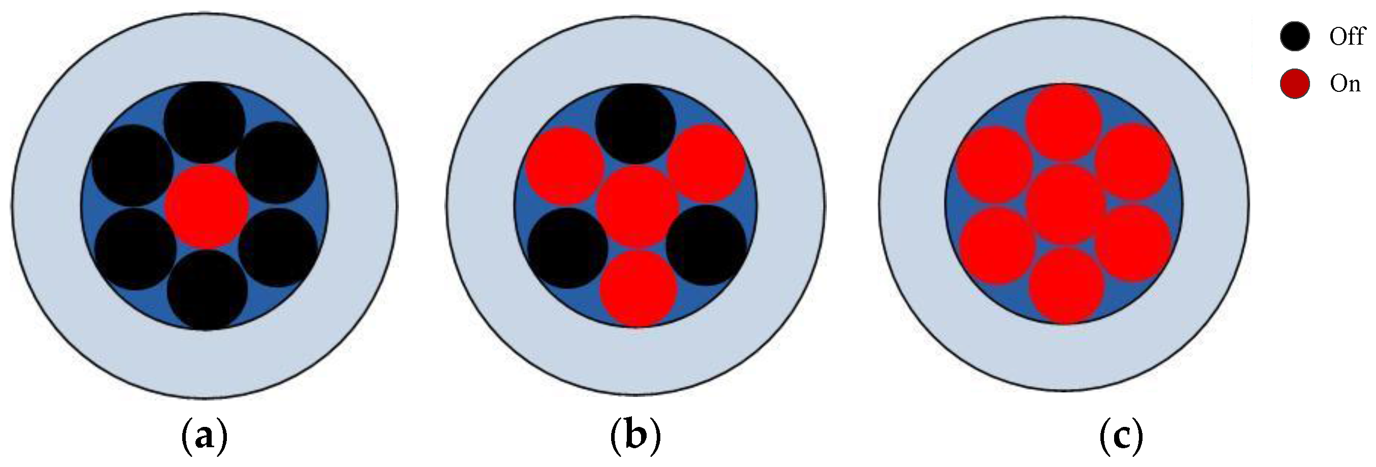
| Conduction Modes | Minimum Heating Power/W | Maximum Heating Power/W |
|---|---|---|
| Single conductor on | 25 | 900 |
| Four conductors on | 100 | 3600 |
| Seven conductors on | 170 | 6300 |
© 2016 by the authors; licensee MDPI, Basel, Switzerland. This article is an open access article distributed under the terms and conditions of the Creative Commons Attribution (CC-BY) license (http://creativecommons.org/licenses/by/4.0/).
Share and Cite
Yang, F.; Liu, K.; Cheng, P.; Wang, S.; Wang, X.; Gao, B.; Fang, Y.; Xia, R.; Ullah, I. The Coupling Fields Characteristics of Cable Joints and Application in the Evaluation of Crimping Process Defects. Energies 2016, 9, 932. https://doi.org/10.3390/en9110932
Yang F, Liu K, Cheng P, Wang S, Wang X, Gao B, Fang Y, Xia R, Ullah I. The Coupling Fields Characteristics of Cable Joints and Application in the Evaluation of Crimping Process Defects. Energies. 2016; 9(11):932. https://doi.org/10.3390/en9110932
Chicago/Turabian StyleYang, Fan, Kai Liu, Peng Cheng, Shaohua Wang, Xiaoyu Wang, Bing Gao, Yalin Fang, Rong Xia, and Irfan Ullah. 2016. "The Coupling Fields Characteristics of Cable Joints and Application in the Evaluation of Crimping Process Defects" Energies 9, no. 11: 932. https://doi.org/10.3390/en9110932
APA StyleYang, F., Liu, K., Cheng, P., Wang, S., Wang, X., Gao, B., Fang, Y., Xia, R., & Ullah, I. (2016). The Coupling Fields Characteristics of Cable Joints and Application in the Evaluation of Crimping Process Defects. Energies, 9(11), 932. https://doi.org/10.3390/en9110932