Wind Energy Assessment for Small Urban Communities in the Baja California Peninsula, Mexico

Abstract

Mexico needs to exploit its renewable resources and many studies have determined the great renewable potential it has using wind energy. However it is necessary to calculate the amount of this resource for small urban communities, which in this country lack essential services such as electricity. This study is focused in the Baja California Peninsula, using GIS as a tool to identify small urban zones with higher wind power. For this work data was analyzed from meteorological stations and recorded every 10 min for two years (2012–2014). Weibull distribution, linear regression, kriging interpolation, power and energy output and useful hours were calculated for each station. It was found that the total energy generated is 38,603,666 kWh per year and the mean of useful hours is 5220 h per year for the whole Peninsula. Maps of Wind Power Density (WPD) show a good power per square meter, GIS shows the areas with the most wind power where it can be used i.e., the state of Baja California wind power can generate electricity for 12% of those communities, meanwhile for Baja California Sur, the electric power generation could electrify almost 25% of the total of small urban communities.

1. Introduction

Developing countries face different problems; one of them is electricity, correlating with better education, social security and health services. In Mexico, dependence in crude oil generates economic problems however, with the structural reforms done by government RES could have less dependence on crude oil [1]. According to the World Bank, Mexico has 62% of its rural population in poverty, but its access to electricity is 97.2%, while urban population access to electricity is 99.6% [2]. Its electricity production from coal represents 11%, oil 16%, gas 56%, nuclear 4%, hydroelectric 9%, geothermal 2% and wind 1% and other sources 0.5% [3]. By Renewable Energy Sources (RES) wind energy and solar energy increased in 2013, 53.6% and 15% respectively, meanwhile biogas and geothermic energy decreased 1.6% and 1.1% respectively [4]. In 2008, the Mexican government reformed its energy law which would open the electricity sector to the private market, currently CFE (which is the government office of electricity and still controlling the Mexican power market to transmit, distribute and supply energy [5]), established that in 2018, 2021 and 2024, the 25%, 30% and 35% respectively, the electric generation will come from RES [6]. Wind power generation in Mexico has grown slowly, although the cost of the wind turbines has declined largely due to technological development, which has been an incentive for the development of renewable energy. [7] indicates that manufacturers of wind turbines have reduced the cost of generation by implementing new manufacturing techniques using best engineering tools, as well as improving design, which provides a technological challenge to achieve a greater amount of wind power and increased system reliability, in order to deliver to the consumer, or customer, a price that competes with other forms of conventional energy production. In 1994 a study was conducted to electrify the remote village of San Antonio Agua Bendita using a custom designed hybrid power system. This study provided 120 VAC power at 60 Hz. to anticipated industrial loads in the village, as well as providing grid quality power for domestic use [8]. The Mexican government launched a solar PV program in 1998 for over 1250 small urban communities of almost 200,000 people, based mostly on solar home systems due to the large population dispersion [9]. Electricity in Mexico is supplied by the Federal Commission of Electricity (CFE) utility owned by government. In April 2015 they proposed the Expansion and Modernization Program of the main grid distribution 2015–2019, this program establishing that in 2014, the 94.87% of small urban population should have electricity and its aim was to electrify the remaining 5.13% [10]. In Mexico, while a variety of biomass fuels exists, firewood represents the dominant form of traditional energy in small urban [11], and the use of electricity in municipal services (street lighting, water pumping and public buildings) has become a major economic burden on municipalities, due to the tariff regime to which they are subjected to. In many cases, power consumption represents a high percentage of total operating expenses of a municipality, creating a drag on development. Indeed, the possibility of an alternative supply to the utility has led some municipalities to accept, or to take initiatives to develop self-supply projects that allow them to have electricity at a lower price fixing tariffs. According to [12], the latest government program established from 2002 to 2007 was to provide renewable electricity to 50,000 in 2500 marginalized small urban communities in the states of Chiapas, Guerrero, Oaxaca and Veracruz. Geographic Information System (GIS) have been successfully employed to locate geographical areas with suitable potential for cultivating renewable energies: wind power [13,14,15,16,17], biomass [18,19,20,21,22,23,24] or solar [25,26,27,28,29]. Some urban assessment has been done by some authors [30] and examined the capacity and energy output of RES available, area-based on constraints such as land use and altitude; methodology to find seasonal irradiation, wind speed, biomass and small hydropower capacity was developed by [31]; to examine wind as renewable source using GIS a quantitative index has been proposed by [32]. A study showed wind effects into urban areas and found that wind speed at observation stations decreases due to the drag effect of buildings [33].

The main aim of this study is to assess wind energy potential for rural electrification at the Baja California Peninsula, Mexico, to establish the amount of electrical energy provided to these communities and GIS will indicate the areas where wind resource is higher.

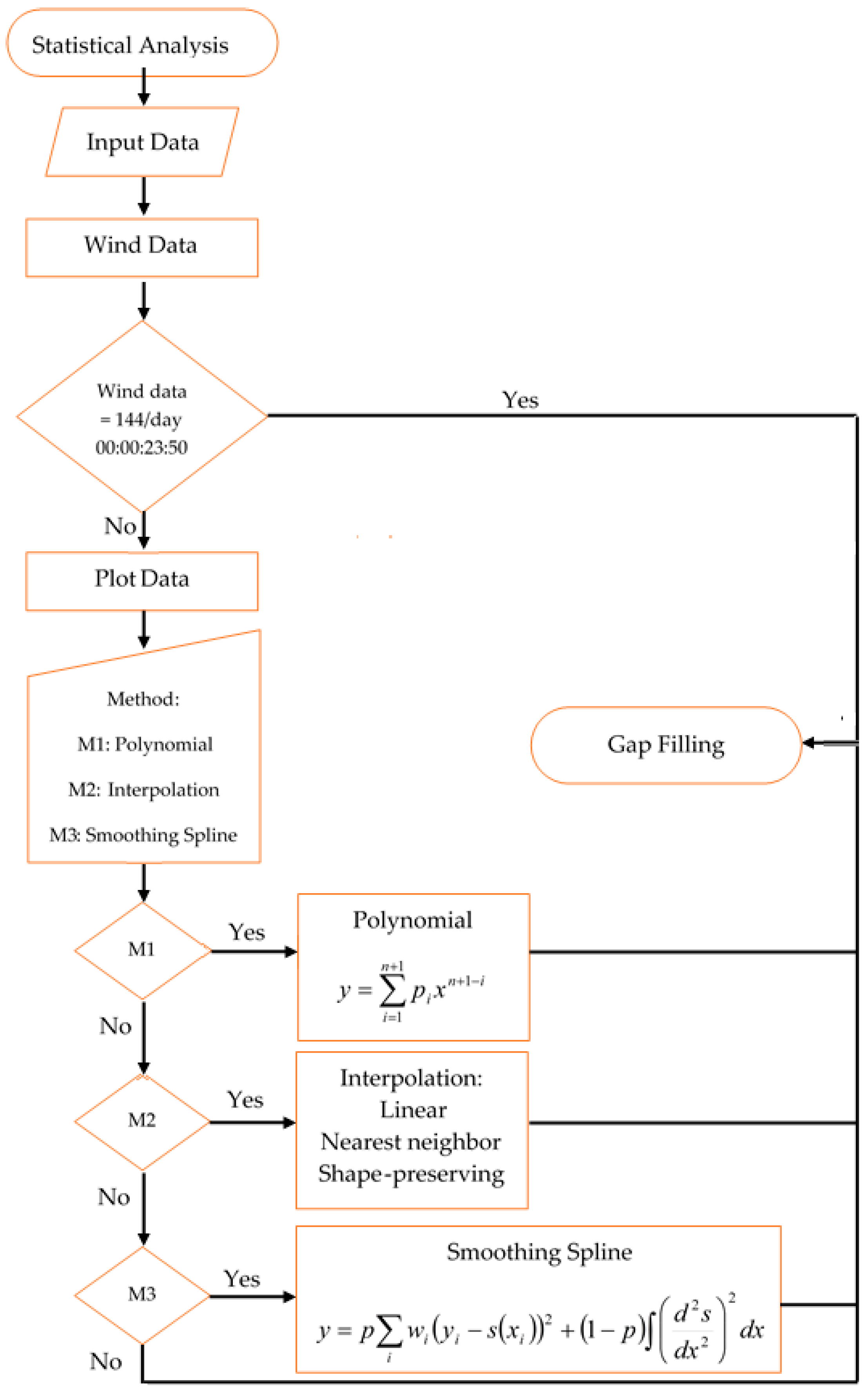
2. Materials and Methods

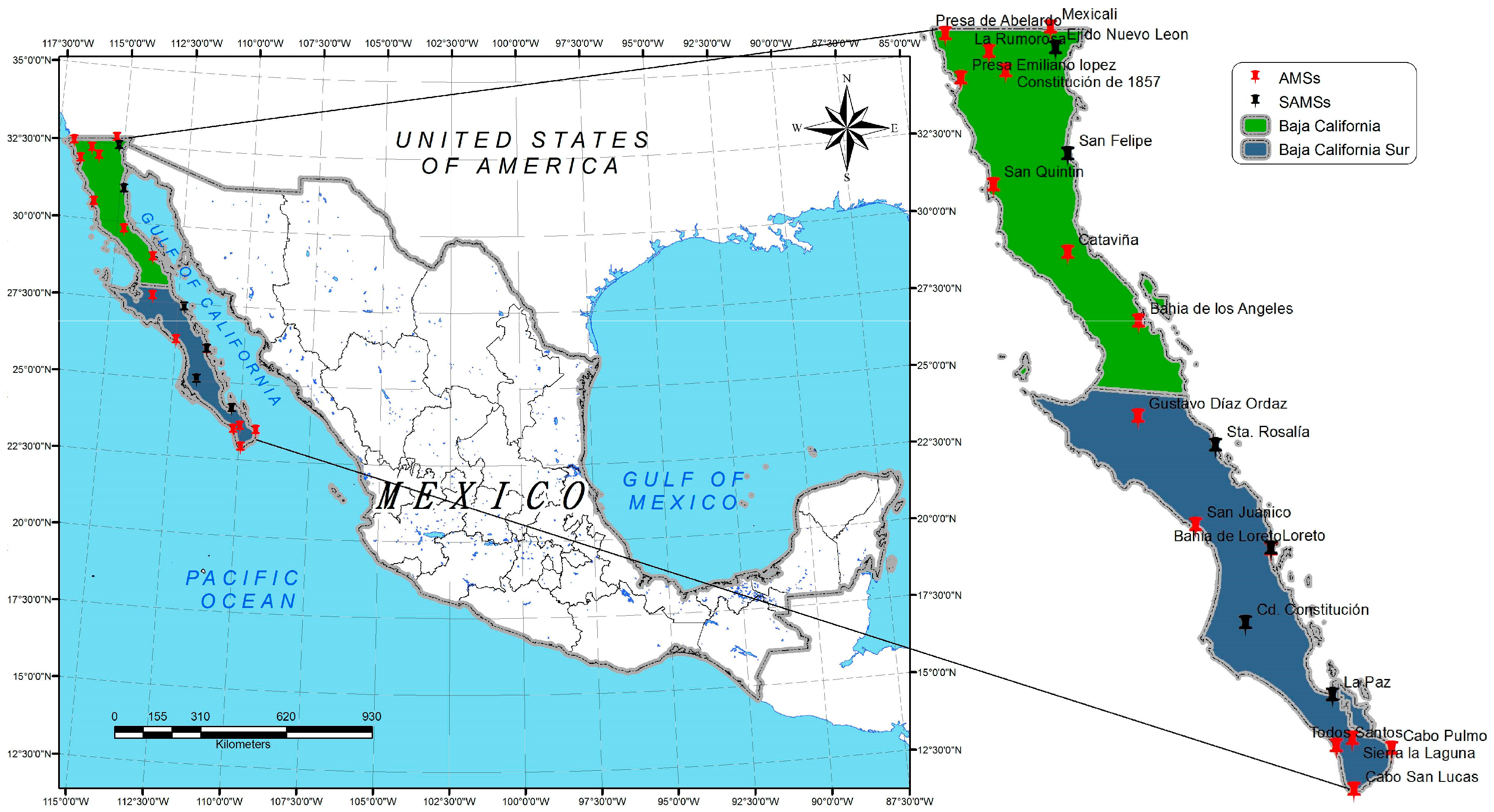
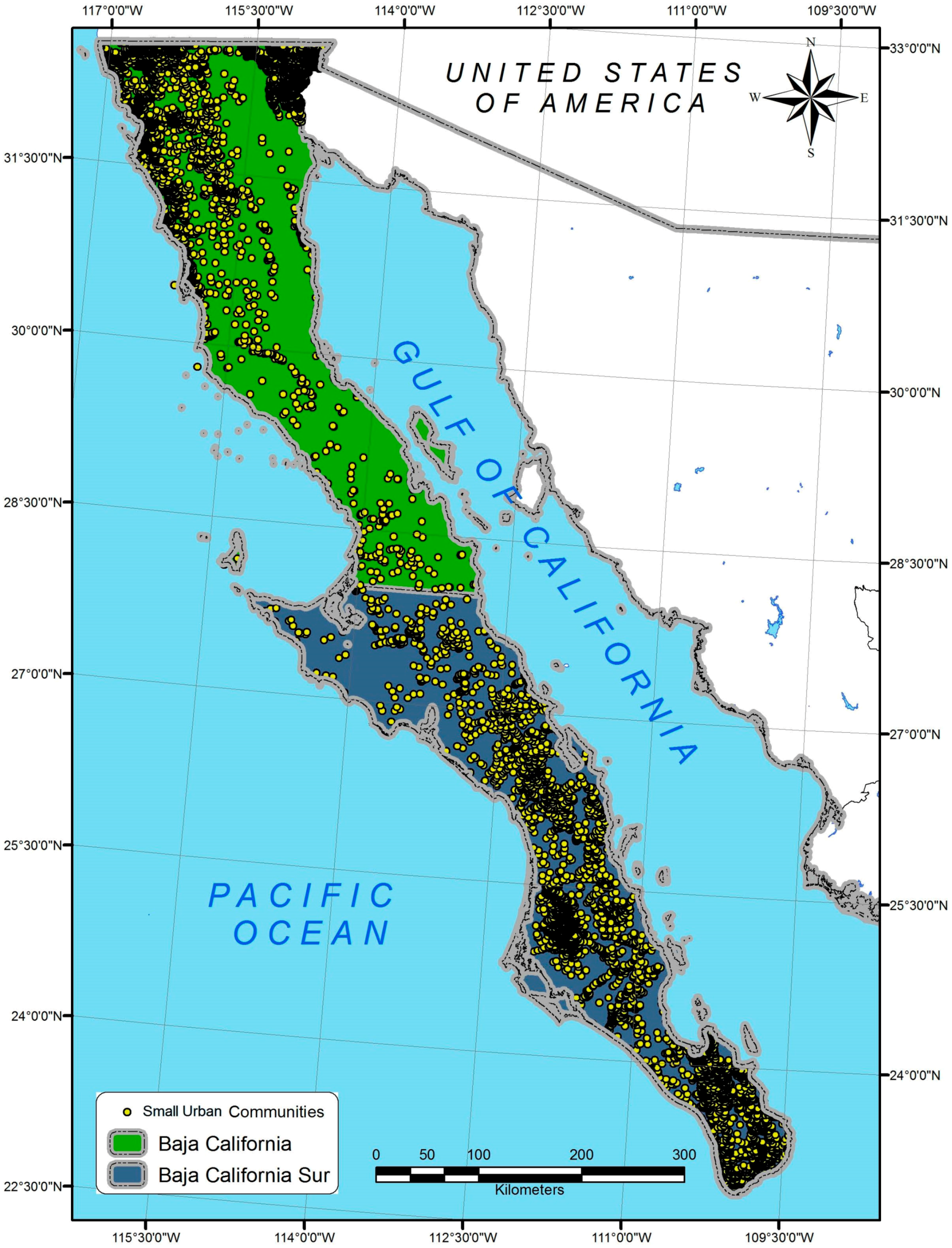
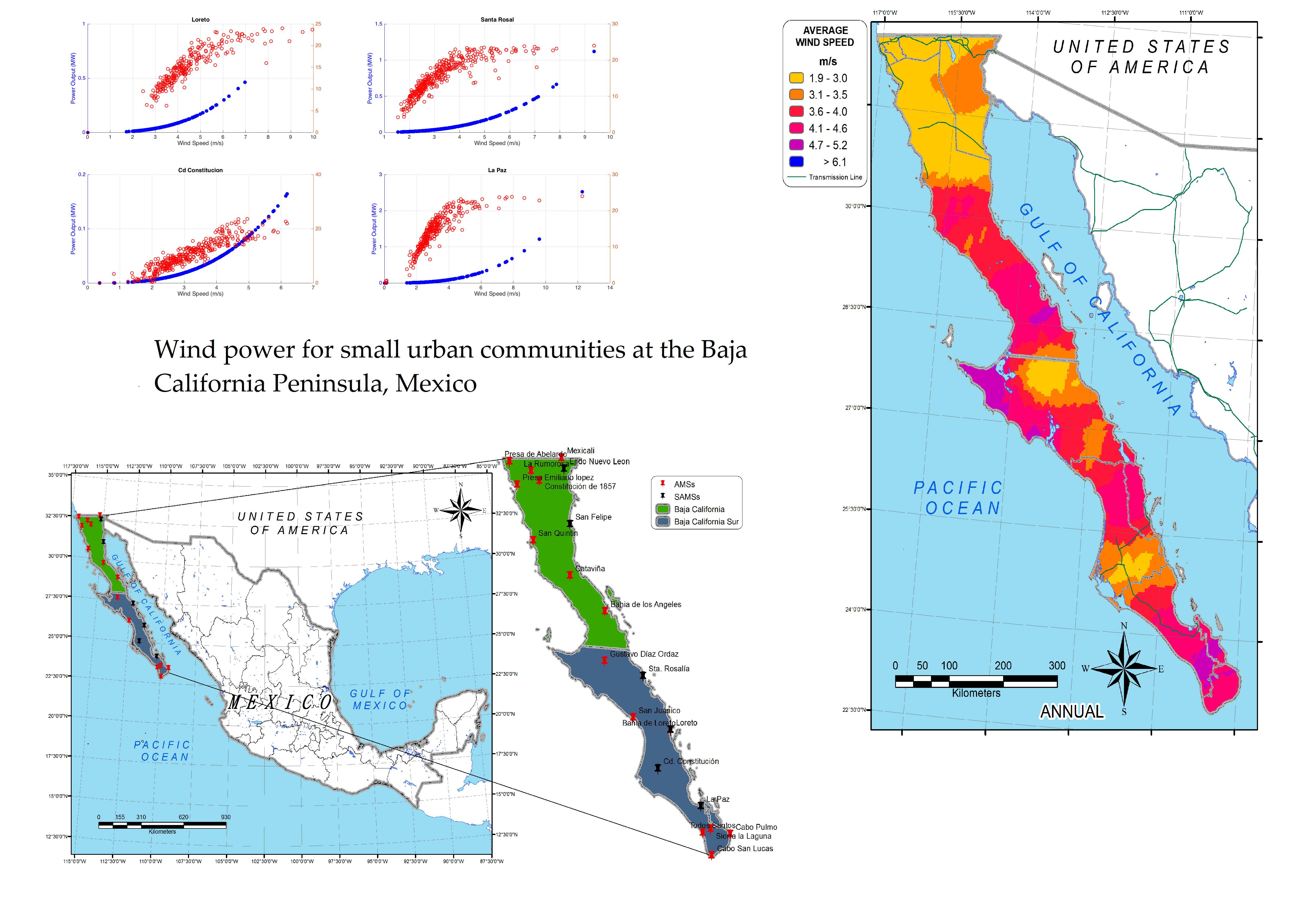
Some small urban communities in Mexico are in isolated areas, without the essential services such as roads and electricity. The Baja California Peninsula consists of two states, Baja California and Baja California Sur, the first having 3,155,070 people; around 853,254 households in which 98.5% have electricity and its small urban population is 8%. Baja California Sur has 637,026 people, 174,441 households, 96.7% of them having electricity and 14% is its small urban population [34].

2.1. Data

In spite of the ever-increasing network of meteorological stations around the world, the availability of solar radiation data is still limited for many applications in terms of spatial distribution [35]. Consequently, it is widely accepted that global solar radiation data derived from satellites are an excellent tool for analyzing solar resources and for supplying time series of solar irradiation [36,37]. This application was demonstrated by Pedro and Coimbra [38], who evaluated techniques to prognosticate solar potential using nonexogenous data. Wind assessment [16] demonstrated data validation between recorded and satellite data, showing that it could get 98% of correlation between these variables.

Data recorded from 2012 to 2014, every 10 min, were extracted from 17 Automatic Meteorological Stations (AMSs) and 7 Synoptic Automatic Meteorological Stations (SAMSs) from National Meteorological Service of Mexico (NMS) [39] and extrapolated at a height of 50 m. An AMS and SAMS, consists of a group of sensors that record and transmit weather information automatically from the areas where they are strategically placed. Its main function is the collection and monitoring of meteorological variables such as wind direction and speed and generates files on an average of every 10 min of all the variables. This information is then sent via satellite at intervals of 1 or 3 h per meteorological station and data is gathered at 80 points by means of monthly recordings obtained over a period of 22 years up to 2014, taken by the Surface Meteorology and Solar Energy (SMSE) who described that data was obtained from the NASA Science Mission Directorate’s satellite and re-analysis research programs. Parameters based upon the solar and/or meteorology data were derived and validated based on recommendations from partners in the energy industry. This source is from the Atmospheric Science Data Center (ASDC) from NASA at a height of 50 m, data which was also used [40].

Data treatments were made for whole data series, first of all establishing missing data, to fill gaps an application was developed, then an interpolation model calculated and applied it to the data time series, i.e., the AMSs Bahia Los Angeles, January 2012. This application finds missing data, comparing the hour and day and separates them, then runs an interpolation model and finally calculates the missing data. This method completes a time series, Figure 1 shows schematically this algorithm. To determine data quality has been calculated the correlation coefficient, Root Mean Square Error (RMSE), Bias, SD and R-Square between AMSs vs. SAMSs vs. SMSE.

Table 1. Number of meteorological stations and SMSE points along the Baja California Peninsula.

State	Source
	AMSs	SAMSs	SMSE
Baja California	10	3	25
Baja California Sur	7	4	55

show the number of meteorological stations and points selected from SMSE on the Baja California Peninsula.

Figure 2 shows the geographic position of AMSs, SAMSs on the Baja California Peninsula, Mexico.

There are around 2500 small urban communities on the Peninsula and are distributed as shown in Figure 2. It can be observed that they are concentrated in the north, next to the US border, meanwhile in the state of Baja California Sur, the small urban communities are extended along its length.

Linear Regression Data at the Baja California Peninsula

Linear Regression is commonly used in wind speed assessment, because it is a rather simple and relievable method. In this work, it is used to fit linearly AMSs vs. SMSE and SAMs vs. SMSE data where a linear function is fitted to the available data according to Equation (1).

$$y=\mathsf{\alpha }+\mathsf{\beta }x$$

(1)

Parameter α and β can be determine by setting wind speed from reference data as x-values and measured data as y-values, expressed in Equation (2).

$$\mathsf{\beta }=\frac{{\displaystyle \sum _{i=1}^n{x}_i{y}_i-\frac{{\displaystyle \sum _{i=1}^n{x}_i}{\displaystyle \sum _{i=1}^n{y}_i}}{n}}}{{\displaystyle \sum _{i=1}^n{x}_i^2-\frac{{\left({\displaystyle \sum _{i=1}^n{x}_i}\right)}^2}{n}}}$$

(2)

RMSE accordingly [41] can be expressed in terms of bias and the variance of error, these variables would use to calculate the error between AMSs, SAMSs vs. SMSE.

As shown in Figure 3 the small urban communities are distributed through the Baja California Peninsula, however in the north of Baja California State most of the cities are concentrated, by other hand in Baja California Sur cities are settled down along it.

2.2. Wind Assessment at Baja California Peninsula

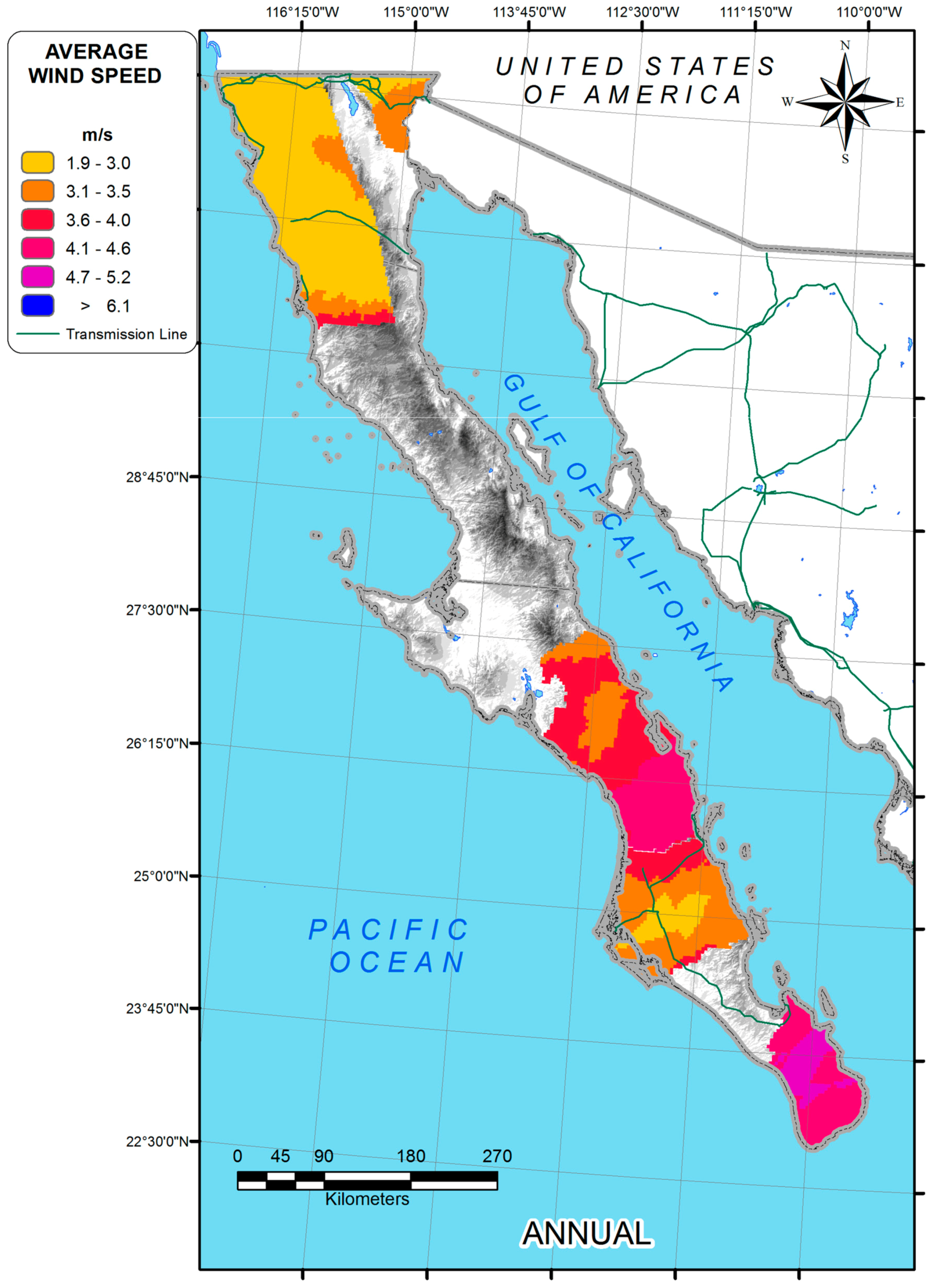
2.2.1. Wind Speed

The Baja California Peninsula presents a good wind regime. In 2004 a study was done by [42] and established that in Baja California Sur, specifically in El Cardon, wind power could be around 700 kW, even in this study there is not an assessment for small urban communities. For each selected site, a complete five-year data recording was extracted.

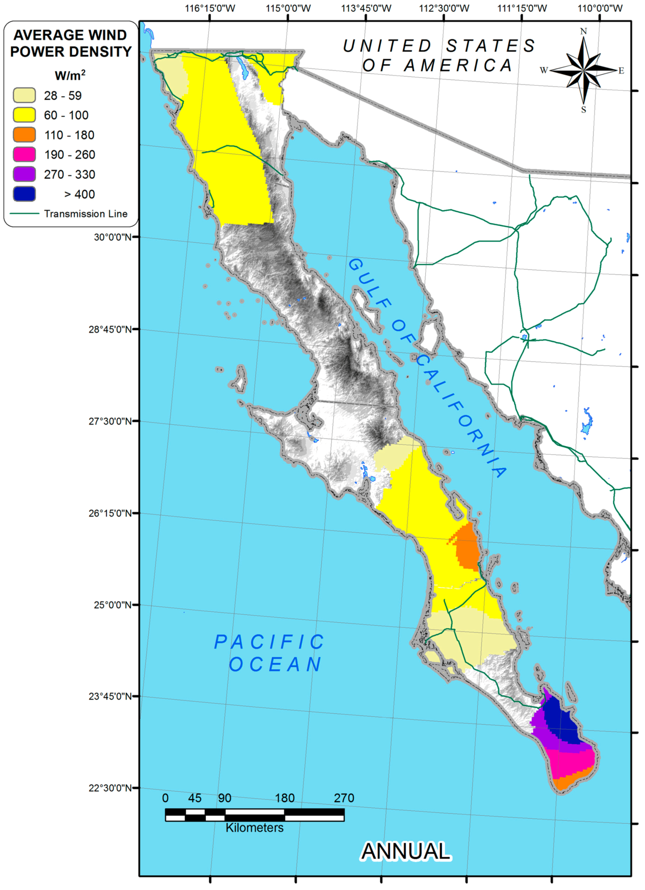
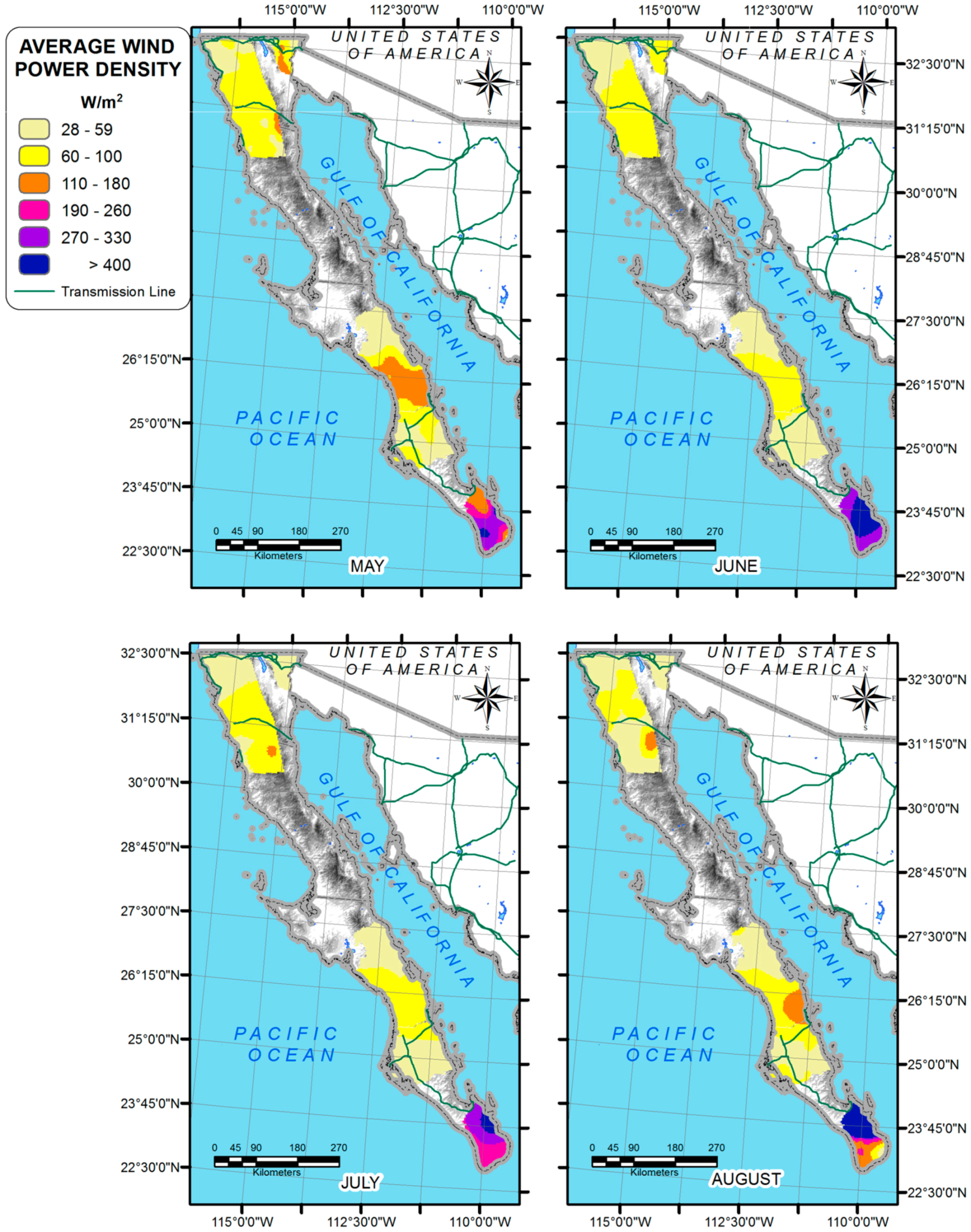
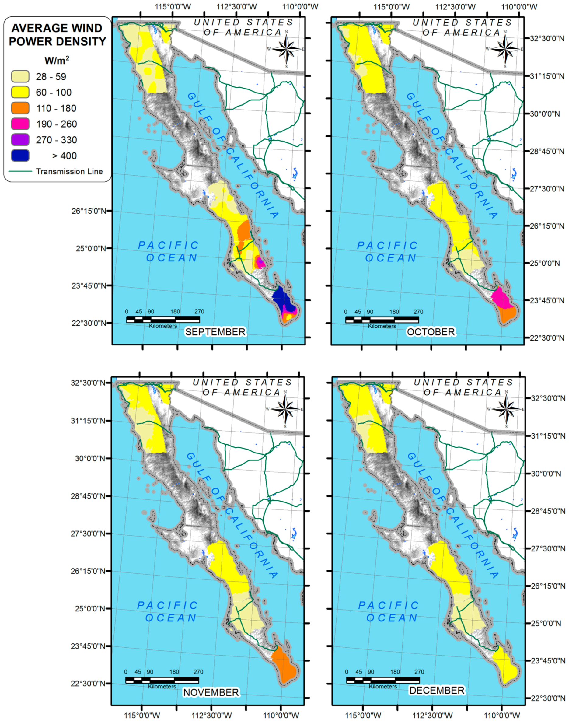
2.2.2. Wind Power Density

The frequency of occurrence of wind speeds may be described by the probability density function, p(U), of wind speed. In Equation (3), the probability density function may be used to express the probability of a wind speed occurring between Ua and Ub:

$$p\left(U_a\le U\le U_b\right)={\displaystyle \underset{U_a}{\overset{U_b}{\int }}p\left(U\right)dU}$$

(3)

Also total area under the probability density curve is given by Equation (4).

$${\displaystyle \underset{0}{\overset{\infty }{\int }}p\left(U\right)dU=1}$$

(4)

If p(U) I known, the parameters can be calculated, mean wind speed, $\overline{U}$, Equation (5).

$$\overline{U}={\displaystyle {\int }_0^{\infty }Up\left(U\right)dU}$$

(5)

Standard deviation of wind speed, σ_U, it is defined by Equation (6).

$${\mathsf{\sigma }}_U=\sqrt{{\displaystyle \underset{0}{\overset{\infty }{\int }}{\left(U-\overline{U}\right)}^{2}p\left(U\right)dU}}$$

(6)

Equation (7) shows the mean available WPD $\overline{P}/A$ [43].

$$\raisebox{1ex}{$\overline{P}$}\!\left/ \!\raisebox{-1ex}{$A$}\right.=\left(1/2\right)\mathsf{\rho }{\displaystyle \underset{0}{\overset{\infty }{\int }}{U}^{3}p\left(U\right)dU=\left(1/2\right)\mathsf{\rho }\overline{U^3}}$$

(7)

2.2.3. Weibull Distribution

The Weibull distribution provides a close approximation to the probability laws of many natural phenomena. It has been used to represent wind speed distributions for application in wind loads studies for sometime [42]. Two probability distribution functions are commonly used for wind speed. The simpler of the two is the Rayleigh distribution, which has a single parameter c and velocity of the wind (V), see Equation (8).

$$f(V)=\frac{2V}{c^2}{e}^{-{\left(V/c\right)}^2}0\le \mathrm{V}<\infty$$

(8)

The Weibull distribution has a parameter k called shape parameter and parameter c scale parameter, k describes the variability about the mean and c is related to the annual mean wind speed as seen in Equation (9).

$$f(V)=\frac{k}{c}{\left(\frac{V}{c}\right)}^{k-1}{e}^{-{\left(V/c\right)}^k}0\le V<\infty$$

(9)

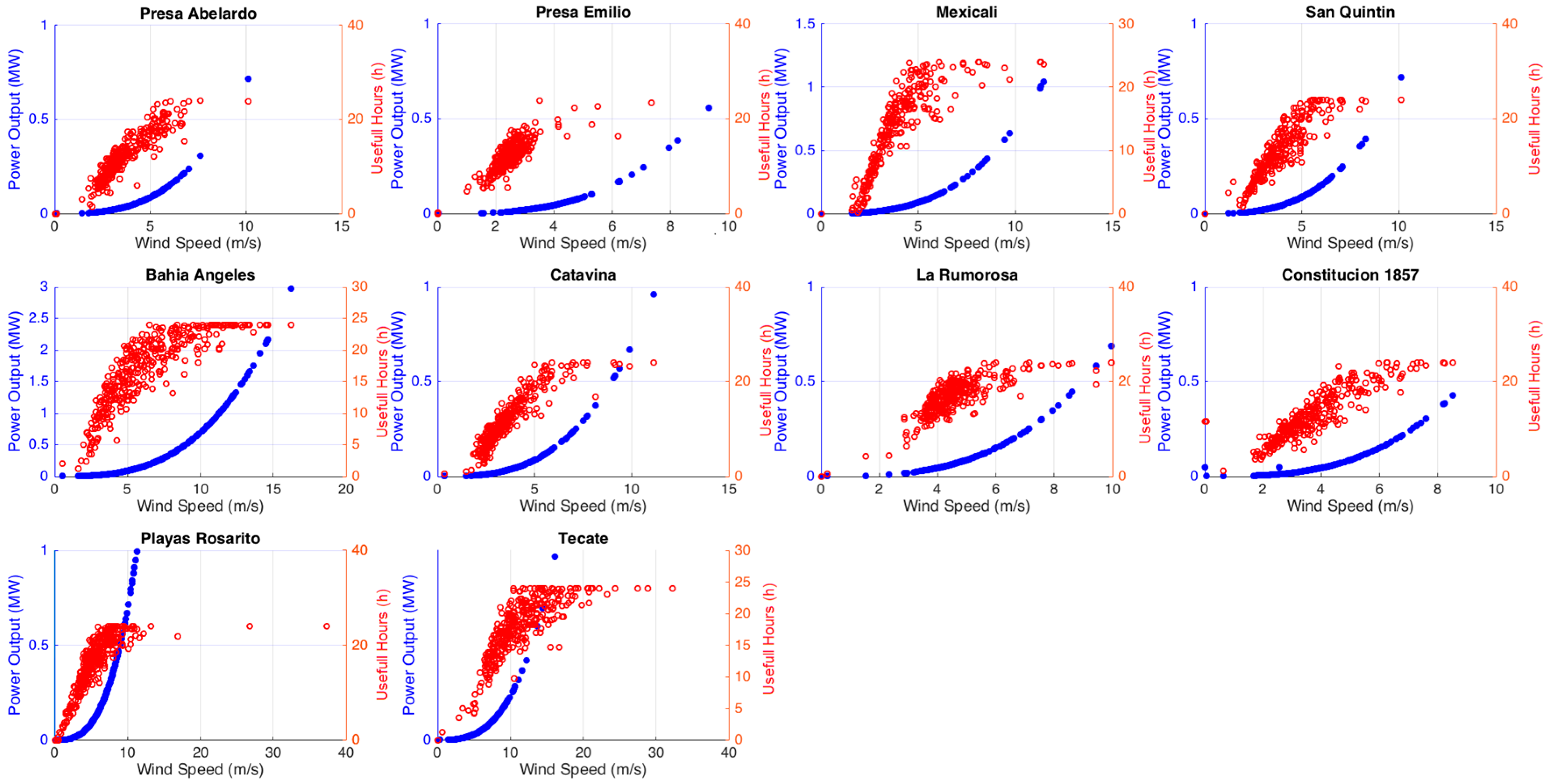
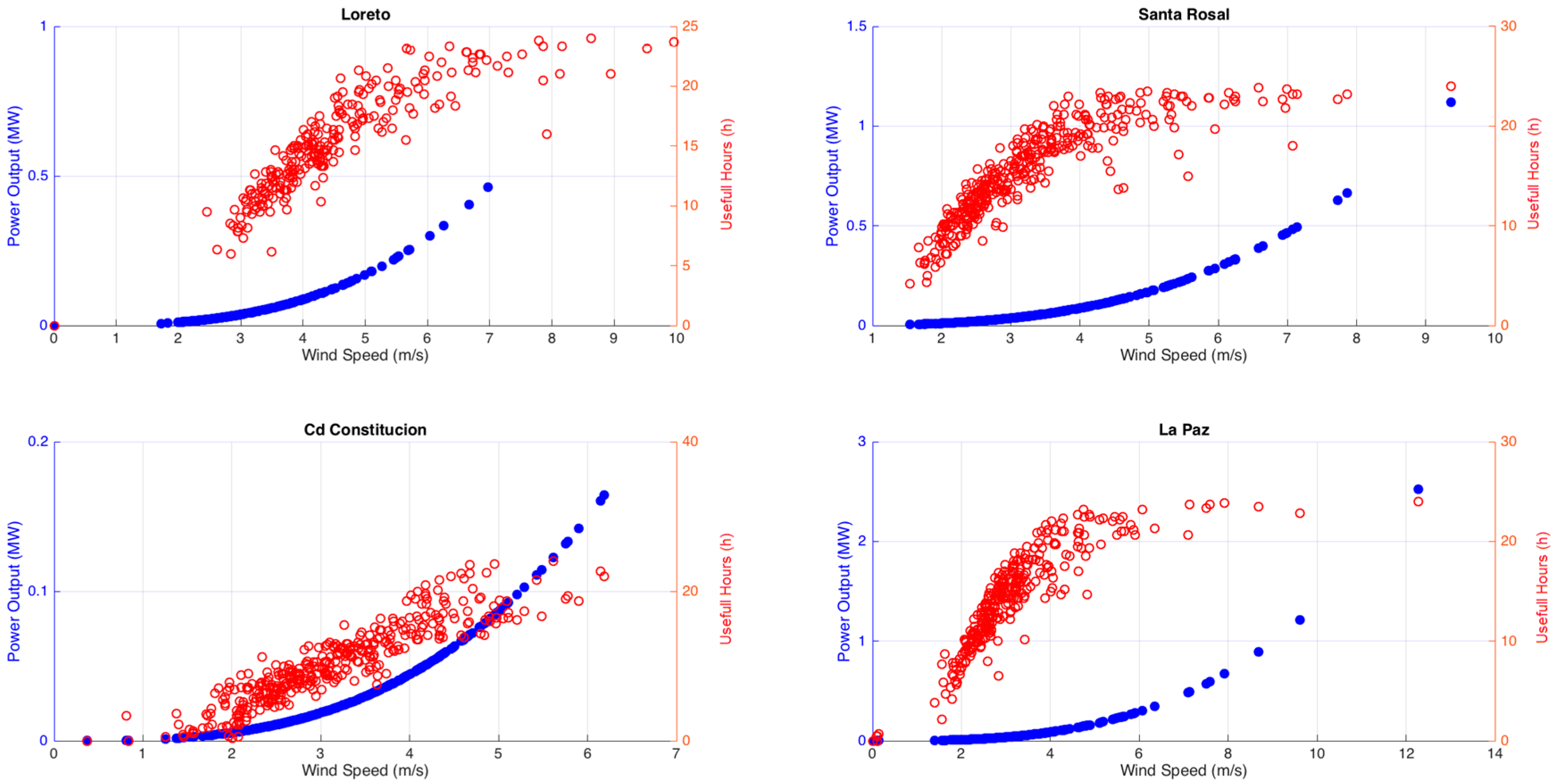
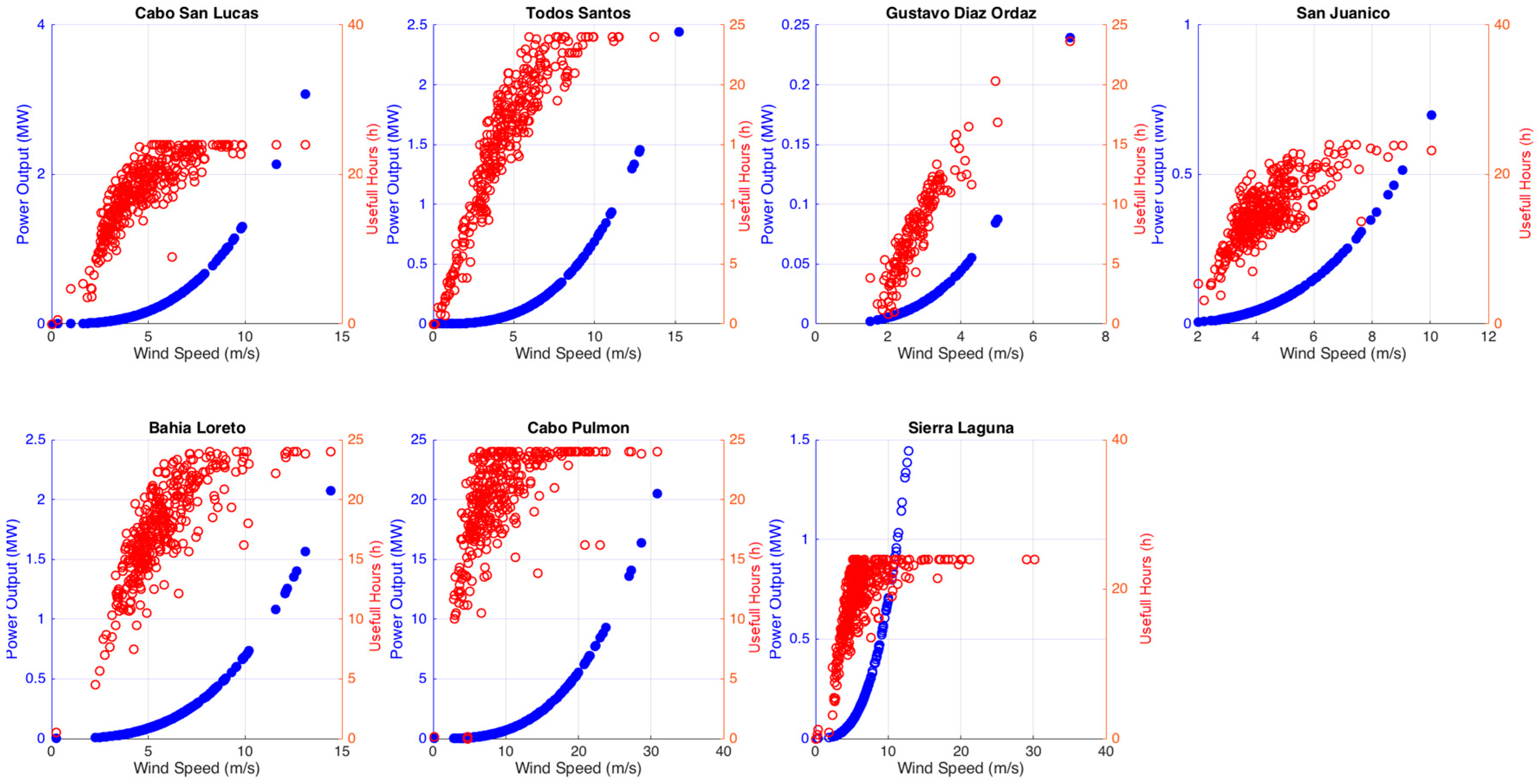
2.2.4. Power and Energy Output

Data were extrapolated at the 50 m height so the magnitude of power output at different hub heights could be calculated, it was important to assume that the gross turbine power output depends on three factors: the turbine’s power curve, the wind speed at hub height and the air density. For a stall-controlled wind turbine, the power output predicted by the power curve for the measured wind speed must be calculated and then adjustments made to the power output, according to the Equation (10).

$$P=P_0\frac{\mathsf{\rho }}{{\mathsf{\rho }}_0}$$

(10)

where, P₀ is the power output predicted by the power curve for the wind speed in the current time step (kW), ρ is the actual air density in the current time step (kg/m³), ρ₀ is the air density at which the power curve applies (kg/m³).

The mean net power output can be calculated using Equation (11), this equation takes the mean gross power output for each month and the gross power output of the wind turbine in each time step.

$${\overline{P}}_{net}=\left(1-f_{overall}\right){\overline{P}}_{gross}$$

(11)

where, P_gross is the mean gross power output before losses [kW] and f_overall is the overall loss factor.

The mean net power output for each month of the year and for the entire data set were used to find the mean net energy, it multiplied these values of mean net power output by the appropriate number of useful hours in order to find the turbine’s annual output, Equation (12).

$$E_{net,annual}={\overline{P}}_{net,overall}·8760h$$

(12)

2.2.5. Useful Hours

The mean net energy output must be calculated, multiplying by the useful hours of wind speed; this amount of useful hours is calculated excluding the time series of wind speed above 2.5 m/s during a day.

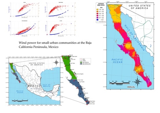
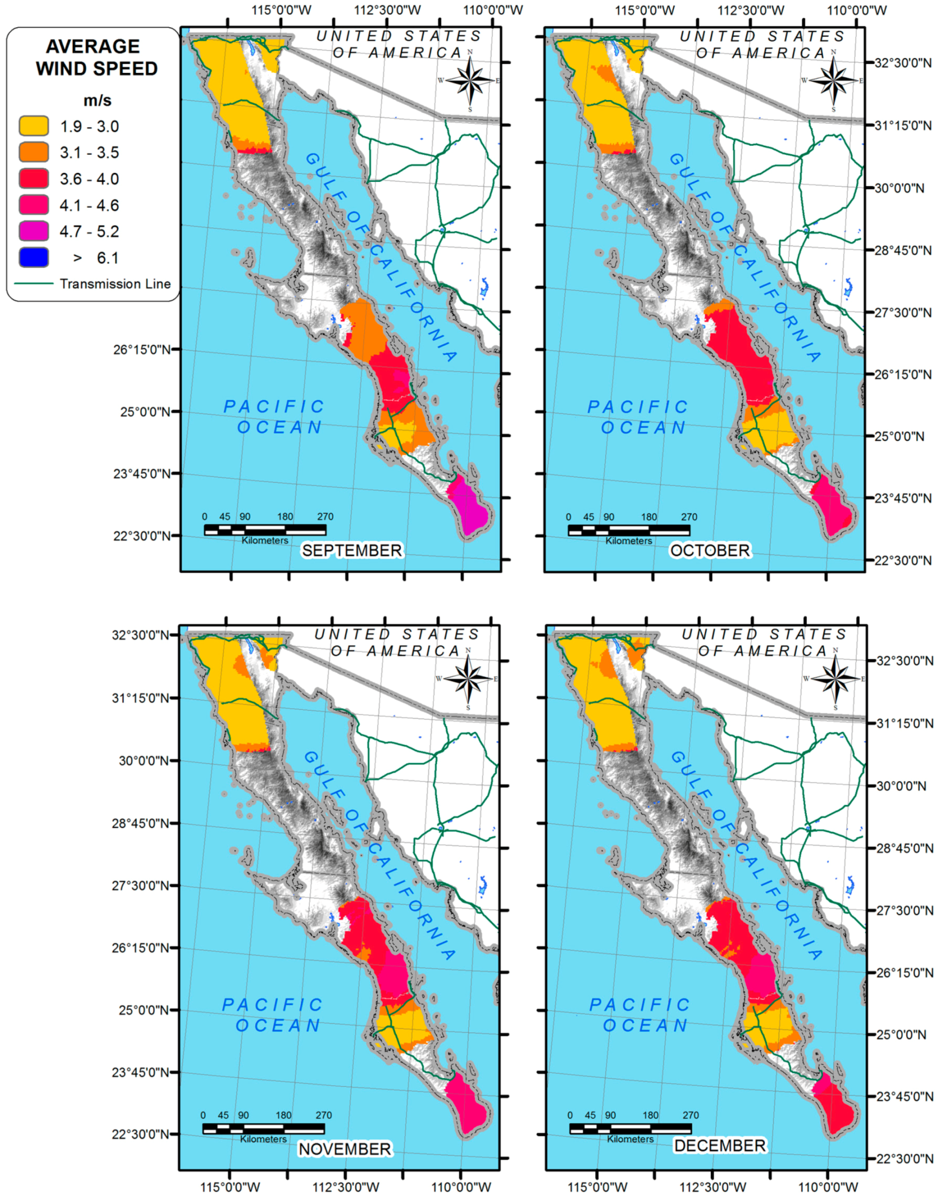
2.3. Wind Speed and WPD Maps GIS-Based

In general, GIS can represent both wind speed and WPD, however GIS displays a spatial interpolation because does not consider any topography in this case, small urban communities were considered without roughness due to the topography of these areas.

Kriging estimators [44] belong to the class of the Best Linear Unblased Estimators (BLUE). Kriging are minimum variance estimators and yield, within the class of the linear estimators. Two of the most used Kriging models are the Ordinary Kriging (OK) and Universal Kriging (UK). The basis of the hypothesis in the UK is that is it possible to write the trend function as a linear combination of elementary functions, which are generally monomial. The weights of this combination are called drift coefficients. The UK yields their estimates with the minimum overall variance of the combined estimate of the trend function and of the small scale variability. Data was interpolated using the Kriging method from ArcGIS v10.2 and this method assumes that the distance, or direction between the sample points, reflects a spatial correlation.

3. Results

3.1. Data Validation

Data analysis is the basis for investigations in wind speed assessment, most of the data fulfilled the control procedures, however, data from certain stations was removed. Next, the stability of wind speed was assessed through statistical analyses. Data from AMSs and SAMSs are named as fixed sensors, to correlate SMSE vs. AMSs and SAMSs data, there was a consideration, SMSE location were selected at the same position as AMSs or SAMSs. Input data as well as fixed sensor as satellite are monthly data during a year.

R-square identifies the linear fit between two variables, in this case AMSs and SMSE, or SAMSs and SMSE data were aligned, the values registered having a range of 0.61 to 0.96. San Quintin has a R-square of 0.96, Bias = 0.258, SD = 0.451 and RMSE = 0.07969. The lower value La Rumorosa has a R-square of 0.61, Bias = −0.065, SD = 0.533 and RMSE = 0.3052; even though R-Square is low, Bias, SD and RMSE are close to 0 which means the fit has few errors between data, see

Table 2. R-Square, Bias and RMSE of AMSs, SAMSs vs SMSE Data.

State	Source	Meteorological Station	R-Square (%)	SD (σ)	Bias (m/s)	RMSE (m/s)	Source
Baja California	AMSs	Presa_Abel	0.84	0.296	−0.039	0.1559	SMSE_1
Baja California	AMSs	Presa_Emilio	0.94	0.341	0.366	0.09359	SMSE_2
Baja California	AMSs	Mexicali	0.79	0.331	0.226	0.1793	SMSE_3
Baja California	AMSs	San Quintin	0.96	0.451	0.258	0.07969	SMSE_4
Baja California	AMSs	Bahia Ange	0.77	0.415	−0.041	0.1851	SMSE_5
Baja California	AMSs	Catavina	0.77	0.528	0.268	0.1889	SMSE_8
Baja California	AMSs	La_Rumorosa	0.61	0.533	−0.065	0.3052	SMSE_9
Baja California	AMSs	Cons_1857	0.70	0.423	−0.167	0.2684	SMSE_10
Baja California	AMSs	Playas_Rosa	0.71	0.452	0.129	0.265	SMSE_11
Baja California	AMSs	Tecate	0.62	0.390	0.468	0.3203	SMSE_14
Baja California Sur	AMSs	Todos_Santos	0.72	0.555	0.057	0.283	SMSE_12
Baja California Sur	AMSs	Cabo_SanLucas	0.74	0.325	0.307	0.2564	SMSE_15
Baja California Sur	AMSs	Gust_Diaz_O	0.71	0.412	0.617	0.2709	SMSE_16
Baja California Sur	AMSs	San_Juanico	0.88	0.549	0.006	0.1433	SMSE_17
Baja California Sur	AMSs	Bahia_Loreto	0.81	0.475	0.089	0.1794	SMSE_18
Baja California Sur	AMSs	Cabo_Pulmon	0.86	0.806	0.054	0.199	SMSE_19
Baja California Sur	AMSs	Sierra_Laguna	0.83	0.733	0.173	0.2028	SMSE_20
Baja California	SAMSs	San Felipe	0.72	0.706	0.116	0.2918	SMSE_21
Baja California	SAMSs	Ejido_Nleon	0.63	0.657	0.656	0.3298	SMSE_22
Baja California	SAMSs	Algodones	0.84	0.504	0.231	0.1742	SMSE_25
Baja California Sur	SAMSs	Loreto	0.79	0.322	−0.002	0.2872	SMSE_23
Baja California Sur	SAMSs	Santa_Rosa	0.73	0.307	0.099	0.184	SMSE_24
Baja California Sur	SAMSs	Cd_Consti	0.85	0.522	−0.077	0.1698	SMSE_30
Baja California Sur	SAMSs	La Paz	0.72	0.474	−0.615	0.2158	SMSE_31

.

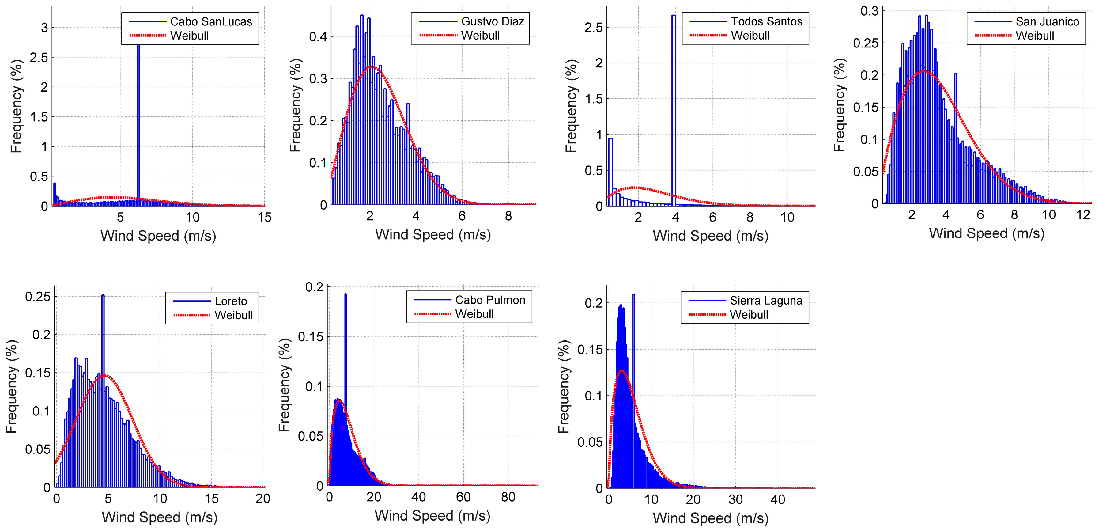
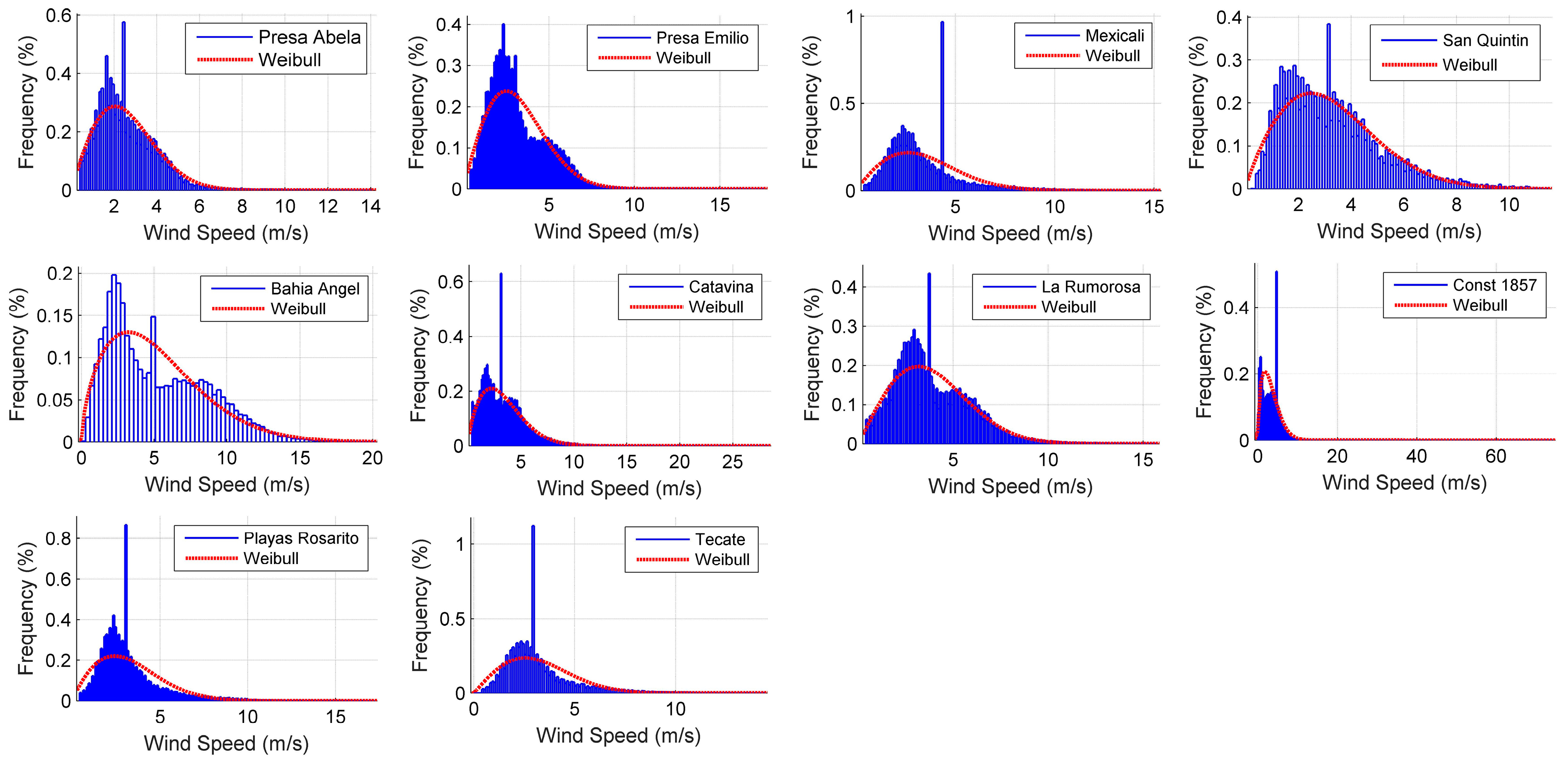
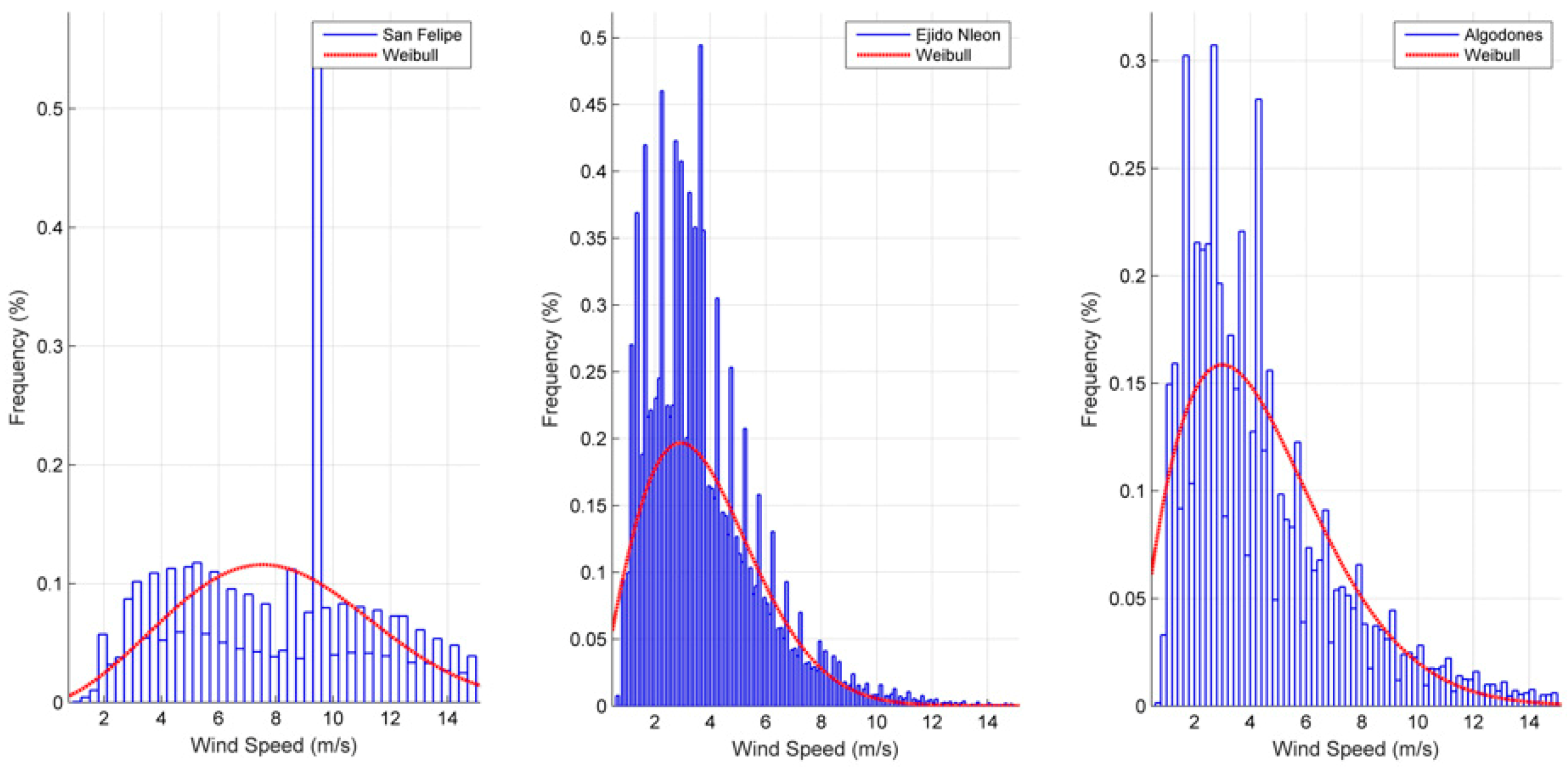
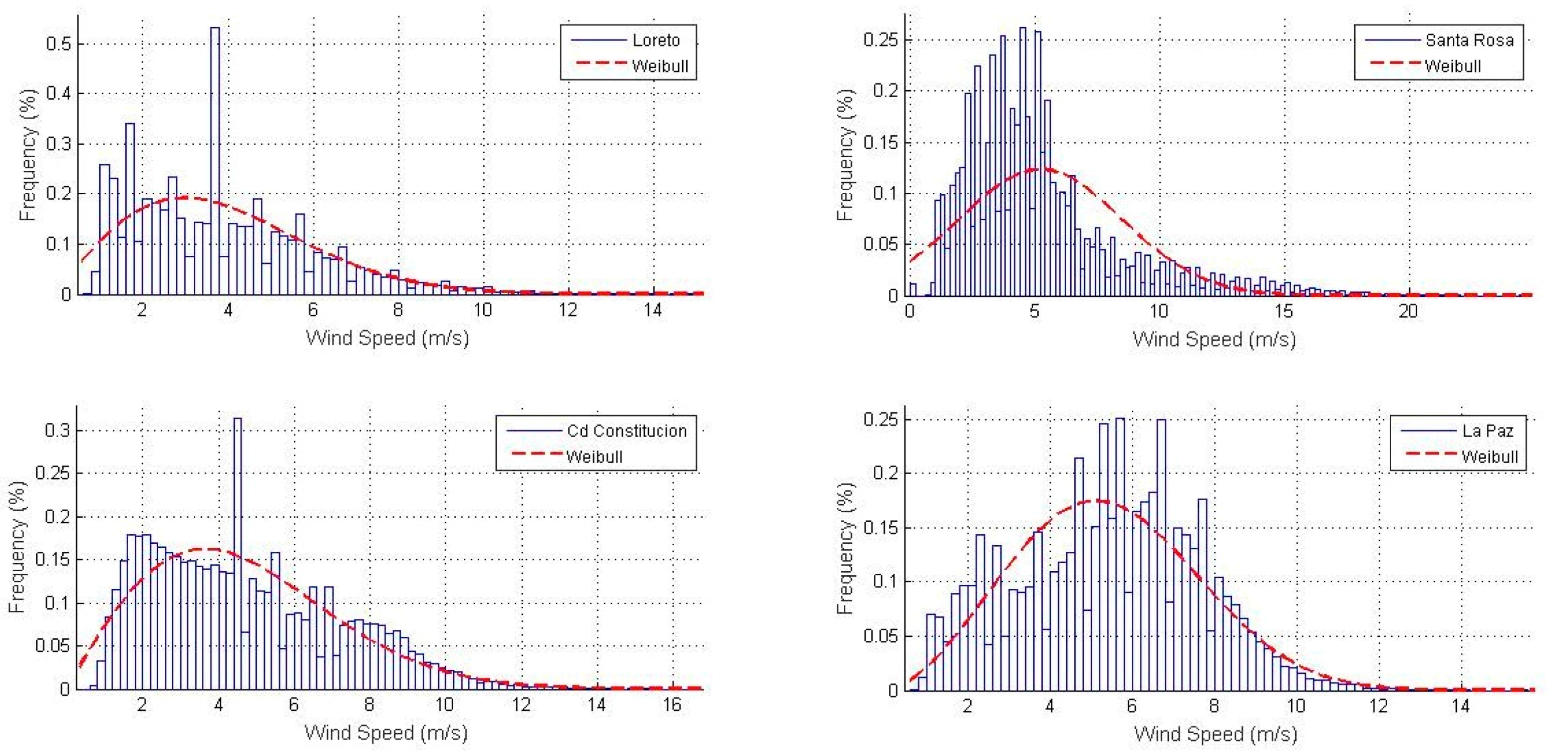
3.2. Weibull Distribution

Weibull parameters k and c were calculated for 24 meteorological stations along the Baja California Peninsula,

Table 3. Weibull Parameters of AMSs and SAMSs at the Baja California Peninsula.

State	Source	Met Station		Weibull Parameters
			Mean	k	c
			(m/s)	Dimensionless	(m/s)
Baja California	AMSs	Presa_Abel	2.61	1.96	2.94
Baja California	AMSs	Presa_Emilio	3.18	1.98	3.58
Baja California	AMSs	Mexicali	3.40	1.92	3.83
Baja California	AMSs	San Quintin	3.29	1.88	3.71
Baja California	AMSs	Bahia Ange	5.25	1.23	5.86
Baja California	AMSs	Catavina	3.32	1.70	3.73
Baja California	AMSs	La_Rumorosa	3.90	2.05	4.41
Baja California	AMSs	Cons_1857	3.22	1.53	3.57
Baja California	AMSs	Playas_Rosa	3.27	1.84	3.68
Baja California	AMSs	Tecate	3.21	1.99	3.62
Baja California Sur	AMSs	Todos_Santos	2.70	1.68	3.03
Baja California Sur	AMSs	Cabo_SanLucas	5.36	2.08	6.06
Baja California Sur	AMSs	Gust_Diaz_O	2.45	2.17	2.76
Baja California Sur	AMSs	San_Juanico	3.55	1.88	4.00
Baja California Sur	AMSs	Bahia_Loreto	4.63	1.72	4.63
Baja California Sur	AMSs	Cabo_Pulmon	7.89	1.55	8.77
Baja California Sur	AMSs	Sierra_Laguna	5.32	1.55	5.92
Baja California	SAMSs	San Felipe	8.04	2.62	9.05
Baja California	SAMSs	Ejido_Nleon	3.78	1.93	4.26
Baja California	SAMSs	Algodones	4.42	1.72	4.96
Baja California Sur	SAMSs	Loreto	3.88	1.93	4.37
Baja California Sur	SAMSs	Santa_Rosa	5.22	1.62	5.22
Baja California Sur	SAMSs	Cd_Consti	4.65	1.97	5.24
Baja California Sur	SAMSs	La Paz	5.42	1.67	6.10

shows these parameters.

Weibull function of the meteorological stations along the Baja California Peninsula is shown by state in Figure 4, Figure 5, Figure 6 and Figure 7.

The AMSs San Felipe in Figure 6 registered the higher mean wind speed, shape and scale parameters, 8.04 m/s, 2.62 and 9.05 m/s, respectively; shape parameter could be used to determine how good is the site analyzed, in this case shape factor can be assumed as a good site to exploit wind speed, scale parameter shows the useful wind speed; the lower mean wind speeds were 2.45 m/s belonging to AMSs Gustavo Diaz (see Figure 5), even its shape and scale parameter are not the lowest, 2.17 and 2.76 m/s, respectively. In general, it can be observed that the scale parameter along the Baja California Peninsula has a good wind regime, in particular Baja California Sur has a better wind regime than Baja California. The higher value of k, such as 2.62 of AMSs San Felipe, indicates a site where the variation of every minute mean wind speed about the annual mean is small; the lowest k parameter in this study is 1.23 at AMSs Bahia Angeles, Figure 4, which means a greater variability about the mean. Some sites showed problems fitting Weibull, the first one due to the interpolation made: If the time series had many gaps, then the interpolation could be filled out with the best statistic value; the second was the site itself. The statistical distribution of wind speeds varies from place to place throughout the world, depending upon local climate conditions, the landscape and its surface. The Weibull distribution may thus vary both in its shape and in its mean value, i.e., Figure 4: Mexicali, Bahia Angel, Tecate, La Rumorosa; Figure 5: Cabo San Lucas, Todos Santos, Gustavo_Diaz; Figure 6: San Felipe; Figure 7: Loreto and La Paz, all of which have a k parameter from 1.92 to 2.62, which represents high variability in the frequency and peaks of wind speed.

3.3. Wind Speed Assessment at the Baja California Peninsula

The power and energy output at the Baja California Peninsula by AMSs and SAMSs were calculated as done by [16] and in this paper a wind turbine model has been used, when trying to adapt the meteorological variables to small urban areas, then the characteristics of wind turbine are, 54 m of rotor diameter; rated power of 750 kW and the overall loss factor of 17.7%, the results are shown in

Table 4. Mean Net Power and Energy Output.

State	Source	Met Station	Mean Net Power Output	Mean Net Energy Output	Useful Hours
			(kW)	(KWh/Year)	(h/Year)
Baja California	AMSs	Presa_Abel	70.1	613,748	4359
Baja California	AMSs	Presa_Emilio	66.0	578,123	4374
Baja California	AMSs	Mexicali	84.8	743,249	4726
Baja California	AMSs	San Quintin	80.3	703,236	5013
Baja California	AMSs	Bahia Ange	292.2	2559,976	6148
Baja California	AMSs	Catavina	63.7	558,026	4330
Baja California	AMSs	La_Rumorosa	92.2	807,843	6147
Baja California	AMSs	Cons_1857	66.6	583,506	4206
Baja California	AMSs	Playas_Rosa	99.2	868,801	5339
Baja California	AMSs	Tecate	90.1	789,438	5242
Baja California Sur	AMSs	Todos_Santos	105.6	925,343	5371
Baja California Sur	AMSs	Cabo_SanLucas	338.8	2967,533	6271
Baja California Sur	AMSs	Gust_Diaz_O	35.8	313,805	3450
Baja California Sur	AMSs	San_Juanico	132.4	1,160,157	5459
Baja California Sur	AMSs	Bahia_Loreto	224.3	1,964,598	6287
Baja California Sur	AMSs	Cabo_Pulmon	408.4	3,577,428	7050
Baja California Sur	AMSs	Sierra_Laguna	248.2	2,174,226	4417
Baja California	SAMSs	San Felipe	541.5	4,743,499	5225
Baja California	SAMSs	Ejido_Nleon	147.0	1,287,896	5290
Baja California	SAMSs	Algodones	209.5	1,835,341	5502
Baja California Sur	SAMSs	Loreto	162.4	1,422,930	5382
Baja California Sur	SAMSs	Santa_Rosa	260.8	2,284,364	5674
Baja California Sur	SAMSs	Cd_Consti	249.1	2,182,049	4438
Baja California Sur	SAMSs	La Paz	337.7	2,958,551	5584

.

The lowest mean net power and energy output are 35.8 kW, 313805 kWh/year respectively, this amount of power and energy was at AMSs Gustavo Diaz Ordaz, located in the middle of the Peninsula on a plain, its wind features are 3.2 m/s as mean wind speed and the highest data wind direction frequency is 270° to 315° (Northwest), the useful hours calculated are 3450 h/year. SAMSs. San Felipe has the highest mean energy output equal to 4,743,499 kWh/year, even though the amount of useful hours is not the highest, it has 5225 h per year, which could represent a large capacity of power generation. It is noteworthy that the mean of power and energy generation of the entire Baja California Peninsula are 183.6 kW and 1,608,486 kWh per year, the total power and energy generation are 4406.7 kW and 38,603,666 kWh per year, respectively.

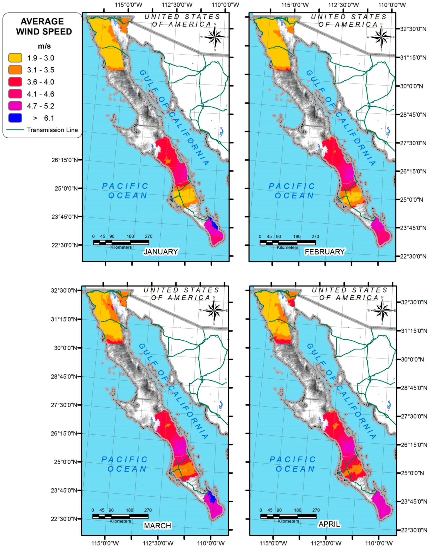
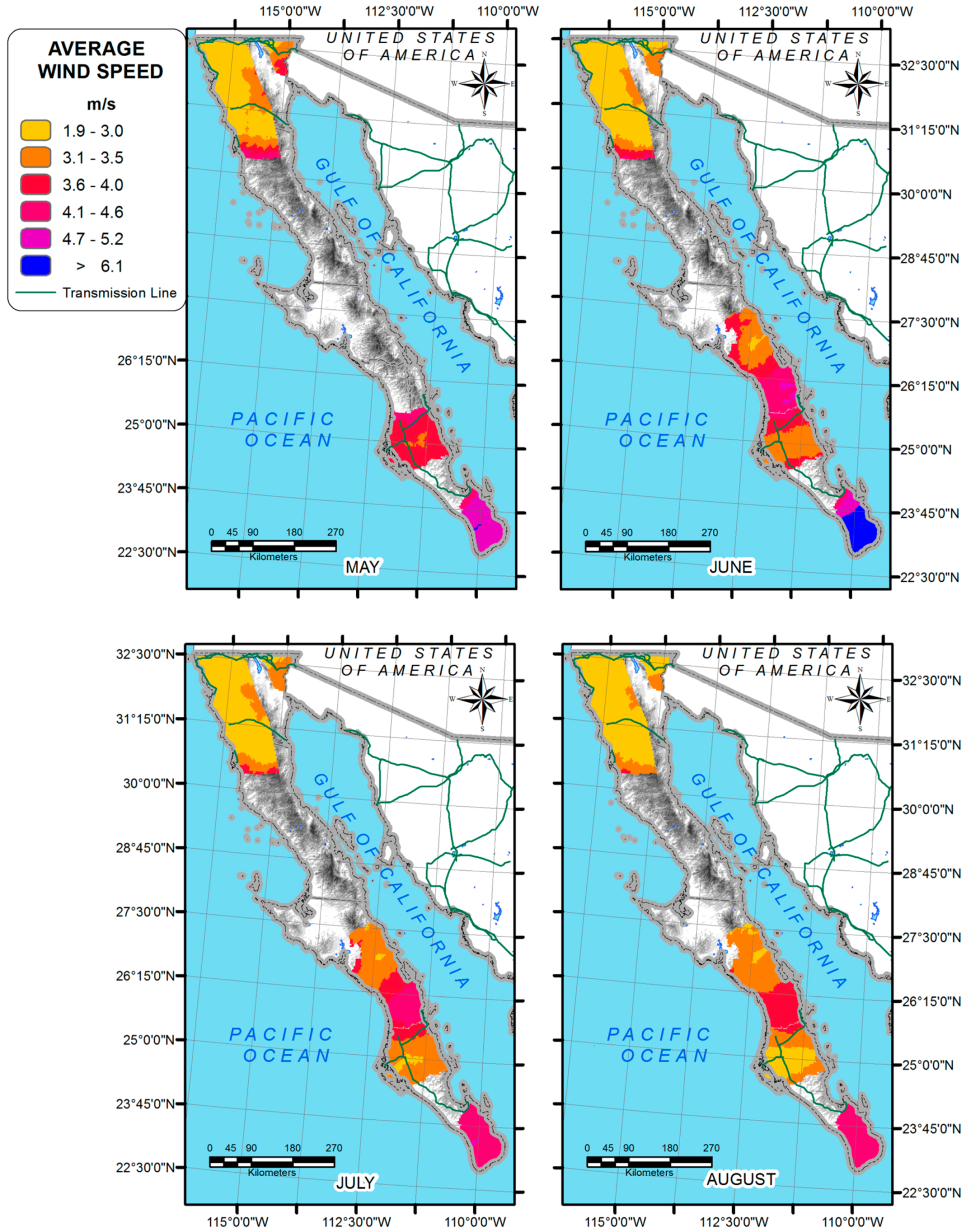
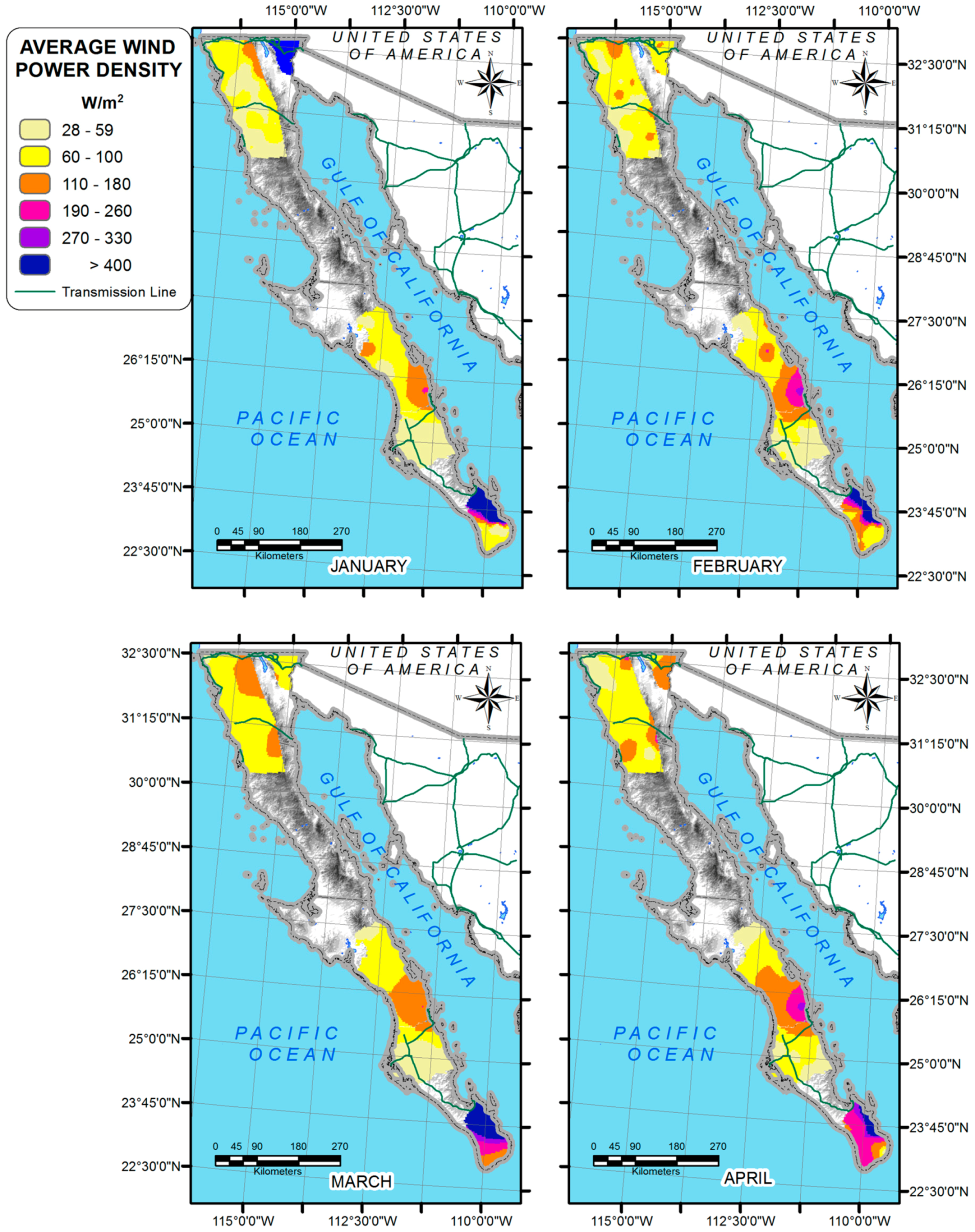
3.4. Wind Speed and WPD Maps

Maps consider data from AMSs, SAMSs and 80 points from SMSE to represent Kriging interpolation, these 80 points are along the peninsula to avoid interpolation problems. As a result of this interpolation, the maps will show zones with higher wind resource, the interpolation includes only small urban areas at the Peninsula, the rest of the territory has complex terrain which not include small urban zones, see Figure 8, Figure 9, Figure 10, Figure 11, Figure 12, Figure 13, Figure 14 and Figure 15.

The wind resource is well distributed along the Peninsula, however the zones with most wind power are located in the middle and south of it. It can be observed that the seasonal wind distribution, i.e., January, February (Figure 8) and September (Figure 10) are the months with the lowest wind resource in respect to other months. Figure 11 shows annual resources and it can be seen that the north is the zone with fewer wind resources, with values from 1.9 to 3 m/s, but can be used for stand-alone wind turbine or water pumps. WPD is shown in Figure 12, Figure 13, Figure 14 and Figure 15.

The WPD shows the power per square area in Cabo San Lucas (south) where almost the entire year has potential see Figure 12, Figure 13 and Figure 14. The annual WPD represented in Figure 15, shows that the area in the middle of the Peninsula is another zone with good potential, both areas having above 400 W/m². There are few zones with low potential, these areas having 28 to 59 W/m².

The small urban communities with good wind potential represent around 10%, most of which are in Baja California Sur and are located along its length; however, communities at Baja California with high wind resource are located to the north, the other communities with lower wind potential could use wind power for small wind mills or water pumps.

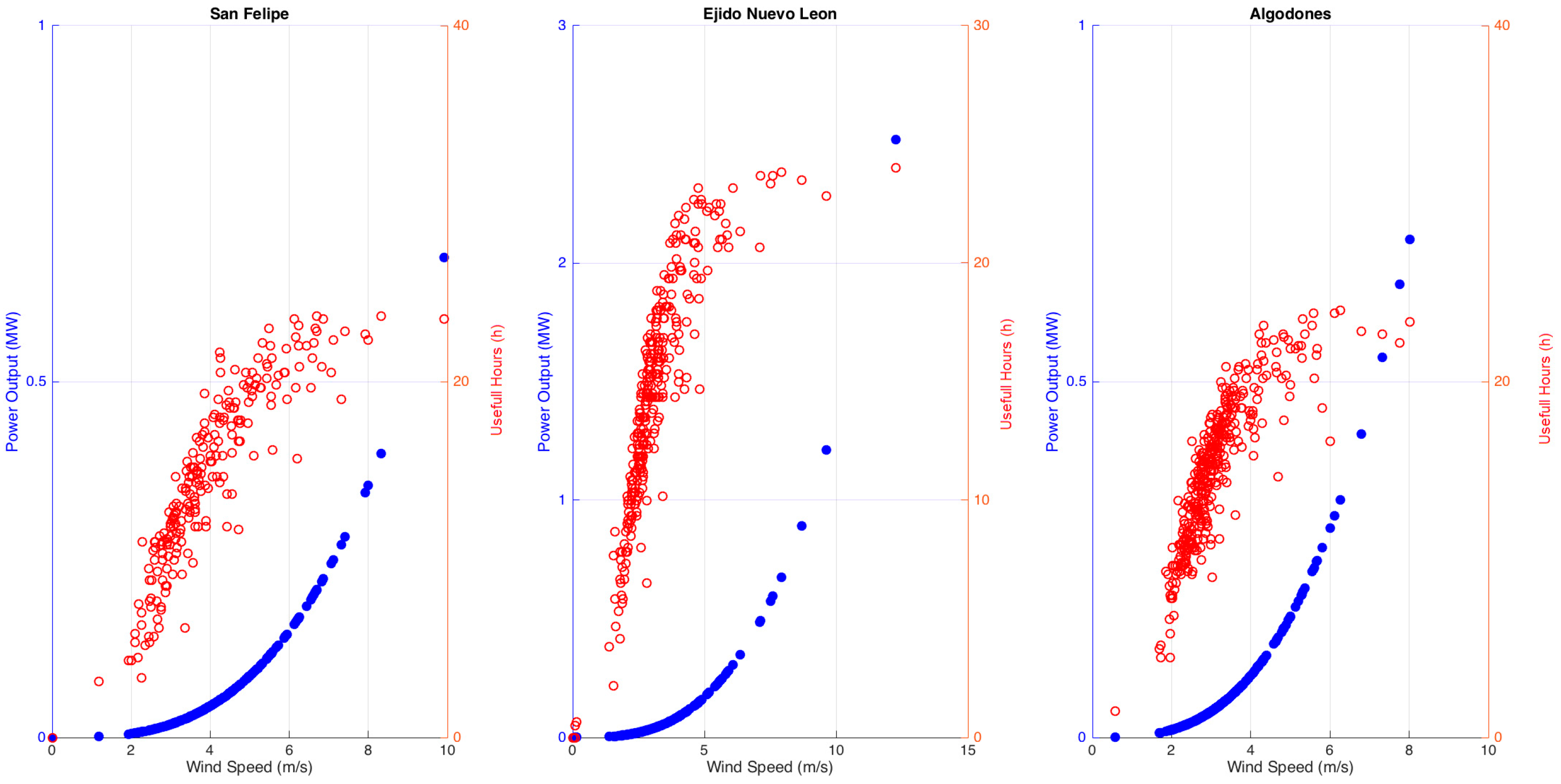
3.5. Wind Speed, Power Output Generated and Useful Hours

The relationship between wind speed, power output and useful hours gives accurate information of wind as a resource and it is necessary to show this relation in Figure 16, Figure 17, Figure 18 and Figure 19.

There are two important variables made when assessing wind speed: how much power is generated and the amount of useful hours for wind turbine. In Figure 16 it can be observed that Bahia Angeles has more than 2.5 MW and its useful hours are between 10 h and 24 h per day, Playas Rosarito and Tecate also have good wind characteristics, more than 1 MW and 15 useful hours.

In Figure 17, stations analyzed in Baja California Sur show that the amount of power is pleasing, Cabo San Lucas has more than 3.5 MW, Todos Santos, Bahia Loreto and Cabo Pulmon more than 2.5 MW each with 24 useful hours per day; only Gustavo Diaz Ordaz does not have good power generation because its power is less than 0.25 MW and its useful hours do not represent more than 1600 h/year (see Table 3) or 11 h per day.

In Figure 18, SAMSs at Baja California show good potential, Ejido Nuevo Leon has around 2.5 MW and 5290 h per year (see Table 3). SAMSs at Baja California Sur, Figure 19, shows that La Paz has almost 3 MW at 12 m/s and 5584 h per year (see Table 3) and Santa Rosal at 9 m/s can generate 1.2 MW and has 5674 h per year (see Table 3).

4. Discussion

The study illustrates the results of energy generation in the Baja California Peninsula, Mexico. The energy produced in small urban communities can contribute to the currently installed capacity in the country and in the renewable target plan for 2024.

At the Baja California Peninsula almost 5.13% of small urban communities are not electrified [21] with around 2500 small urban communities. The results of this study of wind power assessed in whole Peninsula would export 4407.6 kW or 38,603,666 kWh per year to the grid. Another necessary variable within wind assessment is the number of useful hours for the whole peninsula, with the mean at around 5220 h/year.

If analyzed separately, the peninsula on one side of Baja California presents results for the Weibull distribution of an AMS and a SAMS over 2 in its shape parameter, La Rumorosa and San Felipe respectively. The total net power and energy outputs are 1903.2 kW and 16,672,682 kWh per year respectively and the mean of useful hours is 5163.7 h/year. Meanwhile, Baja California Sur has higher wind resources, its total net power output is 2503.5 kW and the total net energy output is 21,930,984 kWh per year; respecting useful hours, it has 5370.8 h/year as mean which represents the south of the peninsula as having higher resources, however is important to mention that the most of the population is concentrated to the north.

WPD maps show good power resources per square meter and shows the areas with the highest wind power the area would correlate with the small urban zones as its user, i.e., the Baja California wind power can generate electric energy for around 12% of the communities, meanwhile in Baja California Sur the electric power generation could electrify almost 25% of small urban communities.

Finding the highest electric consumption by zone or by city could, by trying to determine the wind periodicity and wind direction for each location, create electricity for small urban communities could be researched in the future.

5. Conclusions

Electricity in Mexico has been a problem and where developing countries have 100% of urban zones electrified Mexico itself has only 98.7%, requiring major effort in achieving a higher percentage. The new energy reforms have opened the market to private investors, however some assessments must done across whole country. It is shown in this paper that wind at the Baja California Peninsula has a higher potential to participate in transmission, distribution and supply of electric energy to small urban zones. The north and the south of the Peninsula has the highest intensity of wind as well as WPD and it is in this zones that there the highest concentration of urban population. It would be interesting to research further in order to demonstrate higher consumption of electricity vs. the renewable energy extraction at the same time.

Fitting time series using an algorithm is a useful tool to fill gaps, it could be used to forecast meteorological variables such as wind speed, this algorithm draws graphs in order to determine data trends and choose the best option to data fit.

This work is an analysis of wind characteristics of Baja California Peninsula; as not enough wind sensors were installed in Mexico, satellite wind data was used in order to prove the relation between an R-square, Bias, SD and RMSE analysis, the results of which determined advantages to regions without enough wind sensors.

References

1. Secretaría de Energía (SENER). Available online: http://www.sener.gob.mx (accessed on 2 January 2016).
2. The World Bank. Available online: http://www.data.worldbank.org/indicator/SI.POV.RUHC (accessed on 3 January 2016).
3. International Energy Association (IEA). Available online: http://www.iea.org/statistics/statisticssearch/report/?country=Mexico&product=electricityandheat (accessed on 10 January 2016).
4. Secretaría de Energía (SENER). Balance de Energía 2014. Available online: http://www.gob.mx/cms/uploads/attachment/file/44353/Balance_Nacional_de_Energ_a_2014.pdf (accessed on 10 January 2016).
5. Analysis of Mexico’s New Electricity Industry Law. 2014. Available online: https://m.mayerbrown.com/Files/Publication/15cb6f04-748b-4836-a607-26c65997c1c1/Presentation/PublicationAttachment/0f38ad29-4abf-442b-aef9-319d68469310/UPDATE-AnalysisElectricityLaw_0814.pdf (accessed on 1 March 2016).
6. Ley de Transicion Energetica, Mexico. Available online: http://www.dof.gob.mx (accessed on 24 May 2016).
7. International Energy Association. IEA Wind Task 26. The Past and Future Cost of Wind Energy. Available online: https://www.ieawind.org/index_page_postings/WP2_task26.pdf (accessed on 14 January 2016).
8. Gutierrez-Vera, J. Use of renewable sources of energy in Mexico case: San Antonio Agua Bendita. IEEE Trans. Energy Convers. 1994. [Google Scholar] [CrossRef]
9. Huacuz, J.; Agredano, J. Beyond the grid: Photovoltaic electrification in rural Mexico. Progress Photovolt. 1998, 6, 379–395. [Google Scholar] [CrossRef]
10. Federal Commission of Electricity. Available online: http://www.cfe.gob.mx/ConoceCFE/1_AcercadeCFE/Lists/Publicaciones/Attachments/61/ProgramaSENERV2.pdf (accessed on 16 January 2016).
11. Masera, O. Sustainable Fuelwood Use in Rural Mexico. Available online: http://www.apps.webofknowledge.com/UA_GeneralSearch_input.do?product=UA&search_mode=GeneralSearch&SID=4BtQy8KMrELICBqS1uL&preferencesSaved (accessed on 16 January 2016).
12. Comisión Nacional Para el Uso Eficiente de la Energía. Available online: http://www.conuee.gob.mx/ (accessed on 20 January 2016).
13. Hernández-Escobedo, Q.; Manzano-Agugliaro, F.; Zapata-Sierra, A. The wind power of Mexico. Renew. Sustain. Energy Rev. 2010, 14, 2830–2840. [Google Scholar] [CrossRef]
14. Sliz-Szkliniarz, B.; Vogt, J. GIS-based approach for the evaluation of wind energy potential: A case study for the Kujawsko-Pomorskie Voivodeship. Renew. Sustain. Energy Rev. 2011, 15, 1696–1707. [Google Scholar] [CrossRef]
15. Aydin, N.Y.; Kentel, E.; Duzgun, S. GIS-based environmental assessment of wind energy systems for spatial planning: A case study from Western Turkey. Renew. Sustain. Energy Rev. 2010, 14, 364–373. [Google Scholar] [CrossRef]
16. Hernández-Escobedo, Q.; Saldaña-Flores, R.; Rodríguez-García, E.R.; Manzano-Agugliaro, F. Wind energy resource in Northern Mexico. Renew. Sustain. Energy Rev. 2014, 32, 890–914. [Google Scholar] [CrossRef]
17. Ramachandra, T.V.; Shruthi, B.V. Wind energy potential mapping in Karnataka, India, using GIS. Energy Convers. Manag. 2005, 46, 1561–1578. [Google Scholar] [CrossRef]
18. Su, M.C.; Kao, N.H.; Huang, W.J. Potential assessment of establishing a renewable energy plant in a rural agricultural area. J. Air Waste Manag. Assoc. 2012, 62, 662–670. [Google Scholar] [CrossRef] [PubMed]
19. Agugliaro, F.M. Gasification of greenhouse residues for obtaning electrical energy in the south of Spain: Localization by GIS. Interciencia 2007, 32, 131–136. [Google Scholar]
20. Viana, H.; Cohen, W.B.; Lopes, D.; Aranha, J. Assessment of forest biomass for use as energy. GIS-based analysis of geographical availability and locations of wood fired power plants in Portugal. Appl. Energy 2010, 87, 2551–2560. [Google Scholar] [CrossRef]
21. Gil, M.V.; Blanco, D.; Carballo, M.T.; Calvo, L.F. Carbon stock estimates for forests in the Castilla y León region, Spain. A GIS based method for evaluating spatial distribution of residual biomass for bio-energy. Biomass Bioenergy 2011, 35, 243–252. [Google Scholar] [CrossRef]
22. Hiloidhari, M.; Baruah, D.C. Rice straw residue biomass potential for decentralized electricity generation: A GIS based study in Lakhimpur district of Assam, India. Energy Sustain. Dev. 2011, 15, 214–222. [Google Scholar] [CrossRef]
23. Zhang, F.; Johnson, D.M.; Sutherland, J.W. A GIS-based method for identifying the optimal location for a facility to convert forest biomass to biofuel. Biomass Bioenergy 2011, 35, 3951–3961. [Google Scholar] [CrossRef]
24. Ghilardi, A.; Guerrero, G.; Masera, O. A GIS-based methodology for highlighting fuel wood supply/demand imbalances at the local level: A case study for Central Mexico. Biomass Bioenergy 2009, 33, 957–972. [Google Scholar] [CrossRef]
25. Moreno, A.; Gilabert, M.A.; Martinez, B. Mapping daily global solar irradiation over Spain: A comparative study of selected approaches. Solar Energy 2011, 85, 2072–2084. [Google Scholar] [CrossRef]
26. Arnette, A.N.; Zobel, C.W. Spatial analysis of renewable energy potential in the greater southern Appalachian mountains. Renew. Energy 2011, 36, 2785–2798. [Google Scholar] [CrossRef]
27. Gastli, A.; Charabi, Y. Solar electricity prospects in Oman using GIS-based solar radiation maps. Renew. Sustain. Energy Rev. 2010, 14, 790–797. [Google Scholar] [CrossRef]
28. Liu, M.; Bárdossy, A.; Li, J.; Jiang, Y. GIS-based modelling of topography-induced solar radiation variability in complex terrain for data sparse region. Int. J. Geogr. Inf. Sci. 2012, 26, 1281–1308. [Google Scholar] [CrossRef]
29. Vance, E. Mexico sets climate targets. Nature 2012. [Google Scholar] [CrossRef] [PubMed]
30. Bravo, J.; Casals, X.; Pascua, I. GIS approach to the definition of capacity and generation ceilings of renewable energy technologies. Energy Policy 2007, 35, 4879–4892. [Google Scholar] [CrossRef]
31. Ramachandra, T.V.; Shruthi, B.V. Spatial mapping of renewable energy potential. Renew. Sustain. Energy Rev. 2007, 11, 1460–1480. [Google Scholar] [CrossRef]
32. Belmonte, S.; Nuñez, V.; Viramonte, J.G.; Franco, J. Potential renewable energy resources of the Lerma Valley, Salta, Argentina for its strategic territorial planning. Renew. Sustain. Energy Rev. 2009, 13, 1475–1484. [Google Scholar] [CrossRef]
33. Ho-Jin, Y.; Jae-Jin, K. Assessment of observation environment for surface wind in urban areas using a CDF model. Korean Meteorol. Soc. 2015, 25, 449–459. [Google Scholar]
34. Instituto Nacional de Estadística y Geografía. Available online: http://www.inegi.org.mx (accessed on 30 January 2016).
35. Polo, J.; Zarzalejo, L.F.; Cony, M.; Navarro, A.A.; Marchante, R.; Martin, L.; Romero, M. Solar radiation estimations over India using Meteosat satellite images. Sol. Energy 2011, 85, 2395–2406. [Google Scholar] [CrossRef]
36. Zelenka, A.; Perez, R.; Seals, R.; Renne, D. Effective accuracy of satellite-derived hourly irradiations. Theor. Appl. Climatol. 1999, 62, 199–207. [Google Scholar] [CrossRef]
37. Vignola, F.; Harlan, P.; Perez, R.; Kmiecik, M. Analysis of satellite derived beam and global solar radiation data. Sol. Energy 2007, 81, 768–772. [Google Scholar] [CrossRef]
38. Pedro, H.T.C.; Coimbra, C.F.M. Assessment of forecasting techniques for solar power production with no exogenous inputs. Sol. Energy 2012, 86, 2017–2028. [Google Scholar] [CrossRef]
39. National Meteorological Service (NMS). Available online: http://www.smn.cna.gob.mx/emas/ (accessed on 1 February 2016).
40. Surface and Meteorology Energy System (SMES). Available online: https://www.eosweb.larc.nasa.gov/sse/ (accessed on 1 February 2016).
41. Lange, M. On the uncertainty of wind power predictions—Analysis of the forecast accuracy and statistical distribution of errors. J. Sol. Energy Eng. 2005, 127, 177–184. [Google Scholar] [CrossRef]
42. Jaramillo, O.A.; Saldana, R.; Miranda, U. Wind power potential of Baja California Sur, Mexico. Renew. Energy 2004, 29, 2087–2100. [Google Scholar] [CrossRef]
43. Manwell, J.F.; McGowan, J.G.; Rogers, A.L. Wind Energy Explained, Theory, Design and Application, 1st ed.; Wiley: Chichester, UK, 2009. [Google Scholar]
44. Lun, I.; Lam, J. A study of weibull parameters using long term wind observations. Renew. Energy 2000, 20, 145–153. [Google Scholar] [CrossRef]
Figure 1. Gap filling algorithm.
Energies 09 00805 g001
Figure 2. Geographic position of AMSs and SAMSs on the Baja California Peninsula, Mexico.
Energies 09 00805 g002
Figure 3. Distribution of small urban communities on the Baja California Peninsula, Mexico.
Energies 09 00805 g003
Figure 4. Weibull function at AMSs at Baja California.
Energies 09 00805 g004
Figure 5. Weibull function at AMSs at Baja California Sur.
Energies 09 00805 g005
Figure 6. Weibull function at SAMSs at Baja California.
Energies 09 00805 g006
Figure 7. Weibull function at SAMSs at Baja California Sur.
Energies 09 00805 g007
Figure 8. Average wind speed from January to April.
Energies 09 00805 g008
Figure 9. Average wind speed from May to August.
Energies 09 00805 g009
Figure 10. Average wind speed from September to December.
Energies 09 00805 g010
Figure 11. Annual wind speed at the Baja California Peninsula.
Energies 09 00805 g011
Figure 12. Average WPD from January to April.
Energies 09 00805 g012
Figure 13. Average WPD from May to August.
Energies 09 00805 g013
Figure 14. Average WPD from September to December.
Energies 09 00805 g014
Figure 15. Annual WPD.
Energies 09 00805 g015
Figure 16. Power output, useful hours and wind speed by AMSs Baja California.
Energies 09 00805 g016
Figure 17. Power output, useful hours and wind speed by AMSs Baja California Sur.
Energies 09 00805 g017
Figure 18. Power output, useful hours and wind speed by SAMs Baja California.
Energies 09 00805 g018
Figure 19. Power output, useful hours and wind speed by SAMs Baja California Sur.
Energies 09 00805 g019