Bioenergy and Food Supply: A Spatial-Agent Dynamic Model of Agricultural Land Use for Jiangsu Province in China

Shu, Kesheng; Schneider, Uwe A.; Scheffran, Jürgen

doi:10.3390/en81112369

Open AccessArticle

Bioenergy and Food Supply: A Spatial-Agent Dynamic Model of Agricultural Land Use for Jiangsu Province in China

by

Kesheng Shu

^1,2,3,*,

Uwe A. Schneider

⁴

and

Jürgen Scheffran

³

¹

Institute of Geographic Sciences and Natural Resources Research, Chinese Academy of Sciences, Beijing 100101, China

²

University of Chinese Academy of Sciences, Beijing 100049, China

³

Research Group Climate Change and Security, Institute of Geography, Center for Earth System Research and Sustainability, University of Hamburg, Hamburg 20144, Germany

⁴

Research Unit Sustainability and Global Change, Center for Earth System Research and Sustainability, University of Hamburg, Hamburg 20144, Germany

^*

Author to whom correspondence should be addressed.

Energies 2015, 8(11), 13284-13307; https://doi.org/10.3390/en81112369

Submission received: 31 July 2015 / Revised: 23 October 2015 / Accepted: 10 November 2015 / Published: 24 November 2015

(This article belongs to the Special Issue Advances in Biomass for Energy Technology)

Download

Browse Figures

Versions Notes

Abstract

:

In this paper we develop an agent-based model to explore a feasible way of simultaneously providing sufficient food and bioenergy feedstocks in China. Concerns over the competition for agricultural land resources between food and bioenergy supply hinder the further development of bioenergy, especially in China, the country that needs to feed the world’s largest population. Prior research has suggested the introduction of energy crops and reviewed the resulting agricultural land use change in China. However, there is a lack of quantitative studies which estimate the value, contribution, and impact of bioenergy for specific conditions at the county level and provide adequate information to guide local practices. To fill this gap, we choose the Jiangsu Province in China as a case study, build up a spatial-agent dynamic model of agricultural land use, and perform a sensitivity analysis for important parameters. The simulation results show that straw from conventional crops generally dominates Jiangsu’s biomass supply with a contribution above 85%. The sensitivity analyses reveal severe consequences of bioenergy targets for local land use. For Jiangsu Province, reclaimed mudflats, an alternative to arable lands for energy crop plantation, help to secure the local biomass supply and to alleviate the land use conflict between food and biomass production.

Keywords:

bioenergy supply; agent-based model; land use; general algebraic modeling system (GAMS); China

Graphical Abstract

1. Introduction

Modern bioenergy has experienced a worldwide boost in the last decades in response to concerns over energy security and climate change [1,2,3]. For some developing countries, bioenergy may also help to revive their agricultural sectors and rural areas [4,5]. However, rising food prices have sparked a debate as to whether and to what extent bioenergy development would put food supply at risk [6,7,8,9]. To simultaneously satisfy the demand for bioenergy feedstock and food, especially in the context of a fast growing bioenergy industry, previous studies have suggested a variety of options. These include improved agricultural practices, plantation of dedicated energy crops, use of cellulosic biomass conversion technology, exploitation of marginal or degraded lands, and joint production of energy and animal feed [10,11,12,13,14,15]. For China, a country accommodating the world’s largest population, finding a feasible compromise between food and bioenergy production is of great importance. Earlier qualitative studies addressed the introduction of energy crops to China’s cropping system [16,17,18] and the reclamation of mudflats for energy crop plantations [19,20,21]. Insights from these studies were integrated by the administrative bodies in a series of official development plans [22,23,24]. On the global and country level, a cluster of pioneering quantitative work has been done to explore and mitigate the resource competition between food and bioenergy. Yamamoto et al. [25] used a global-land-use-and-energy (GLUE-11) model to evaluate the global bioenergy potential. Schneider and McCarl [26] developed the Agricultural Sector and Mitigation of Greenhouse Gas (ASMGHG) model to examine the potential of biofuel for reducing greenhouse gas (GHG) emissions in the U.S., considering both food crops and energy crops. Johansson and Azar [27] created the Land Use Change Energy and Agriculture (LUCEA) model to analyze the competition between agricultural and energy systems in the same country. Havlík et al. [28] and Kraxner et al. [29] applied the Global Biosphere Management (GLOBIOM) model to estimate land use impacts of bioenergy targets at a global scale.

While previous research has presented ideas of how to mitigate the conflict between bioenergy feedstock supply and food supply at aggregated scales, there is limited analysis of the value, contribution, and impact of bioenergy strategies for specific local conditions, i.e., at the county level. Results from global or national models, however, may not be adequate to guide local practices. This is especially true for China, which is rarely touched on in existing quantitative research. To fill this gap, this study develops a spatial-agent dynamic model of agricultural land use to simulate the annual land use patterns after the introduction of energy crops. By choosing Jiangsu Province in China as a case study, this model provides specific results to guide the regional development of bioenergy. Furthermore, by using sensitivity analysis, we evaluate the impact of alternative bioenergy targets on the local agricultural land use and measure the role of reclaimed mudflats in alleviating the land use conflict between biomass and food supply.

The paper is structured as follows: first, we provide background information on the study area relevant to the construction of our model. Next, we present the analytical framework and briefly explain the individual components. More detailed information can be found in the Appendix. Subsequently, we present the simulation results including optimal patterns of land use and bioenergy feedstock supply. Finally, we provide a concluding discussion.

2. The Bioenergy Development in Jiangsu Province

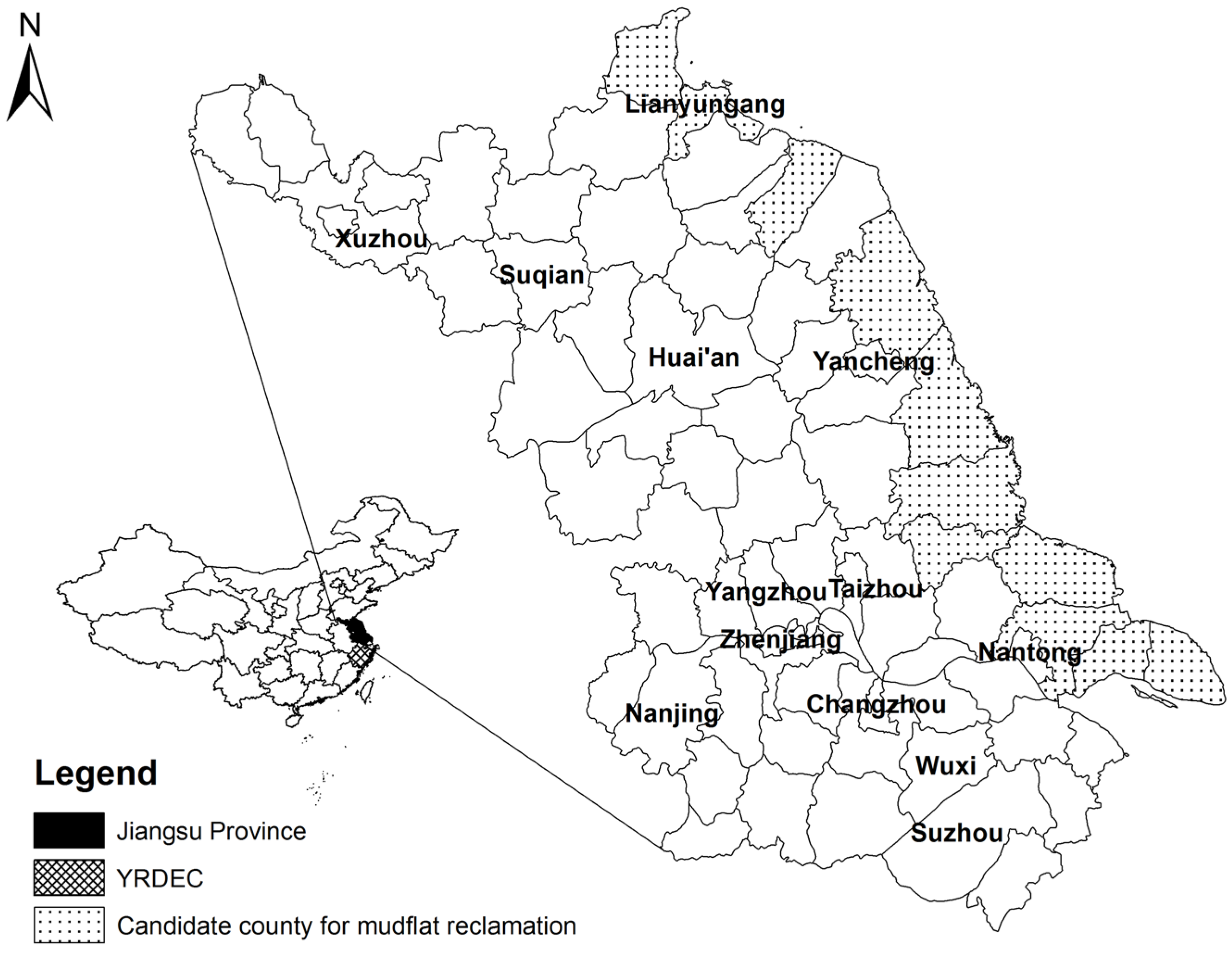
2.1. The Study Area

Jiangsu Province is located on the eastern coast of China. Together with Shanghai City and Zhejiang Province, it constitutes one of the most economically advanced areas of China, often referred to as the Yangtze River Delta Economic Circle (YRDEC). Jiangsu Province contains 13 prefecture-level cities, and each city administrates several county-level units with a total number of 102 (Figure 1). Due to differences in topography and socio-economic development, Jiangsu Province is often divided into three sub-regions: Southern Jiangsu, Central Jiangsu, and Northern Jiangsu.

Rapid economic growth in Jiangsu Province over the last 30 years has come at the expense of high GHG emissions. In 2007, the area’s estimated carbon emission totaled 144 million tonnes, with an annual growth rate of 14% during the period of 1996–2007 [30]. To curb CO₂ emissions, the provincial government issued an action plan, which includes the increasing use of renewable energy [31]. In 1990, up to 92% of Jiangsu’s carbon emissions came from the consumption of energy, with coal contributing the most [32]. Given that more than 92% of coal, 93% of crude oil and 99% of natural gas are imported from outside of Jiangsu [33], the use of domestic renewable energy sources, in particular, bioenergy can improve the region’s energy security. Besides reducing the use of fossil fuels, bioenergy can also stimulate rural development through bringing in investments in infrastructure and additional income opportunities for farmers. These benefits can help to reduce the migration flows from rural to urban areas and curtail the regional disparity within Jiangsu.

Figure 1. The location of Jiangsu Province. The list of potential counties for mudflat reclamation is identified in [23]. YRDEC is the acronym for the Yangtze River Delta Economic Circle.

While facing a high demand for bioenergy, Jiangsu Province also enjoys favorable local conditions for biomass production. The high output of grains implies a large amount of crop residues that could be used as a biomass feedstock. Furthermore, its particular location on the eastern coast enables access to additional land resources, i.e., reclaimed mudflats, which can be used for large-scale biomass production (Figure 2).

Figure 2. Supply and demand conditions for bioenergy development in Jiangsu Province.

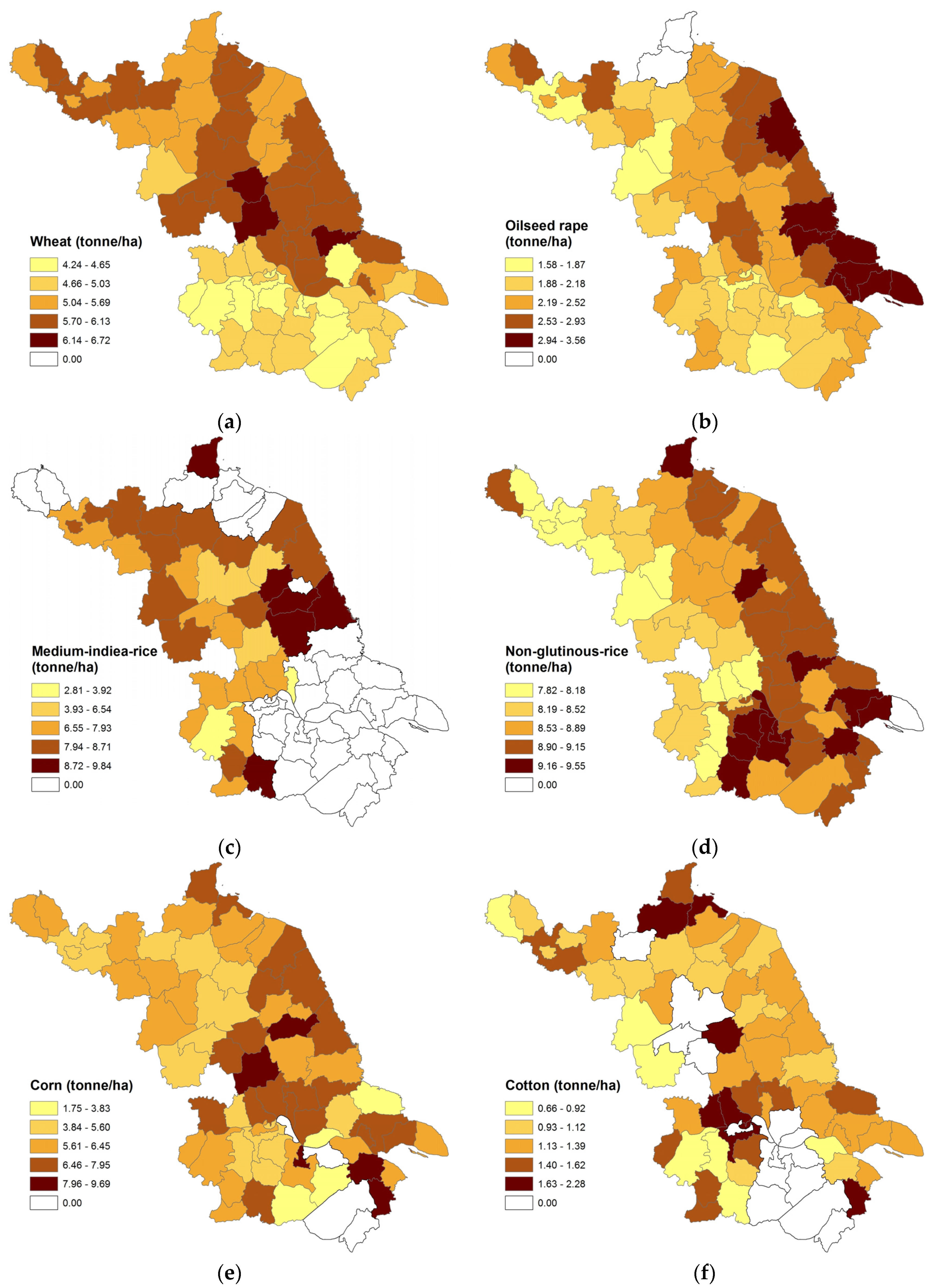
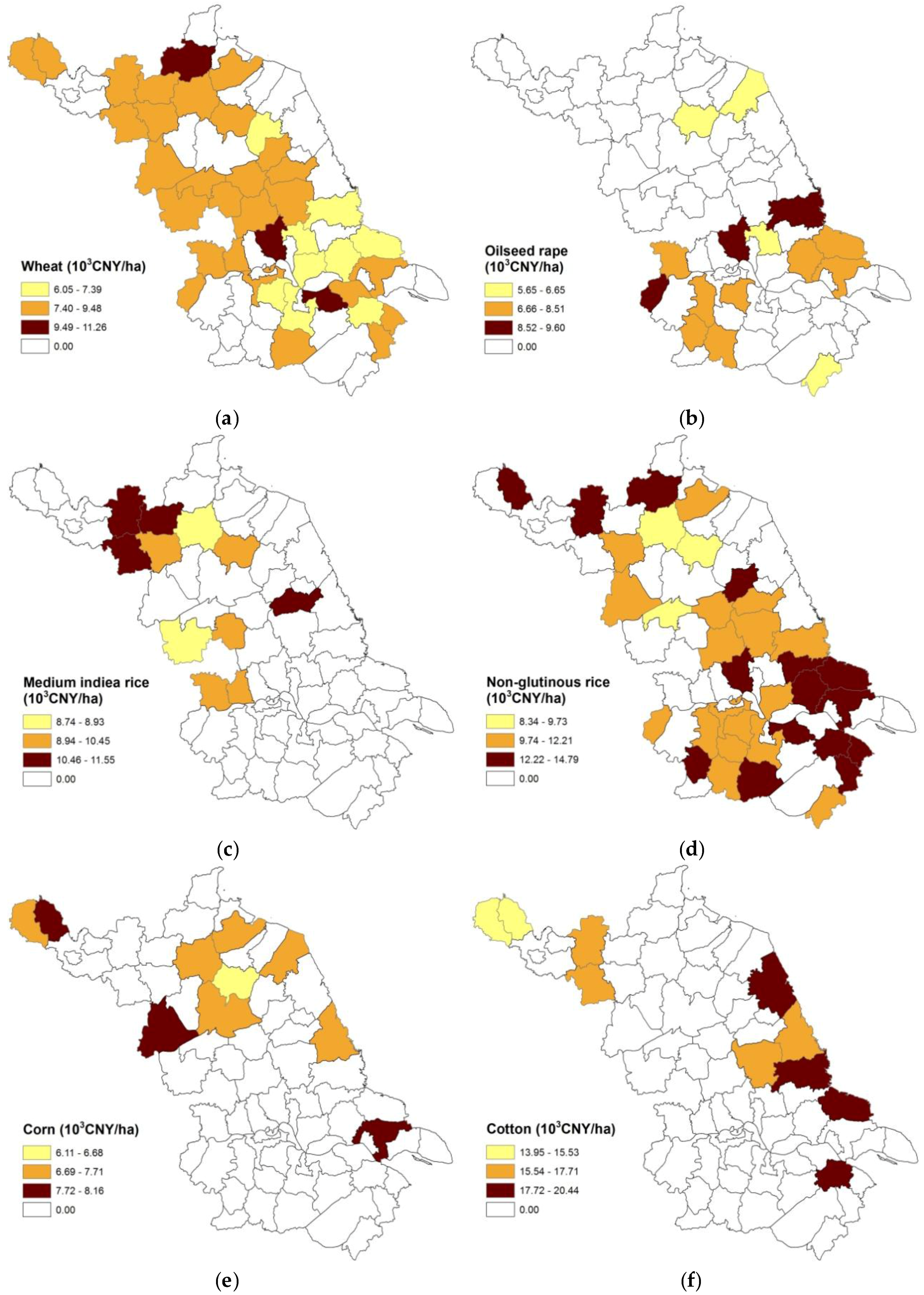
2.2. Conventional Crops

In order to distinguish dedicated energy crops, this study uses the term “conventional crops” for annual crops planted for the purpose of food, fodder, and industrial material production. In addition to grains or seeds, these crops offer straw as a source of bioenergy feedstock. However, we restrict the utilization ratio of this source to be less than 70% [34], due to the concerns over soil degradation and erosion caused by the excess removal of straw.

Figure 3. Crop yields in Jiangsu Province in 2010. (1) Data source: [35]; (2) The areas with yield data of 0.00 mean no plantation for that crop in practice. Data are presented for (a) wheat; (b) oil seed rape; (c) medium indiea rice; (d) non-glutinous rice; (e) corn; (f) cotton and (g) beans.

According to the official statistics [34], wheat, oilseed rape, medium indiea rice, non-glutinous rice, corn, cotton, and beans are the top cash crops in Jiangsu Province. Their respective planting areas account for more than 70% of Jiangsu’s total arable land. The straw from those crops contributes up to 88.5% of the provincial straw supply. Our model takes these seven plants as conventional crops and further categorizes them into summer crops and autumn crops, with respect to the local rotation cropping system. Figure 3 demonstrates the crop yields per hectare in 2010 on the county-level, with a five-scale color code representing five different levels of the yield. Cultivation cost data are obtained from the annual survey “Cost-Benefit Investigation of Jiangsu Agricultural Products” conducted by the Cost Investigation Supervision Branch of the Jiangsu Commodity Price Bureau. The available data span five years from 2006 to 2010 and were retrieved from answers to a questionnaire randomly distributed to the farmers across 57 representative counties belonging to 13 prefecture-level cities. Figure 4 illustrates the average costs for six main crops cultivated in Jiangsu Province in 2010. In the model, the per-hectare cost data which are reported in monetary values are converted to physical input requirements for specific production factors (including land, labour, fertilizer, pesticide and others), in accordance with the individual market price (or equivalent price).

Since the local cost-benefit survey does not include beans, historical county-level data are unavailable. To fill this gap, we employ the provincial-level data retrieved from the “Collection of Cost-Benefit Data of China’s Agricultural Products”. Similarly, for counties where certain crops are planted but cost-benefit data are not collected, we interpolate the data from neighboring areas by adopting the OrdinaryKriging Method offered in ArcGIS.

2.3. Energy Crops

In recent decades, a variety of lignocellulosic energy crops, including both perennial herbaceous crops (i.e., switchgrass, Miscanthus) and woody crops (such as willow, poplar, eucalyptus), have been introduced in many countries [36]. In China, however, large-scale commercialized plantation of energy crops is still absent. While we don’t have observed cultivation data for commercial energy crops, several research institutes have engaged in species selection and conducted small-scale field experiments in certain parts of China, including Jiangsu Province [16,37,38,39,40,41].

Figure 4. Crop cultivation cost in Jiangsu Province in 2010. (1) Data source: Data Collection of Cost-Benefit Investigation of Jiangsu Agricultural Products (2011); (2) Since the crop of beans is not covered by this Data Collection, county-level cost data are not available; (3) For areas showing a value of 0.00, data were not collected. Data are presented for (a) wheat; (b) oil seed rape; (c) medium indiea rice; (d) non-glutinous rice; (e) corn; (f) cotton.

In this study, we rely on the results of these experiments and discuss the selection from four candidate crops: switchgrass, silver reed, giant reed and miscanthus. Because these data are obtained from small-scale experiments under controlled conditions, they may not reflect all uncertainties of real agricultural operations and may not fully consider the potential environmental side effects.

Previous research reveals that the yield of energy crops reaches a plateau in the third year [42]. We adopt this finding and also define the total life span for each crop. In particular, switchgrass, silver reed and giant reed are set to live for 10 years, miscanthus for 20 years. After specifying the yield of each energy crop, we need to calculate its cultivation cost. First, we translate the experimental cost data of switchgrass, silver reed and giant reed measured from monetary values to physical input requirements for each production factor using individual factor prices. Second, we apply a reseeding rate of 25% to switchgrass and 0% to the other three crops [39,41]. Third, we extrapolate the cost data for switchgrass as a proxy for the unavailable cost data for miscanthus plantation. Particularly, we assume that the ratio of the cost of switchgrass to the cost of miscanthus is the same both in China and in the U.S. Then we apply this ratio obtained from the study in Illinois, USA [41] to the experimental data of switchgrass in China [40]. The resulting adaptive yields and cultivation costs of energy crops are shown in Table 1.

Table 1. Yield and cost data for potential energy crops in Jiangsu Province [16,37,38,39,40,41].

**Table 1.** Yield and cost data for potential energy crops in Jiangsu Province [16,37,38,39,40,41].
Items		Crops
		Switchgrass			Silver Reed			Giant Reed			Miscanthus
		Ages
		1	2	3–10	1	2	3–10	1	2	3–10	1	2	3–20
Yield (tonne/ha)		6.8	15.4	28.1	7	17.7	29	16.2	30.5	34.4	9.55	19.4	30.0
Cost (per ha)	Seedling (10³ CNY)	135	33.8	0	90	0	0	90	0	0	423.7	0	0
	Planting (d)	7.5	1.8	0	7.5	0	0	7.5	0	0	30.5	0	0
	Maintenance (d)	7.5	7.5	7.5	7.5	7.5	7.5	7.5	7.5	7.5	10.4	10.4	10.4
	Harvest (d)	15	15	15	15	15	15	15	15	15	44.7	44.7	44.7
	Irrigation (CNY)	600	0	0	600	0	0	600	0	0	600	0	0
	Water (CNY)	180	0	0	180	0	0	180	0	0	180	0	0
	Electricity (kWh)	846.8	0	0	846.8	0	0	846.8	0	0	846.8	0	0
	N-Fertilizer (kg)	150	150	150	150	150	150	150	150	150	165	69	103.5
	Herbicide (10³ kg)	3.8	0	0	3.8	0	0	3.8	0	0	4.1	0	0

2.4. Mudflats

The use of mudflats in Jiangsu Province as a potential land resource for energy crops has been thoroughly explored in many studies [43,44,45]. This option is considered by the local government in its “Outline of Reclamation and Utilization Plan for the Jiangsu Coastal Mudflats Resource (2010–2020)”. This guideline specified the concrete location, acreage, and utilization of reclaimed mudflats throughout three execution stages as shown in Table 2. Our model conforms to this guideline and assumes that reclaimed mudflats are exclusively used for energy crops. Thus, conventional crops can only be planted on arable lands, while energy crops can be planted either on arable lands or on reclaimed mudflats.

2.5. Biomass and Food Demand

In this study, we translate the objective of reconciling bioenergy feedstock provision and food supply into a set of mathematical restrictions. Particularly, the production of biomass and food is required to meet the respective demand levels. Therefore, the simulation results on land use patterns reflect the level of the two demands. The values of biomass demand in the years 2012 and 2015 are taken from [34], which considers four utilization options of biomass for energy purposes including biofuels, electric power, biochemicals, and solidification.

Table 2. The distribution of mudflats in Jiangsu Province and the extent of energy crop plantations in different periods (10³ ha) [22].

**Table 2.** The distribution of mudflats in Jiangsu Province and the extent of energy crop plantations in different periods (10³ ha) [22].
No.	Bank Section (Shoal)	County	Area Suitable for Reclamation
No.	Bank Section (Shoal)	County	Total	Period 1	Period 2	Period 3
A01	Xiuzhen estuary–Youwang estuary	Ganyu	1.00	0.00	0.47	0.00
A02	Xingzhuang estuary–Linhongkou	Ganyu	1.67	0.00	0.00	0.00
A03	Linhongkou–Xishu	Lianyungang	2.33	0.00	0.00	0.00
A04	Xuwei port	Lianyungang	4.67	0.00	0.00	0.00
A05	Xiaodong port–Xintan port	Xiangshui	1.33	0.60	0.00	0.67
A06	Shuangyang port–Yunliang estuary	Sheyang	1.00	0.00	0.00	0.93
A07	Yunliang estuary–Sheyang estuary	Sheyang	1.67	0.73	0.00	0.00
A08	Simaoyou estuary– Wanggang estuary	Dafeng	6.00	1.00	0.00	1.60
A09	Wanggang estuary–Chuandong port	Dafeng	5.00	2.53	0.00	2.20
A10-1	Chuandong port–Dongtai estuary	Dafeng	1.17	0.00	1.10	0.00
A10-2	Chuandong port–Dongtai estuary	Dongtai	1.17	0.00	1.10	0.00
A11	Tiaozini	Dongtai	26.67	8.00	9.33	0.00
A12-1	Fangtang estuary–Xinbeiling estuary	Dongtai	3.33	1.28	1.87	0.00
A12-2	Fangtang estuary–Xinbeiling estuary	Hai’an	2.00	1.92	0.00	0.00
A13	Xinbeiling estuary–Xiaoyangkou	Rudong	4.00	0.00	3.67	0.00
A14	Xiaoyangkou–Juejukou	Rudong	12.00	1.27	0.93	1.60
A15	Juejukou–Dongling port	Rudong	21.33	2.60	2.60	8.67
A16	Yaosha–Lengjiasa	Tongzhou	29.33	0.00	3.47	15.60
A17-1	Yaowang port–Haozhi port	Tongzhou	1.92	0.45	0.40	0.00
A17-2	Yaowang port–Haozhi port	Haimen	1.92	0.45	0.40	0.00
A17-3	Yaowang port–Haozhi port	Qidong	3.83	0.90	0.80	0.00
A18	Haozhi port–Tanglu port	Qidong	3.33	0.00	1.80	0.00
A19	Xiexing port–Yuantuojiao	Qidong	3.33	0.00	1.07	0.00
A20	Dongsha	Dongtai	21.33	0.00	0.00	13.87
A21	Gaoni	Dongtai	18.67	0.00	0.00	12.13
Total			180.00	21.73	29.01	57.27

Period 1: 2010–2012, Period 2: 2013–2015, Period 3: 2016–2020.

To curb the potential uncertainties of demand projections, we also collect other years’ data from the literature [46,47,48]. For intermediate years, the demand values are estimated through regression analysis. Food demand levels from 2011 to 2020 are based on previous study on Jiangsu’s food consumption [49]. The final demand data used in our study are listed in Table 3. To address the data uncertainty, we perform a sensitivity analysis.

Table 3. Demand targets for biomass and food demand between 2011 and 2030 (10³ t) [46,47,48,49].

**Table 3.** Demand targets for biomass and food demand between 2011 and 2030 (10³ t) [46,47,48,49].
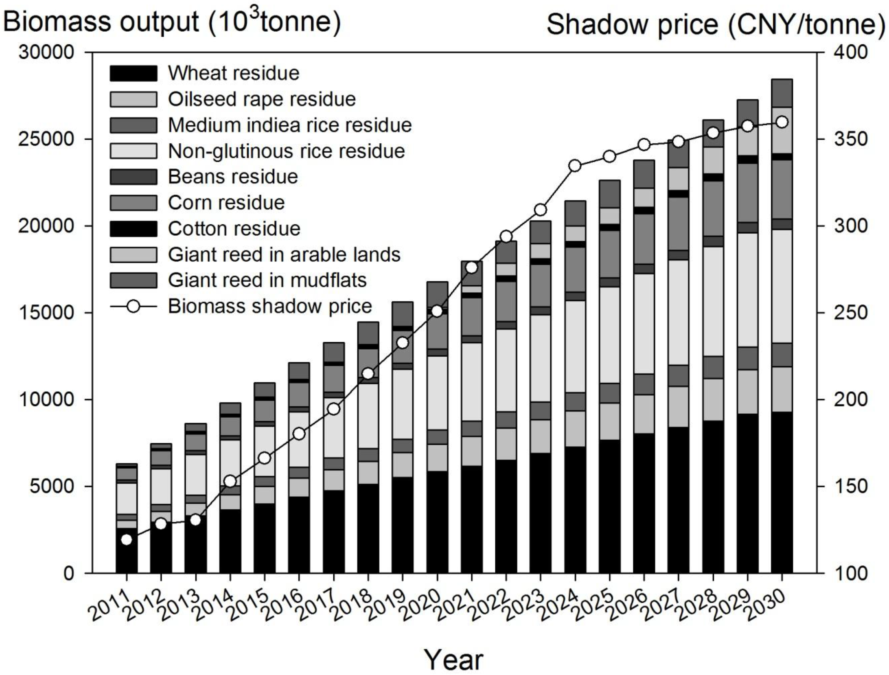
Year	2011	2012	2013	2014	2015	2016	2017	2018	2019	2020
Biomass	6302	7467	8632	9797	10,962	12,127	13,292	14,457	15,622	16,787
Food	29,720	29,885	30,050	30,214	30,379	30,544	30,708	30,873	31,038	31,203
Year	2021	2022	2023	2024	2025	2026	2027	2028	2029	2030
Biomass	17,952	19,117	20,282	21,447	22,612	23,777	24,942	26,107	27,272	28,437
Food	31,367	31,532	31,697	31,861	32,026	32,191	32,355	32,520	32,685	32,850

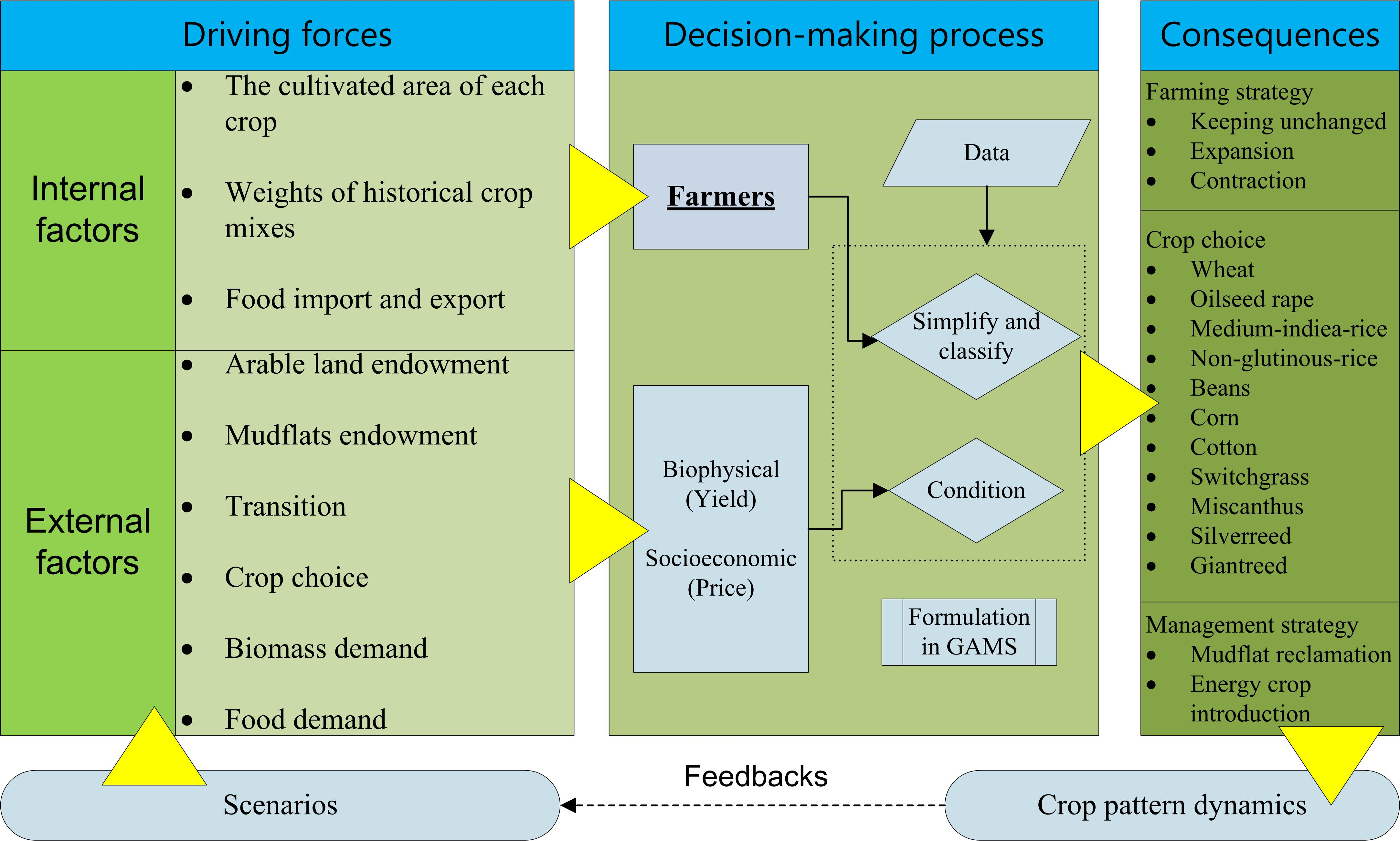
3. Model Design and Structure

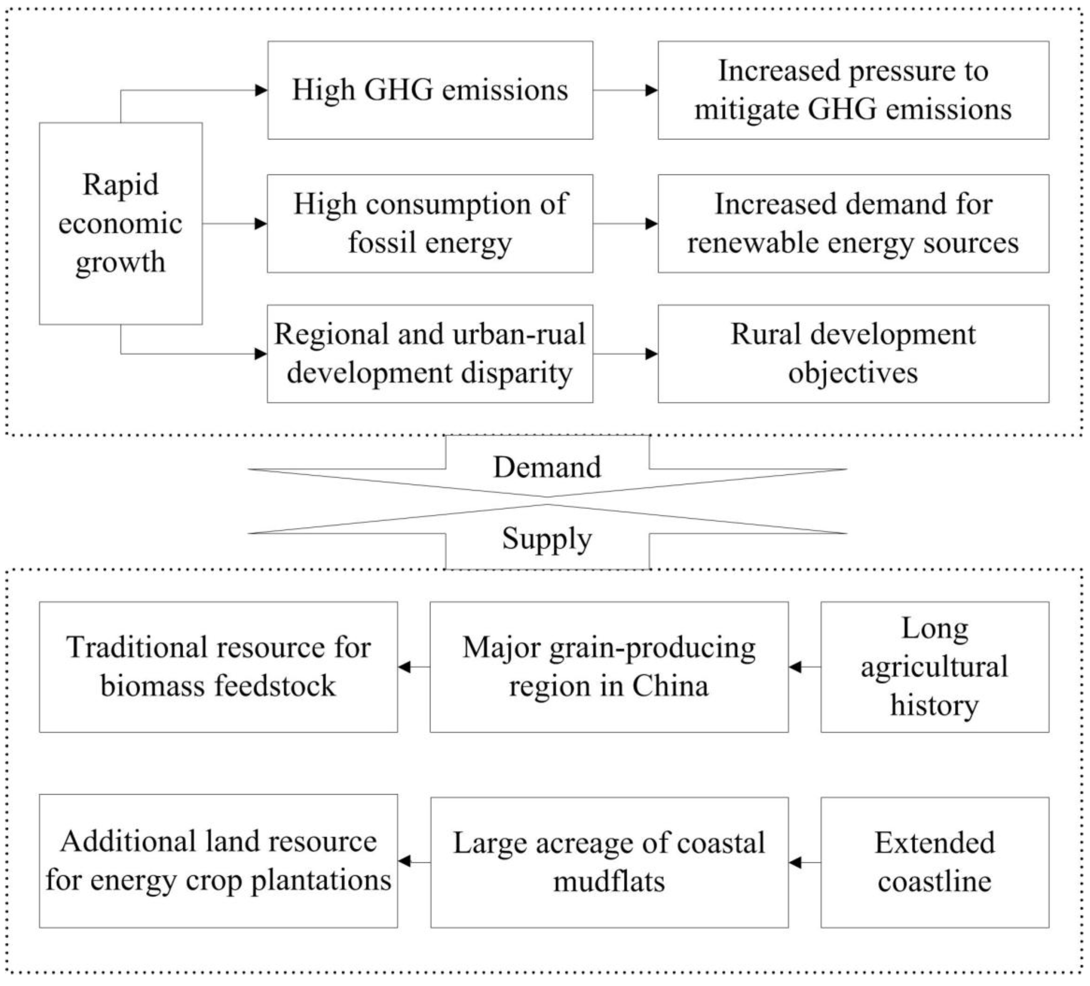
3.1. Model Framework

We develop a modelling framework to mimic the annually recurring decision-making process of farmers, i.e., the type and intensity of crops, which meets both food demand and biomass demand (Figure 5). The model framework integrates a spatial-agent system dynamic model and a partial equilibrium model of the agricultural sector. The former model was applied by Scheffran and BenDor in their simulation of the energy crop production in Illinois in the U.S. [1]. The advantage of this model is the maintained geographical characteristics of the individual farmers through using a spatial array of uniform grid cells to index their positions in the landscape. The model portrays the spatial relationships between farmers and depicts their particular geographical characteristics such as altitude, climate, shading, slope, and soil conditions. We aggregate Jiangsu’s 102 county-level administrative units into 70 counties by considering the administrative relations between neighboring units and the data accessibility. The conglomeration of all farmers in a county is considered as one agent in our regional agricultural sector model. This model component in our study was derived from the ASMGHG model developed by Schneider and McCarl [50], which links agricultural commodity markets to regionalized cropping systems. Similarly, our model couples the aggregation of each agent’s cropping system with the provincial bioenergy feedstock market.

Figure 5. The framework of the spatial-agent dynamic model of optimized agricultural land use.

The spatial-agent dynamic model of agricultural land use developed for this study combines the strength of both models: a) the depiction of heterogeneous geographical features of each agent leading to non-uniform opportunity costs for energy crops and b) Jiangsu’s bioenergy feedstock market, which determines the price of biomass through the intersection of aggregate supply from all farmers and governmental demand targets. Thus, a single farmer’s decision process is affected by the decisions of other farmers in the same market.

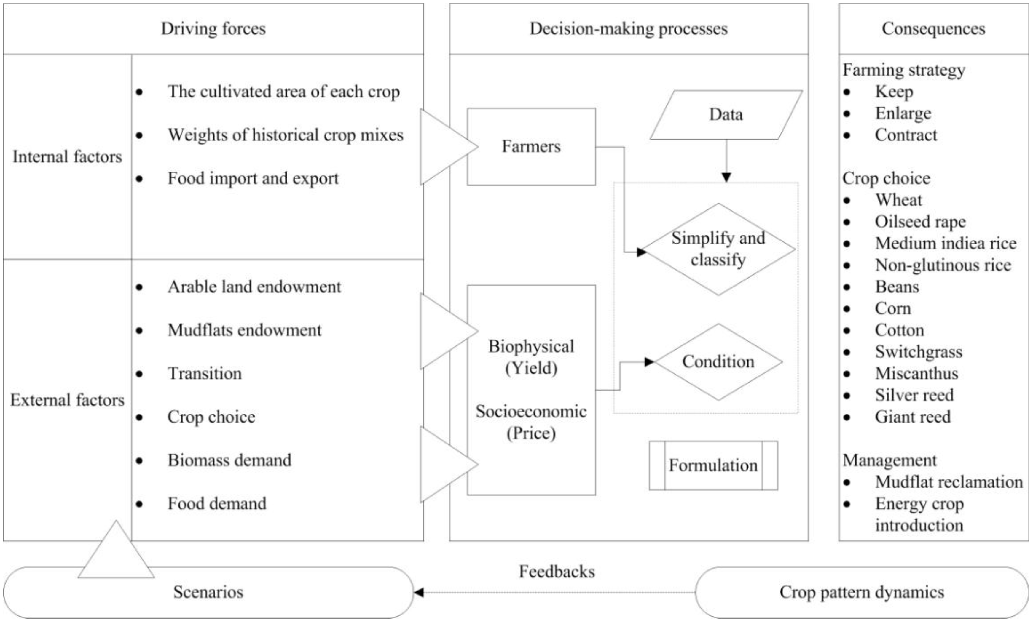
3.2. Model Structure

Our model determines the cost-efficient land use pattern, which simultaneously meets the demand for food and the demand bioenergy feedstock. This model is programmed in GAMS and consists of an objective function, a group of decision variables and a set of constraining equations. The objective function maximizes total agricultural economic surplus over a 20-year horizon with an annual time step. The values of the decision variables (internal factors in Figure 5) are endogenously determined through the optimization process. The constraining equations integrate environmental limits and market demands (external factors in Figure 5), which influences the farmers’ decision-making process. Mathematically, these equations define the convex feasible region for all decision variables. Each model element is briefly described in Table 4.

Table 4. The significance of model equations and variables.

**Table 4.** The significance of model equations and variables.
Model equation	Mathematical structure	Description
Objective function	$W E L F A R E = R E V E N U E - C O S T$	The sum of producer revenue in all commodity markets, minus specific and unspecific production cost and the cost of mudflat reclamation.
Resource limits	$L A N D^{concrop} + L A N D^{enecrop} \leq e n d o w m e n t^{arableland}$	The cultivated land in each region and time period cannot exceed given endowments.
	$L A N D^{mudflat} \leq e n d o w m e n t^{mudflat}$	According to Jiangsu’s official directive, a limited area of reclaimed mudflats mainly scattered in the coastal counties can be devoted to energy crop plantation.
	$\begin{array}{l} L A N D_{a, t}^{enecrop} \leq L A N D_{a - 1, t - 1}^{enecrop} \\ L A N D_{a, t}^{mudflat} \leq L A N D_{a - 1, t - 1}^{mudflat} \end{array}$	The area of energy crop plantation in higher age classes cannot exceed the area of the corresponding previous age class in the previous period.
	$\sum_{h i s} (l a n d u s e_{h i s}^{c o n c r o p} \times C M I X_{h i s}) = L A N D^{concrop}$	Cropping activities are restricted to a linear combination of historically observed choices. Onal and McCarl [51] find that historical crop mix restrictions implicitly embody numerous farming constraints, which are difficult to observe. These include crop rotation considerations, perceived risk reactions, and a variety of natural conditions.
	$\begin{array}{l} d e m a n d^{biomass} \leq y i e l d^{biomass} \times L A N D^{concrop} \\ + y i e l d^{biomass} \times (L A N D^{enecrop} + L A N D^{mudflat}) \end{array}$	Biomass production needs to satisfy minimum biomass demand.
	$\begin{array}{l} d e m a n d^{food} \leq y i e l d^{food} \times L A N D^{concrop} \\ + F O O D T R A D E \end{array}$	Food production needs to satisfy minimum food demand.
Decision variables	$L A N D^{concrop}, L A N D^{enecrop}, L A N D^{mudflat}$	Cultivated area includes arable lands and mudflats; Crops in the model are divided into conventional crops and energy crops.
	$C M I X$	The weights of historical land use patterns for decisions on land use in future years.
	$F O O D T R A D E$	Inter-provincial food trade.

Solving the model requires finding an optimal level for all decision variables subject to compliance with all constraining equations and, in the meantime, maximizing the objective function. As discussed by McCarl and Spreen [52], maximization of consumer and producer surplus yields the competitive market equilibrium. Thus, the optimal variable levels can be interpreted as likely equilibrium levels for agricultural activities under given economic, political and technological conditions. Simultaneously, the shadow prices, identical to the marginal values of the biomass and food demand constraint equations, determine market-clearing prices of food and bioenergy feedstock. A detailed description of our model is presented in the Appendix.

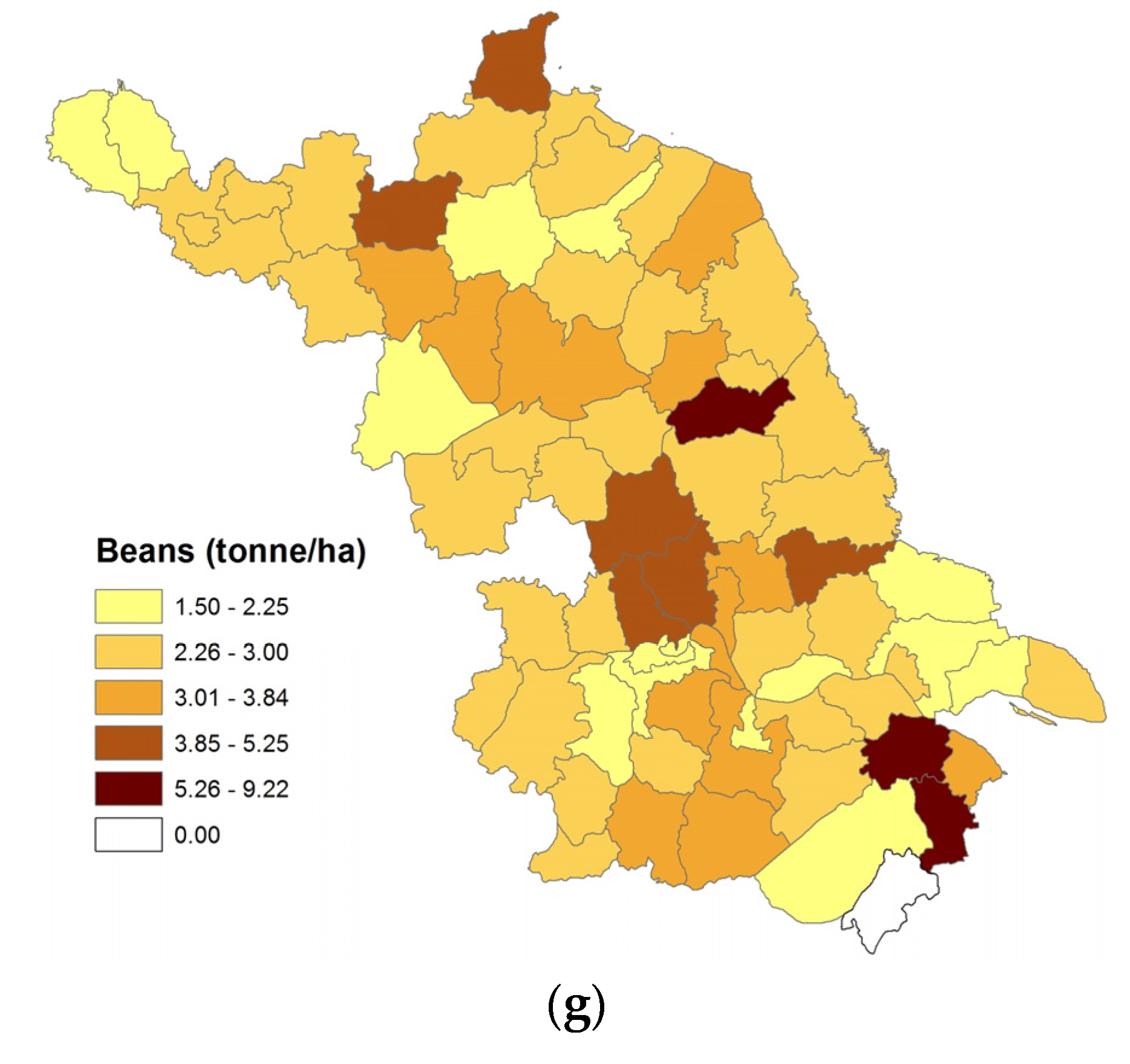
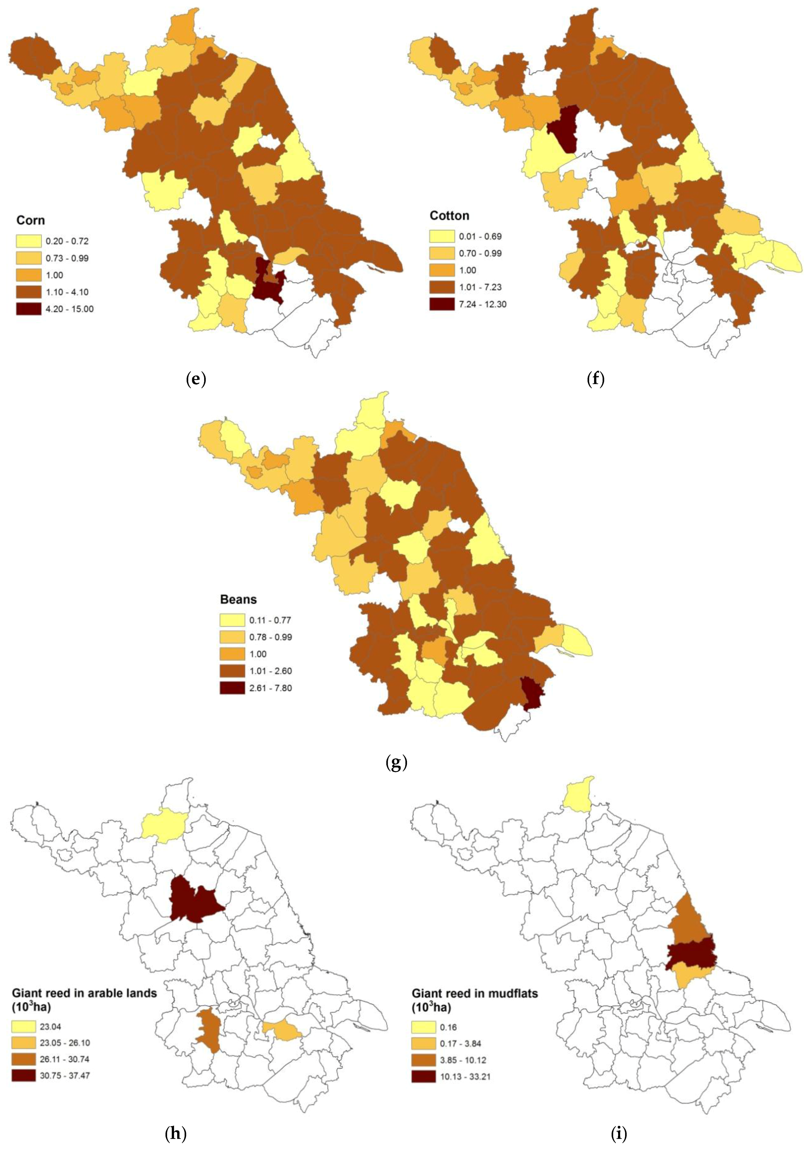
4. Simulation Results

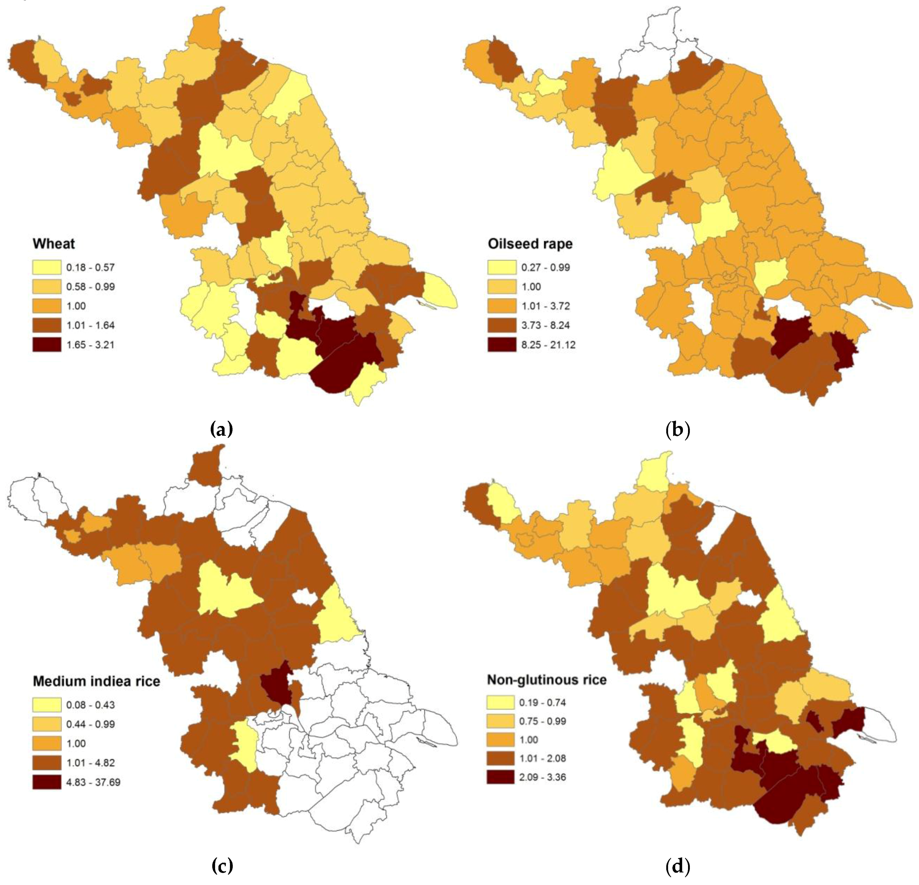
4.1. Land Use Patterns before and after the Introduction of Energy Crops

Starting from historically observed land use patterns in Jiangsu Province, the model results provide a cost-effective supply path of bioenergy feedstock for a steadily growing biomass demand. While the land use decisions are simulated for every year, we only show the cumulative change over the model’s entire time horizon.

Figure 6 shows the change in cultivated area between the initial and final year. Given that there is no commercial energy crop plantation in the base year, the land use changes for conventional crops and energy crops are presented in different ways: For conventional crops, relative land use changes are computed (Figure 6a–g), which are obtained by dividing the projected cultivated area for each crop in 2030 by the observed area in 2010. For energy crops, the absolute land use changes are shown, which are equal to the land areas in 2030 (Figure 6h,i). The land use change of conventional crops reveals two things: (1) The expansion of summer crops, i.e., wheat and oilseed rape, mainly occurs in Southern Jiangsu where oilseed rape expands extraordinarily fast (for example, its cultivated area has expanded 20 times in Wuxi City, 13 times in Kunshan County), thanks to its higher biomass output than wheat. (2) The land use changes for autumn crops differ across regions. Non-glutinous rice is mainly increased in Southern Jiangsu. By contrast, Northern Jiangsu favors more cotton, which is planted along the coastal line. Medium indiea rice is planted primarily in the eastern part of Jiangsu Province. For beans, on the other hand, they are found across the entire Jiangsu province.

Besides simulating the land use patterns for seven conventional crops, our model selects giant reed from four potential energy crops and suggests it to be planted on the arable lands in four out of 70 counties (namely in Jiangyin, Donghai, Huai’an and Jurong County) and on the reclaimed mudflats in four out of 10 counties (they are Hai’an, Ganyu, Dongtai and Dafeng County). In all counties where giant reed increases, conventional crops decrease and confirm the land use conflict between conventional and energy crops.

Figure 6. Projected land use change in Jiangsu Province in 2030 after the introduction of energy crops. Data are shown for (a) wheat; (b) oil seed rape; (c) medium indiea rice; (d) non-glutinous rice; (e) corn; (f) cotton and (g) beans; (h) giant reed planted in arable lands and (i) giant reed planted in mudflats. (1) Land use data for 2010 are retrieved from [35]; (2) White areas indicate zero plantations for particular crops.

4.2. Bioenergy Feedstock Supply

The simulation results disclose the sources of bioenergy feedstock supply (Figure 7). Straw from conventional crops constitutes the main source of bioenergy feedstock, contributing more than 85% of the total supply. The highest contribution comes from straw residues of two large-scale planted crops (wheat in summer and non-glutinous rice in autumn). Their relative shares remain similar throughout the twenty years of projection, reflecting a stable reproduction of the crop mix described in the item of crop choice in Table 4.

Figure 7. The projected bioenergy feedstock supply and its shadow price in Jiangsu Province for the period 2011–2030.

Up to 15% of the bioenergy supply comes from energy crops. Our results suggest giant reed first to be planted on reclaimed mudflats starting in 2011 and then extended to arable lands in 2020. Although giant reed starts on arable land at later phases, the contribution to biomass output is expected to surpass the contribution from mudflats in the year 2029. The area of giant reed on mudflats reaches a plateau at around 47 thousand ha with a production of 1.5 million tonnes of biomass in 2024 and afterwards.

Our model also determines the shadow price of bioenergy feedstock, i.e., the price society must pay to farmers in order to induce a sufficient amount of supply. To smooth out price fluctuations caused by the model’s dynamic structure, we use a simple 10-year moving average of each year’s shadow price. Figure 7 shows a steady increase of the biomass shadow price, which reflects the increase in the opportunity cost of biomass production induced by the rising bioenergy demand over time. As more biomass is demanded, less productive resources have to be gradually put into use and, therefore, lead to higher production cost. This upwards trend is sustained across the whole time horizon; however, in 2024 a turning point can be observed. A possible reason for this phenomenon is the use of the mudflats, whose reclamation cost outweighs other factors and thus dominates the total opportunity cost of biomass production. After 2024, there is no additional mudflat reclamation for the purpose of energy crop production. Thus, the expenditure on mudflat reclamation diminishes and reduces the rate of increase in opportunity cost.

4.3. Sensitivity Analysis 1: Bioenergy Feedstock Demand

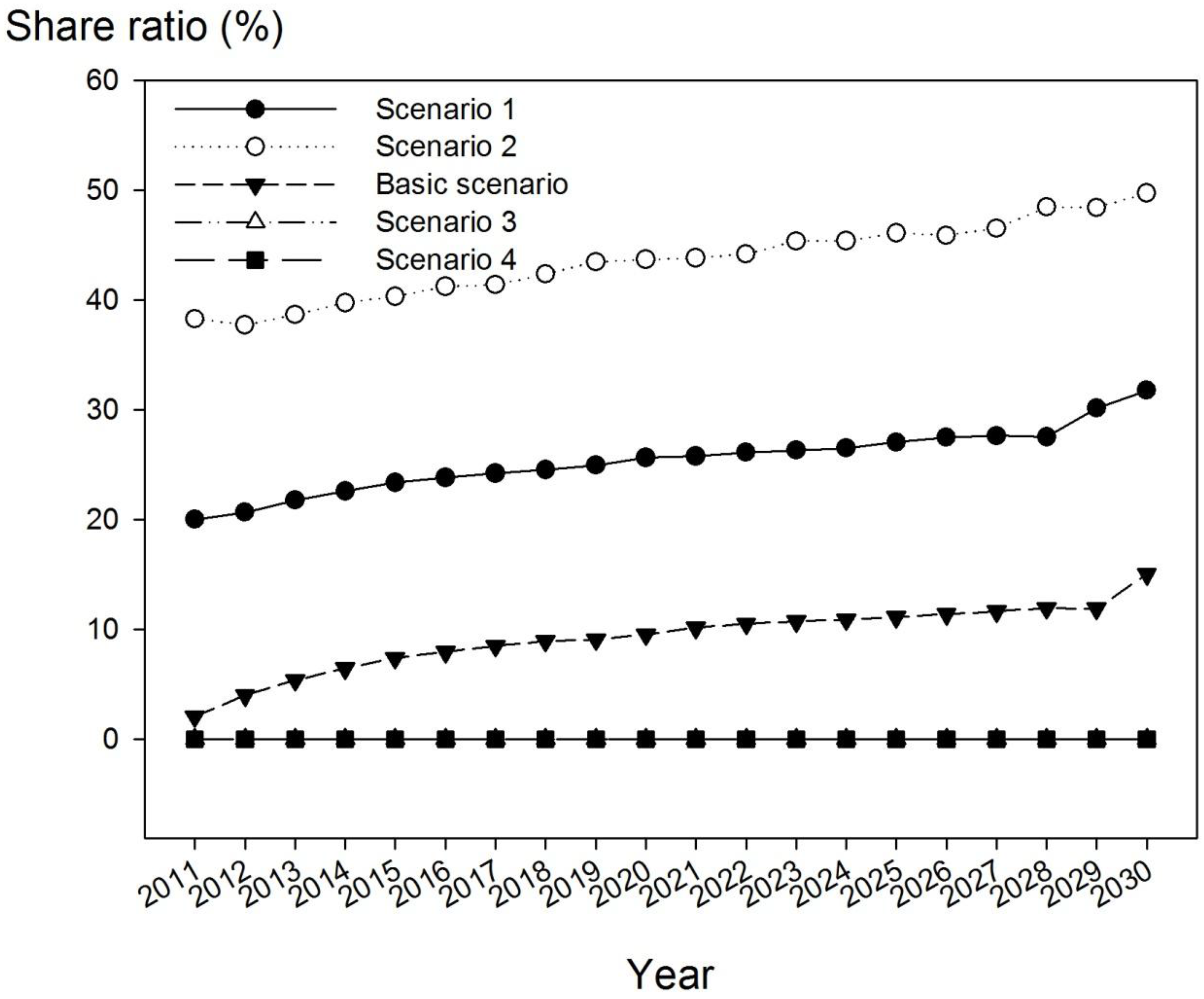
To find out how sensitive the optimal land use pattern is to the exogenously specified biomass demand targets, we analyze four alternative scenarios. These include two amplified demand scenarios (1.2 and 1.5 times as much as the biomass demand in the basic scenario) and two reduced demand scenarios (0.5 and 0.8 times as much as the biomass demand in the basic scenario).

4.3.1. The Introduction of Energy Crops

Our model computes optimal pathways for the introduction of energy crops in Jiangsu Province for a given biomass demand level. As shown in Figure 8, the curve representing the basic scenario suggests energy crops to be introduced early but with a small contribution. As biomass demand increases, the importance of energy crops jumps from 2% in 2011 to 15% in 2030, playing an auxiliary role in local biomass supply. For Jiangsu Province, this simulation result is a cost-effective way to simultaneously supply sufficient bioenergy feedstock and food by exploiting the dual-use of conventional crops (both food and energy use) and the single-use of energy crops (only energy use). A gradual and small-scale introduction of energy crops at the initial stage suggested by the model helps to realize a smooth transition process in the local agricultural sector towards the coordinated food and energy production, and to avert the potential resistance from local farmers who are used to traditional crop management practices.

Figure 8. The projected share of biomass from energy crops in bioenergy feedstock supply in Jiangsu Province between 2011 and 2030. Note: Under scenario 1 and 2 (the amplified demand scenarios), the biomass demands are set to 1.2 and 1.5 times the demand level in the basic scenario, respectively. In scenario 3 and 4 (the reduced demand scenarios), the respective demand multipliers are 0.5 and 0.8. Please note that the symbols representing scenario 3 and 4 always overlap each other.

However, we need to note that the above analysis is highly dependent on the given biomass demand level in the basic scenario. It is possible that different biomass demand levels may lead to differentiated land use patterns. As demonstrated in Figure 8, when the demand rises by 20% (scenario 1), the share of energy crops in biomass supply will ascend by more than 15%. If the demand climbs up for another 30% (scenario 2), the energy crops react by expanding their plantation and offering another 20% share. In this case, energy crops meet half of the total biomass demand in the final years. Instead, once the demand curtails by 20% or more (scenarios 3 and 4), energy crops will be completely ruled out from local biomass supply. These results conclude that in terms of the time and scale, the introduction of energy crops to Jiangsu Province is extremely sensitive to the level of biomass demand. The setting of bioenergy development targets would have far-reaching consequences, for example the timing of energy crop introduction, the plantation scale of energy crops and correspondingly, the distribution of other conventional crops.

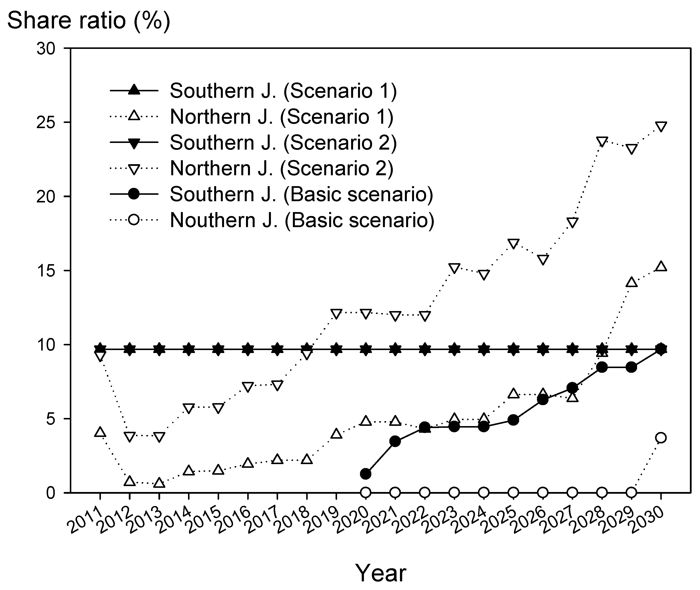
4.3.2. Differentiated Land Use Patterns in Jiangsu’s Three Sub-Regions

To echo the disparities in Jiangsu’s regional development, in this section we examine the introduction of energy crops on the level of the province’s three sub-regions, other than taking the whole province. Particularly, aiming at exploring the relationships between food and biomass supply, we only focus on the use of arable lands.

The allocations of arable lands between conventional crops and energy crops in three sub-regions perform quite different from each other: (1) Central Jiangsu always concentrates on the cultivation of conventional crops, no matter which level of biomass demand is applied. (2) The higher the biomass demand, the earlier and larger amounts of energy crops are to be planted on arable lands. As shown in Figure 9, energy crops are firstly introduced to the arable lands in the year of 2020 with the share of 2% in Southern Jiangsu under the basic scenario. By contrast, under the scenario 1, the crops firstly appear in 2011 with the share of 10% in Northern Jiangsu and 4% in Southern Jiangsu.

Figure 9. The projected share of energy crops on arable land in autumn in Jiangsu Province between 2011 and 2030. (1) Under scenarios 1 and 2 (the amplified demand scenarios), the biomass demands are set to 1.2 and 1.5 times as much as the demand level in the basic scenario, respectively; (2) As pointed out before, there are no energy crops in the reduced demand scenarios (scenarios 3 and 4), i.e., the share ratio of energy crops stays at 0. Thus, these scenarios are not shown in this figure; (3) Since there is no energy crop planted on arable lands in Central Jiangsu under all scenarios, this area is not included in the figure.

(3) The share of energy crops on the arable lands in Southern Jiangsu faces a distinct hurdle at around 10%. This finding implies that the arable land in Southern Jiangsu is the pioneer for energy crop plantation in the short term, though compared with Northern Jiangsu this area does not have enough potential to accommodate a large-scale plantation in the long term. This evidence corroborates the Jiangsu’s official orientation towards Northern Jiangsu as a bioenergy production basis, which was mentioned in the “Development Plan for the Coastal area of Jiangsu Province” in 2009.

4.4. Sensitivity Analysis 2: The Role of Mudflats

This section evaluates the role of mudflats in meeting the soaring biomass demand. We compare the basic scenario, where a certain fraction of mudflats is available for energy crops, with a situation in which all mudflats are excluded. Figure 10 uses three indicators to measure their role.

Figure 10. The role of mudflats measured in (a) biomass shadow price; (b) the share of energy crops on arable land; (c) food trade in Jiangsu Province between 2011 and 2030.

First, the presence of mudflats substantially lowers the shadow prices of bioenergy feedstock. For example, in the first ten years, the introduction of mudflats brings down the biomass price by more than 100 CNY/t (Figure 10a), which significantly decreases the purchasing cost of bioenergy feedstock and facilitates the development of bioenergy industry in Jiangsu Province, especially in the initial years. However, this effect diminishes along with the increasing biomass demand, because the share of energy crops on reclaimed mudflats in the biomass supply becomes small in the later years, especially after the year of 2024, the turning point of the use of reclaimed mudflats.

Second, the participation of mudflats alleviates the land use conflict between conventional crops and energy crops. In 2030, up to 2% of the arable land resources in the province could be saved and used for food production (Figure 10b).

Third, the mudflats help to produce an additional amount of about 0.75 million tonnes of food for cross-boundary food trade in 2030 (0.65 million tonnes more wheat and medium indiea rice for export, 0.10 million tonnes less beans and corn for import, as shown in Figure 10c), accounting for 3.59% of total amount of food trade in the same year.

Based on the results from the above analysis, it is safe to say that the accessibility to reclaimed mudflats can enhance the robustness of local biomass supply and relieve land use conflict between food and biomass production in Jiangsu Province, at the cost of mudflat losses.

5. Discussion and Conclusions

We develop a model to explore a cost-effective way to simultaneously reach food and bioenergy feedstock targets for Jiangsu Province. We apply this model to evaluate the impact of a bioenergy development plan on local agricultural land use and to measure the role of reclaimed mudflats in alleviating the land use conflict between bioenergy and food supply. The simulation results reveal the following insights: (1) The introduction of energy crops leads to seasonally differentiated land use patterns for conventional crops: the cultivation area of summer crops mainly expands in Northern Jiangsu. For autumn crops, such a pattern does not exist. (2) Energy crops are introduced first on arable lands in Jiangyin, Donghai, Huai’an and Jurong Counties and on reclaimed mudflats in the counties of Hai’an, Ganyu, Dongtai, and Dafeng. The economically preferred energy crop is giant reed. (3) The straws from conventional crops contribute more than 85% of the total biomass supply. Among these crops, wheat and non-glutinous rice top the bioenergy feedstock supply, followed by corn, oilseed rape, medium indiea rice, beans, and cotton. (4) On the provincial level, the introduction of energy crops is highly sensitive to the level of biomass demand. Therefore, alternative bioenergy development plans will result in different land use patterns. (5) On the sub-regional level, energy crops are employed first in Southern Jiangsu. However, over time, Northern Jiangsu cultivates energy crops on a larger area, supporting its status as a renewable energy production basis outlined in Jiangsu’s official development plan. (6) Reclaimed mudflats, as an alternative resource for energy crops, help secure the local biomass supply and alleviate the land use conflict between food and biomass production.

While the model offers useful insights into the bioenergy development in Jiangsu Province, two limitations should be noted: First, this research does not depict detailed biophysical characteristics of individual crop management systems. Thus, impacts on local biodiversity and ecosystem services are not considered. Second, this model suggests mudflats are an economically attractive resource for the cultivation of energy crops. While we consider possible environmental impacts of this resource and exclude ecologically sensitive areas, this study does not account for social side effects. For example, the model ignores the marginalization of smallholder farmers caused by the large-scale introduction of energy crops on reclaimed mudflats. Further research is needed to address the full spectrum of environmental and social side effects of bioenergy development.

Acknowledgments

This research was sponsored by the Chinese Scholarship Council (CSC) and the Austrian Federal Ministry of Science and Research (BMWF) through the Ernst Mach Grant, and in part by the German Science Foundation (DFG) through Hamburg University’s Cluster of Excellence "Integrated Climate System Analysis and Prediction". The authors thank involved governmental departments and bioenergy practitioners in Jiangsu Province for support in data collection.

Author Contributions

All authors together conceived and designed the model; Kesheng Shu performed the model, analyzed the data and wrote the paper with feedback by the co-authors.

Conflicts of Interest

The authors declare no conflict of interest.

Appendix

The Spatial-Agent Dynamic Model Specification

In the general formulation of the county-level dynamic agent-based model, the present value of the total profit is maximized across the whole time frame of a system covering the cultivation of both conventional crops and energy crops, subject to constraints on resource endowment, energy crop transition, cultivation selection and product demand.

Indices

u	county-level regions (Nanjing, Pukou, Liuhe, Shushui, Gaochun, Wuxi, Jiangyin, Yixing, Xuzhou, Fengxian, Peixian, Tongshan, Suining, Xinyi, Pizhou, Changzhou, Wujin, Liyang, Jintan, Suzhou, Changshu, Zhangjiagang, Kunshan, Wujiang, Taicang, Nantong, Tongzhou, Hai-an, Rudong, Qidong, Rugao, Haimen, Lianyungang, Ganyu, Donghai, Guanyun, Guannan, Huai-an, Lianshui, Hongze, Xuyi, Jinhu, Yancheng, Yandu, Xiangshui, Binhai, Funing, Sheyang, Jianhu, Dongtai, Dafeng, Yangzhou, Baoying, Yizheng, Gaoyou, Jiangdu, Zhenjiang, Dantu, Danyang, Yangzhong, Jurong, Taizhou, Xinghua, Jingjiang, Taixing, Jiangyan, Suqian, Shuyang, Siyang, Sihong)
fc	food crops (wheat, oilseed-rape, medium indiea rice, non-glutinous rice, beans, corn, cotton)
sc	summer crops (wheat, oilseed-rape)
ac	autumn crops (medium indiea rice, non-glutinous rice, beans, corn, cotton)
pc	perennial crops (switchgrass, miscanthus, silver reed, giant reed)
pr	products (wheat, seeds, medium indiea rice, non-glutinous rice, beans, corn, cotton, straw)
pr_food	non-bioenergy products (wheat, seeds, medium indiea rice, non-glutinous rice, beans, corn, cotton)
pr_energy	products as bioenergy feedstock (straw)
t	time horizon (2006–2020)
s	the current policy scenario (s1)
n	crop season (summer, autumn)
a	crop age (1,2,…,20)
ht	historical year (2000–2010)
inp	the input factors during crop field management (land, family labor, hired labour, water, n-fertilizer, p-fertilizer, k-fertilizer, o-fertilizer, pesticide, agricultural-film, diesel, electricity)

Exogenous Data

$y_{u, f c, p r, t, n}^{foodcrop}$	yield of food crop (tonne/ha)
$y_{p c, p r_e n e r g y, a}^{perennial crop}$	yield of perennial crop (tonne/ha)
$p s_{p r, t, s}$	price subsidy (CNY/tonne)
$v_{u, p r_f o o d, t}^{grains}$	price of non-biomass product (CNY/tonne)
$s u b_{u, f c, t, s}^{food crop}$	land subsidy for conventional crops (CNY/ha)
$s u b_{u, p c, t, s}^{perennial crop}$	land subsidy for perennial crops (CNY/ha)
$c^{mudflat}$	reclamation cost of mudflats (CNY/ha)
$b_{u, t}^{land}$	total arable land area (10³ ha)
$b_{u, t}^{mudflat}$	mudflats resource potential (10³ ha)
$h_{u, f c, h t, n}$	historical cultivation data (10³ ha)
$k_{p c}$	expected lifespan of perennial crops (year)
$d e m a_{t}^{b i o m a s s}$	demand of bioenergy feedstock (10³ tonne)
$d e m a_{t}^{g r a i n s}$	demand of grains (10³ tonne)
r	discount rate
$η_{u}$	proportion of straw for energy-end use (electricity and biofuels) to its total amount (%)
$α$	ratio of straw from main food crops (wheat, oilseed-rape, medium indiea rice, non-glutinous rice corn, cotton, beans) for its potential in the province (%)
$t e r m i n a l v a l u e_{u, p c, a}^{arableland}$	terminal value of perennial crop in arable land (CNY/ha)
$t e r m i n a l v a l u e_{u, p c, a}^{mudflat}$	terminal value of perennial crop in mudflats (CNY/ha)
$t e r m i n a l v a l u e_{u, f c, n}^{food crop}$	terminal value of food crop (CNY/ha)
$c o n s u m p t i o n_{f c, t, i n p, u}^{conventional crop}$	consumption of input factors for cultivation of conventional crops (ha/ha, d/ha, m³/ ha, kg/ha, kWh/ha)
$c o n s u m p t i o n_{p c, a, i n p}^{perennial crop}$	consumption of input factors for cultivation of perennial crops (ha/ha, d/ha, m³/ha, kg/ha, kWh/ha)
$v_{f c, t, i n p, u}^{cc input}$	price of input factors for food crops (CNY/ha, CNY/d, CNY/m³, CNY/kg, CNY/kWh)
$v_{t, i n p, u}^{pc input}$	price of input factors for perennial crops (CNY/ha, CNY/d, CNY/m³, CNY/kg, CNY/kWh)

Decision Variables

$L A N D_{u, f c, t, n}^{food crop}$	cultivated area for food crops in arable land (10³ ha)
$L A N D_{u, p c, t, a}^{perennial crop}$	cultivated area for perennial crops in arable land (10³ ha)
$L A N D_{u, p c, t, a}^{mudflat}$	cultivated area for perennial crops in reclaimed mudflats (10³ ha)
$C M I X_{u, t, h t, n}$	weights of historical data
$P R I C E_{t}^{biomass}$	endogenous price of biomass (CNY/tonne)
$F O O D F L O W_{f c, t}$	import or export amount of food trade (10³ t)

Objective Function

Max WELF =

\begin{array}{l} {\sum_{t} (1 + r)}^{- t} \cdot \\ (\begin{array}{l} \sum_{u, f c, p r_f o o d, n} [y_{u, f c, p r_f o o d, t, n}^{food crop} \cdot L A N D_{u, f c, t, n}^{food crop} \cdot (v_{p r_f o o d, t}^{grains} + p s_{p r_f o o d, t, s})] \\ + \sum_{u, f c, p r_e n e r g y, n} [y_{u, f c, p r_e n e r g y, t, n}^{food crop} \cdot L A N D_{u, f c, t, n}^{food crop} \cdot (P R I C E_{t}^{biomass} + p s_{p r_e n e r g y, t, s})] \\ + \sum_{u, f c, n} [L A N D_{u, f c, t, n}^{food crop} \cdot s u b_{u, f c, t, s}^{foodcrop}] \\ + \sum_{u, p c, p r_e n e r g y, a} [y_{p c, p r_e n e r g y, a}^{perennial crop} \cdot (L A N D_{u, p c, t, a}^{perennial crop} + L A N D_{u, p c, t, a}^{mudflat}) \cdot (P R I C E_{t}^{biomass} + p s_{p r_e n e r g y, t, s})] \\ + \sum_{u, p c, a} [(L A N D_{u, p c, t, a}^{perennial crop} + L A N D_{u, p c, t, a}^{mudflat}) \cdot s u b_{u, p c, t, s}^{perennial crop}] \end{array}) \\ + {(1 + r)}^{- t} \cdot \\ {\begin{cases} \sum_{u, p c, a} (L A N D_{u, p c, t, a}^{perennial crop} \cdot t e r m i n a l v a l u e_{u, p c, a}^{arable land} + L A N D_{u, p c, t, a}^{mudflat} \cdot t e r m i n a l v a l u e_{u, p c, a}^{mudflat}) |_{t =' 2030'} \\ + \sum_{u, f c, n} (L A N D_{u, f c, t, n}^{food crop} \cdot t e r m i n a l v a l u e_{u, f c, n}^{food crop}) |_{t =' 2030'} \end{cases}} \\ - {\sum_{t} (1 + r)}^{- t} \cdot \\ (\begin{array}{l} c^{mudflat} \cdot (\sum_{u, p c, a} L A N D_{u, p c, t, a}^{mudflat} - \sum_{u, p c, a} L A N D_{u, p c, t - 1, a}^{mudflat}) \\ + \sum_{u, f c, n} {\sum_{i n p} (c o n s u m p t i o n_{f c, t, i n p, u}^{conventional crop} \cdot v_{f c, t, i n p, u}^{cc input}) \cdot L A N D_{u, f c, t, n}^{food crop}} \\ + \sum_{u, p c, a} {\sum_{i n p} (c o n s u m p t i o n_{p c, a, i n p}^{perennial  crop} \cdot v_{t, i n p, u}^{pc input}) \cdot (L A N D_{u, p c, t, a}^{perennial crop} + L A N D_{u, p c, t, a}^{mudflat})} \end{array}) \\ \forall s \end{array}

(1)

The objective function Equation (1) of the model maximizes the present value of the net cash flows of the agriculture sector in Jiangsu Province across the whole time frame, as the total revenue minus costs. Specifically, the revenue of agriculture sector comprises of the sale of agricultural products, governmental agricultural subsidies and terminal values which are estimated for every crop. For energy crops, it is calculated as the Present Value of future profits of the rest of the productive life of the cultivation. This is equal to

P V = {\sum_{t} (P_{t} \cdot Y_{t} - P C_{t}) \cdot (1 + r)}^{- t}

, where

P_{t}

is the price of the crop’s product in period t,

Y_{t}

is the yield and

P C_{t}

is the production cost). The cost mainly covers land resource, labor resource, fertilizers, pesticides and other auxiliary inputs.

From line 1 to line 9, the revenue terms account for:

(1): The sales revenue of non-biomass from conventional crops;
(2): The sales revenue of biomass from conventional crops;
(3): The plantation subsidy on conventional crops;
(4): The sales revenue of biomass from energy crops;
(5): The plantation subsidy on energy crops;
(6): The terminal value of energy crops in the terminal year;
(7): The terminal value of conventional crops in the terminal year;

Starting from line 10 of the objective function, the cost items are:

(8): The reclamation cost of mudflats;
(9): The cost of production inputs for conventional crops;
(10): The cost of production inputs for energy crops.

Subject to

The most fundamental physical constraint on crop cultivation arises from the use of scarce and immobile resources. Particularly, the use of agricultural land is limited by given regional endowments of arable land and mudflat resources. In the following expressions,

b_{u, t}^{land}

denotes total arable land area in region u, year t and

b_{u, t}^{mudflat}

is total arable land area for the costal mudflat in region u and year t:

\sum_{f c} L A N D_{u, f c, t, n}^{food crop} + \sum_{p c, a} L A N D_{u, p c, t, a}^{perennial crop} \leq b_{u, t}^{lan d} \forall u, t, n

(2)

\sum_{p c, a} L A N D_{u, p c, t, a}^{mudflat} \leq \sum_{t =' 2006'}^{t} b_{u, t}^{mudflat} \forall u, t

(3)

Block in Equation (2) requires the sum of the arable lands allocated to certain types of crop plantation (including both conventional crops and energy crops) in one crop season to be smaller than the amount of locally accessible arable land resources, no matter which kind of field management has been adopted. This, to some extent, reflects the fact of land use conflict between food crops and energy crops. Similarly, for block in Equation (3), it applies the same structure as block in Equation (2). The difference is that block in Equation (3) proposes the limitation on mudflat resources and reclaimed mudflats are only dedicated to pc, which refers to the energy crop. As considering Jiangsu’s unique feature of having a large area of mudflats located along its coast, block in Equation (3) offers us a solution that the plantation of energy crop on mudflats may be a feasible and cost effective way to secure enough biomass provision for energy purposes while decreasing its negative influences on food security as much as possible:

\sum_{p c, a} L A N D_{u, p c, t - 1, a}^{mudflat} \leq \sum_{u, p c, t, a} L A N D_{u, p c, t, a}^{mudflat} \forall u, t

(4)

Block in Equation (4) assures that the reclamation process is irreversible. That means the accumulated cultivation area for energy crops in mudflats can only be enlarged. This assumption is consistent with an increasing tendency of biomass demand:

{\begin{array}{l} - L A N D_{u, p c, t - 1, a - 1}^{perennial crop} + L A N D_{u, p c, t, a}^{perennial crop} \leq 0 \\ - L A N D_{u, p c, t - 1, a - 1}^{mudflat} + L A N D_{u, p c, t, a}^{mudflat} \leq 0 \end{array} |}_{1 < a \leq k_{p c}} \forall u, p c, t, a

(5)

Block in Equation (5) is targeted for perennial crops’ consistency. Considering its natural death or farmers’ active eradication, the plantation area of certain kind of perennial crop would never be larger but only smaller than or be equal to the area of itself in the prior year.

The fifth set of constraints addresses aggregation related aspects of the farmers’ decision process. These constraints force farmers’ cropping activities for

L A N D_{u, f c, t, n}^{food crop}

either in summer or in autumn to fall within a convex combination of historically observed seasonal choices

h_{u, f c, h t, n}

(Equation (6)). Based on decomposition and economic duality theory, Onal and McCarl [53] show that historical crop mixes represent rational choices embodying numerous farm resource constraints, crop rotation considerations, perceived risk reactions, and a variety of natural conditions. In Equation (6), the

h_{u, f c, h t, n}

coefficient contains the observed crop mix levels for the latest 11 years (from 2000 to 2011).

C M I X_{u, t, h t, n}

, representing the weights of historical data in different years, are positive, endogenous variables indexed by historical year and region, whose level will be determined during the optimization process:

- \sum_{h t} (h_{u, f c, h t, n} \cdot C M I X_{u, t, h t, n}) + L A N D_{u, f c, t, n}^{food crop} = 0 |_{2010 < t \leq 2030} \forall u, f c, t, n

(6)

However, crop mix constraints are not applied to the crops, which under certain policy scenarios are expected to expand far beyond the upper bound of historical relative shares [54]. As the cultivation area of energy crops is expected to greatly expand in the future, these crops are naturally excluded from this equation block:

\begin{array}{l} d e m a_{t}^{biomass} - \sum_{u, f c, p r_e n e r g y, n} η_{u} \cdot \frac{y_{u, f c, p r_e n e r g y, t, n}^{food crop} \cdot L A N D_{u, f c, t, n}^{food crop}}{α} \\ - \sum_{u, p c, p r_e n e r g y, a} y_{u, p c, p r_e n e r g y, t, a}^{perennial crop} \cdot (L A N D_{u, p c, t, a}^{perennial crop} + L A N D_{u, p c, t, a}^{mudflat}) \leq 0 \forall t \end{array}

(7)

The supply and demand balance of biomass is represented in block in Equation (7). The first item denotes the biomass demand in a certain year. The second item denotes the biomass from traditional food crops, namely crop straw, and the last term represents the biomass from perennial crops grown either on arable land or reclaimed mudflats. This expression fully secures the achievement of biomass development targets in due year:

d e m a_{f c, t}^{grains} - \sum_{u, f c, p r_f o o d, n} (y_{u, f c, p r_f o o d, t, n}^{food crop} \cdot L A N D_{u, f c, t, n}^{food crop}) - F O O D F L O W_{f c, t} \leq 0 \forall f c, t

(8)

Paralleling, the last constraint set defines the satisfaction to the requirement of food security in the background of bioenergy introduction. The first item is the demand of certain food, the following items stand for the produced food from planted conventional crops, and the last item means the gap between food demand and supply is filled by cross-boundary food trade.

References

Scheffran, J.; BenDor, T. Bioenergy and land use: A spatial-agent dynamic model of energy crop production in Illinois. Int. J. Environ. Pollut. 2009, 39, 4–27. [Google Scholar] [CrossRef]
Hall, D.O.; House, J.I. Reducing atmospheric CO₂ using biomass energy and photobiology. Energy Convers. Manag. 1993, 34, 889–896. [Google Scholar] [CrossRef]
Jungmeier, G.; Spitzer, J. Greenhouse gas emissions of bioenergy from agriculture compared to fossil energy for heat and electricity supply. Nutr. Cycl. Agroecosyst. 2001, 60, 267–273. [Google Scholar] [CrossRef]
Demirbas, A.H.; Demirbas, I. Importance of rural bioenergy for developing countries. Energy Convers. Manag. 2007, 48, 2386–2398. [Google Scholar] [CrossRef]
Silveira, S. How to realize the bioenergy prospects? In Bioenergy—Realizing the Potential; Elsevier: Oxford, UK, 2005; pp. 3–17. [Google Scholar]
Ewing, M.; Msangi, S. Biofuels production in developing countries: Assessing tradeoffs in welfare and food security. Environ. Sci. Policy 2009, 12, 520–528. [Google Scholar] [CrossRef]
Tirado, M.C.; Cohen, M.J.; Aberman, N.; Meerman, J.; Thompson, B. Addressing the challenges of climate change and biofuel production for food and nutrition security. Food Res. Int. 2010, 43, 1729–1744. [Google Scholar] [CrossRef]
Scheffran, J. Biofuel conflicts and human security: Toward a sustainable bioenergy life cycle and infrastructure. Swords Ploughsh. 2009, 27, 4–10. [Google Scholar]
Ajanovic, A. Biofuels versus food production: Does biofuels production increase food prices? Energy 2011, 36, 2070–2076. [Google Scholar] [CrossRef]
Ugarte, D.D.L.T.; He, L. Is the expansion of biofuels at odds with the food security of developing countries? Biofuels Bioprod. Biorefining 2007, 1, 92–102. [Google Scholar] [CrossRef]
Campbell, J.E.; Lobell, D.B.; Genova, R.C.; Field, C.B. The global potential of bioenergy on abandoned agriculture lands. Environ. Sci. Technol. 2008, 42, 5791–5794. [Google Scholar] [CrossRef] [PubMed]
Scheffran, J. Criteria for a sustainable bioenergy infrastructure and lifecycle. In Plant Biotechnology for Sustainable Production of Energy and Co-Products; Mascia, P.N., Scheffran, J., Widholm, J.M., Eds.; Springer: Heidelberg, Germany, 2010; Volume 66, pp. 409–447. [Google Scholar]
Thomas, V.M.; Choi, D.G.; Luo, D.; Okwo, A.; Wang, J.H. Relation of biofuel to bioelectricity and agriculture: Food security, fuel security, and reducing greenhouse emissions. Chem. Eng. Res. Des. 2009, 87, 1140–1146. [Google Scholar] [CrossRef]
Ceotto, E.; Candilo, M.D. Sustainable bioenergy production, land and nitrogen use. Sustain. Agric. Rev. 2011, 5, 101–122. [Google Scholar]
Sadhukhan, J.; Ng, K.S.; Hernandez, E.M. Biorefineries and Chemical Processes: Design, Integration and Sustainability Analysis; John Wiley & Sons: Hoboken, NJ, USA, 2014. [Google Scholar]
Zong, J.; Guo, A.; Chen, J.; Liu, J. A study on biomass potentials of perennial gramineous energy plants. Pratac. Sci. 2012, 29, 809–813. [Google Scholar]
Shao, H.; Chu, L. Resource evaluation of typical energy plants and possible functional zone planning in China. Biomass Bioenergy 2008, 32, 283–288. [Google Scholar] [CrossRef]
Zhuang, D.; Jiang, D.; Liu, L.; Huang, Y. Assessment of bioenergy potential on marginal land in China. Renew. Sustain. Energy Rev. 2011, 15, 1050–1056. [Google Scholar] [CrossRef]
Liu, Y.; Wu, C.; Ma, X. Studies on the development and utilization of shoal land in Jiangsu province. J. China Agric. Resour. Reg. Plan. 2004, 25, 6–9. [Google Scholar]
Zhang, D.; Zhang, F.-R.; An, P.-L. Potential economic supply of uncultivated arable land in China. Resour. Sci. 2004, 26, 46–52. [Google Scholar]
Wang, F.; Zhu, Y. Development patterns and suitability assessment of tidal flat resources in Jiangsu province. Resour. Sci. 2009, 31, 619–628. [Google Scholar]
Outline of Reclamation and Utilization Plan for Jiangsu Coastal Mudflat Resources (2010–2020); Development and Reform Commission of Jiangsu Province: Nanjing, China, 2010.
Development Plan for Coastal Area of Jiangsu Province; China National Development and Reform Commission: Beijing, China, 2009.
Development Plan for Modern Agriculture of Jiangsu Province in the 12th-five Year; Development and Reform Commission of Jiangsu Province: Nanjing, China, 2012.
Yamamoto, H.; Fujino, J.; Yamaji, K. Evaluation of bioenergy potential with a multi-regional global-land-use-and-energy model. Biomass Bioenergy 2001, 21, 185–203. [Google Scholar] [CrossRef]
Schneider, U.A.; McCarl, B.A. Economic potential of biomass based fuels for greenhouse gas emission mitigation. Environ. Resour. Econ. 2003, 24, 291–312. [Google Scholar] [CrossRef]
Johansson, D.A.; Azar, C. A scenario based analysis of land competition between food and bioenergy production in the US. Clim. Change 2007, 82, 267–291. [Google Scholar] [CrossRef]
Havlík, P.; Schneider, U.A.; Schmid, E.; Böttcher, H.; Fritz, S.; Skalský, R.; Aoki, K.; Cara, S.D.; Kindermann, G.; Kraxner, F.; et al. Global land-use implications of first and second generation biofuel targets. Energy Policy 2011, 39, 5690–5702. [Google Scholar] [CrossRef]
Kraxner, F.; Nordström, E.-M.; Havlík, P.; Gusti, M.; Mosnier, A.; Frank, S.; Valin, H.; Fritz, S.; Fuss, S.; Kindermann, G.; et al. Global bioenergy scenarios—Future forest development, land-use implications, and trade-offs. Biomass Bioenergy 2013, 57, 86–96. [Google Scholar] [CrossRef]
Zhang, X.; Li, S.; Huang, X.; Li, Y. Effects of carbon emissions and their spatio-temporal patterns in Jiangsu province from 1996 to 2007. Resour. Sci. 2010, 32, 768–775. [Google Scholar]
Comprehensive Activity Plan of Energy-saving and GHG Emission Reduction of Jiangsu Province in 2011–2015; People’s Government of Jiangsu Province: Nanjing, China, 2012.
Xu, X.; Wang, D.; Jiang, H.; Shi, H. Study on greenhouse gas emission in Jiangsu province. Water Air Soil Poll. 1999, 109, 293–301. [Google Scholar] [CrossRef]
The 12th Five-year Energy Development Plan in the Jiangsu Province; People’s Government of Jiangsu Province: Nanjing, China, 2012.
Comprehensive Utilization Plan for Crop Residues in Jiangsu Province (2010–2015); Executive Office of People’s Government of Jiangsu Province (EOPGJP): Nanjing, China, 2010.
Statistic Bureau of Jiangsu Province. Statistic Yearbook of Rural Areas in Jiangsu Province (2010); China Statistics Press: Beijing, China, 2011.
Bauen, A.; Berndes, G.; Junginger, M.; Londo, M.; Vuille, F.; Ball, R.; Bole, T.; Chudziak, C.; Faaij, A.; Mozaffarian, A.H. Bioenergy—A Sustainable and Reliable Energy Source; International Energy Agency Bioenergy: Paris, France, 2009; pp. 1–107. [Google Scholar]
Fan, X.; Hou, X.; Zuo, H.; Wu, J.; Duan, L. Biomass yield and quality of three kinds of bioenergy grasses in beijing of China. Sci. Agric. Sin. 2010, 43, 3316–3322. [Google Scholar]
Fan, X.; Zuo, H.; Hou, X.; Wu, J. Potential of miscanthus spp. and triarrhena spp. as herbaceous energy plants. Chin. Agric. Sci. Bull. 2010, 26, 381–387. [Google Scholar]
Hou, X.; Fan, X.; Wu, J.; Zhang, Y.; Zuo, H. Large-scale cultivation and management technologies of cellulosic bioenergy grasses in marginal land in Beijing suburb. Crops 2011, 2011, 98–101. [Google Scholar]
Hou, X.; Fan, X.; Wu, J.; Zuo, H. Evaluation of economic benefits and ecological values of cellulosic bioenergy grasses in Beijing suburban areas. Acta Pratac. Sin. 2011, 20, 12–17. [Google Scholar]
Khanna, M.; Dhungana, B.; Clifton-Brown, J. Costs of producing miscanthus and switchgrass for bioenergy in illinois. Biomass Bioenergy 2008, 32, 482–493. [Google Scholar] [CrossRef]
Zuo, H.; Yang, X.; Chen, Q. The Research Proceeding of Cellulosic Herbaceous Energy Crops. In Proceedings of the China Bioenergy Technology Route Standard System Construction Forum, Shanghai, China, 30 August 2008.
Wang, W.; Wang, C.; Pan, Z.; Pan, Q. Using Jiangsu coastal mudflats to plant salt tolerance bioenergy crop. Jiangsu Agric. Sci. 2010, 37, 484–485. (In Chinese) [Google Scholar]
Ling, S. Development and utilization of biomass energy in Jiangsu coastal area. Resour. Ind. 2010, 12, 117–121. [Google Scholar]
Ling, S. Developing new energy industries of coastal area and cultivating new economic growth pole—A case study of Jiangsu coastal area. J. Yancheng Teach. Univ. 2009, 29, 20–23. (In Chinese) [Google Scholar]
Xiong, P. The Feasibility Report on Large-scale Production of Lignocellulosic Ethanol; Unpublished internal report: Huai'an, China, 2010. (In Chinese) [Google Scholar]
Wang, Y.; Zhao, Y.; Ding, M.; Ji, C.; Wang, C. The current status of Jiangsu’s straw resource utilization and the discussion on multiple-layer utilization pattern. Jiangsu Agric. Sci. 2010, 37, 393–396. (In Chinese) [Google Scholar]
Li, J.; Hu, Y. Analysis on investment and operation of straw-fired power plants in Jiangsu province. Electr. Power Technol. Econ. 2009, 21, 18–22. [Google Scholar]
Jiangsu Grain Bureau. Jiangsu grain consuming characteritics and development tendency analysis. In Grain Econ. Res.; 2005; 74, pp. 5–15. (In Chinese) [Google Scholar]
Schneider, U.A.; McCarl, B.A. Greenhouse gas mitigation through energy crops in the US with implications for Asian pacific countries. In Global Warming and the Asian Pacific; Edward Elgar Publishing Limited: Cheltenham, UK; Northampton, MA, USA, 2003; pp. 168–184. [Google Scholar]
Onal, H.; McCarl, B.A. Aggregation in mathematical-programming sector models and model stability. Am. J. Agric. Econ. 1991, 73, 1545–1545. [Google Scholar]
McCarl, B.A.; Spreen, T.H. Price endogenous mathematical programming as a tool for sector analysis. Am. J. Agric. Econ. 1980, 62, 87–102. [Google Scholar] [CrossRef]
Önal, H.; McCarl, B.A. Exact aggregation in mathematical programming sector models. Can. J. Agric. Econ. 1991, 39, 319–334. [Google Scholar] [CrossRef]
Schneider, U.A.; McCarl, B.A.; Schmid, E. Agricultural sector analysis on greenhouse gas mitigation in US agriculture and forestry. Agric. Syst. 2007, 94, 128–140. [Google Scholar] [CrossRef]

© 2015 by the authors; licensee MDPI, Basel, Switzerland. This article is an open access article distributed under the terms and conditions of the Creative Commons by Attribution (CC-BY) license (http://creativecommons.org/licenses/by/4.0/).

Share and Cite

MDPI and ACS Style

Shu, K.; Schneider, U.A.; Scheffran, J. Bioenergy and Food Supply: A Spatial-Agent Dynamic Model of Agricultural Land Use for Jiangsu Province in China. Energies 2015, 8, 13284-13307. https://doi.org/10.3390/en81112369

AMA Style

Shu K, Schneider UA, Scheffran J. Bioenergy and Food Supply: A Spatial-Agent Dynamic Model of Agricultural Land Use for Jiangsu Province in China. Energies. 2015; 8(11):13284-13307. https://doi.org/10.3390/en81112369

Chicago/Turabian Style

Shu, Kesheng, Uwe A. Schneider, and Jürgen Scheffran. 2015. "Bioenergy and Food Supply: A Spatial-Agent Dynamic Model of Agricultural Land Use for Jiangsu Province in China" Energies 8, no. 11: 13284-13307. https://doi.org/10.3390/en81112369

Article Menu

Bioenergy and Food Supply: A Spatial-Agent Dynamic Model of Agricultural Land Use for Jiangsu Province in China

Abstract

1. Introduction

2. The Bioenergy Development in Jiangsu Province

2.1. The Study Area

2.2. Conventional Crops

2.3. Energy Crops

2.4. Mudflats

2.5. Biomass and Food Demand

3. Model Design and Structure

3.1. Model Framework

3.2. Model Structure

4. Simulation Results

4.1. Land Use Patterns before and after the Introduction of Energy Crops

4.2. Bioenergy Feedstock Supply

4.3. Sensitivity Analysis 1: Bioenergy Feedstock Demand

4.3.1. The Introduction of Energy Crops

4.3.2. Differentiated Land Use Patterns in Jiangsu’s Three Sub-Regions

4.4. Sensitivity Analysis 2: The Role of Mudflats

5. Discussion and Conclusions

Acknowledgments

Author Contributions

Conflicts of Interest

Appendix

The Spatial-Agent Dynamic Model Specification

Indices

Exogenous Data

Decision Variables

Objective Function

Subject to

References

Share and Cite

Article Metrics

Article Access Statistics

Further Information

Guidelines

MDPI Initiatives

Follow MDPI