Active Participation of Air Conditioners in Power System Frequency Control Considering Users’ Thermal Comfort

Abstract

Air conditioners have great potential to participate in power system frequency control. This paper proposes a control strategy to facilitate the active participation of air conditioners. For each air conditioner, a decentralized control law is designed to adjust its temperature set point in response to the system frequency deviation. The decentralized control law accounts for the user’s thermal comfort that is evaluated by a fuzzy algorithm. The aggregation of air conditioners’ response is conducted by using the Monte Carlo simulation method. A structure preserving model is applied to the multi-bus power system, in which air conditioners are aggregated at certain load buses. An inner-outer iteration scheme is adopted to solve power system dynamics. An experiment is conducted on a test air conditioner to examine the performance of the proposed decentralized control law. Simulation results on a test power system verify the effectiveness of the proposed strategy for air conditioners participating in frequency control.

1. Introduction

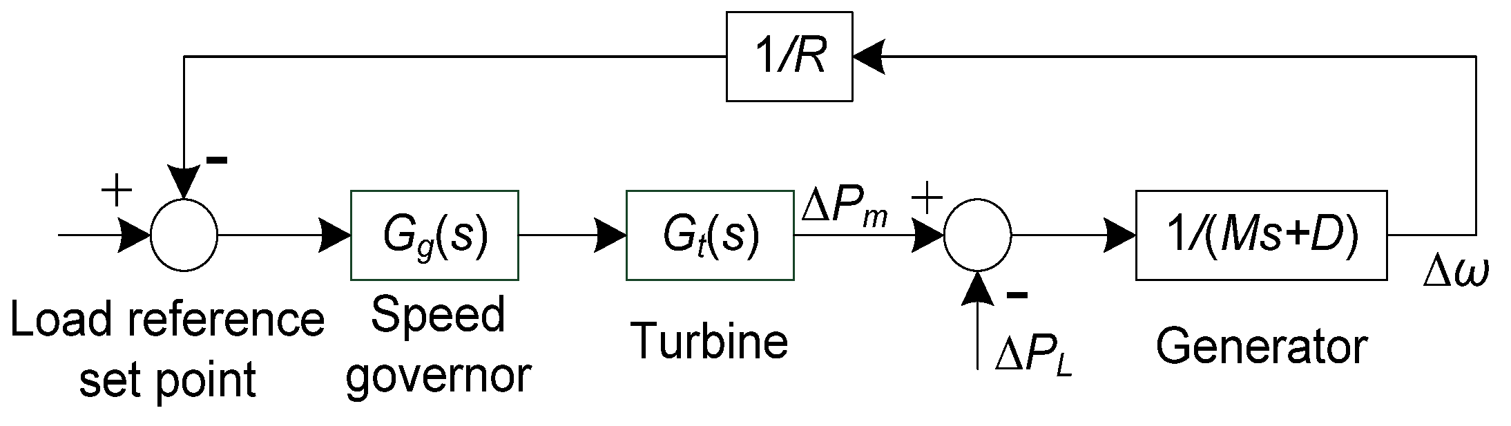
In a power system, real-time balance between generation and load is a fundamental requirement for its stable operations. However, some disturbances, such as a sudden drop of generation or short-circuit faults, will cause the mismatch between the two sides bringing damage to the facilities and instability to the power system [1]. Power system frequency is an accurate indicator for generation-load balance. The primary frequency control operates at a time-scale of seconds and uses a speed governor to adjust the mechanical power responding to the frequency deviation. The secondary frequency control operates at a time-scale of minutes and regulates the frequency according to the area control error (ACE) [2]. Traditionally, these two types of control are implemented on the generation side.

Relying solely on the generation side is not sufficient for frequency control. Conventional generating units are of high wear-and-tear cost and low thermal efficiency when responding to control signals in intervals of seconds [3,4]. With the environmental cost to be accounted for, reserve provision from generation, especially fossil-fueled generators, will be much more expensive. The large-scale integration of intermittent energy sources [5,6,7], e.g., wind and solar energy, will cause high variety and uncertainty in power outputs because of the stochastic nature of weather conditions [8,9,10]. Supplementary to the generation side, resources from the load side have the potential to provide low cost and fast responsive regulation.

The feasibility and efficiency of load control have been justified [11,12,13,14]. Direct load control (DLC) is a centralized scheme that is exerted directly by the control center for large-scale industrial loads [15,16,17]. As opposed to DLC, load control through small-scale residential and commercial loads is implemented on disperse end-users [18,19]. Thermostatically controlled loads (TCLs), e.g., air conditioners, heat pumps and refrigerators, are good options for primary frequency control because of their inherent heat capacity [20]. Compared with DLC, decentralized control through TCLs is much more flexible. Moreover, TCLs, especially air conditioners take a large proportion in load portfolio. For instance, in China, the proportion of air conditioners in peak power is almost 30%–40% during summer and grows year by year [21]. Consequently, air conditioners can take an active role for frequency control [22].

The fast advancement of smart grid technologies provides a gradually open platform for electricity users. Almost simultaneously, the smart home domain attracts building designers, telecommunication suppliers and appliance manufactures to join in to make home appliances connected and controlled flexibly [23]. Active participation of residential air conditioners in power system control appropriately interlinks the two smart domains, which can be implemented in an economical way.

The feasibility and effectiveness of air conditioners participating in power system operation have been demonstrated by recent research and field programs [24,25,26,27,28,29]. Studies in [24,25] verified the technical feasibility of air conditioners to participate in frequency control, which requires fast response. More and more utility companies carry out demand response programs involving residential air conditioners, e.g., the SmartAC program of Pacific Gas & Electric Company (PG&E) [26,27], the energy smart thermostat program by Southern California Edison [28] and the smart thermostat program at San Diego Gas & Electric Company [29].

Two mechanisms for air conditioners participating in frequency control are available: (1) directly switch ON/OFF and (2) modulation of temperature setting. In [14], a primary frequency control strategy by switching ON/OFF of demand-side devices was proposed. A frequency control scheme was demonstrated in [16] by adjusting temperature set points of air conditioners in high-density residential buildings. Two types of logics were respectively developed in [19] by directly switching ON/OFF or modulating temperature set points. Compared with the first mechanism, the second one is much more flexible and causes less negative impacts on users’ comfort. Many of the current control designs focus on manipulation of loads in a centralized way by using a general dynamic equation to describe the collective thermodynamics of loads [19,20]. The decentralized load control strategies were also studied. A decentralized primary-dual algorithm was proposed for optimal load control in [4,30].

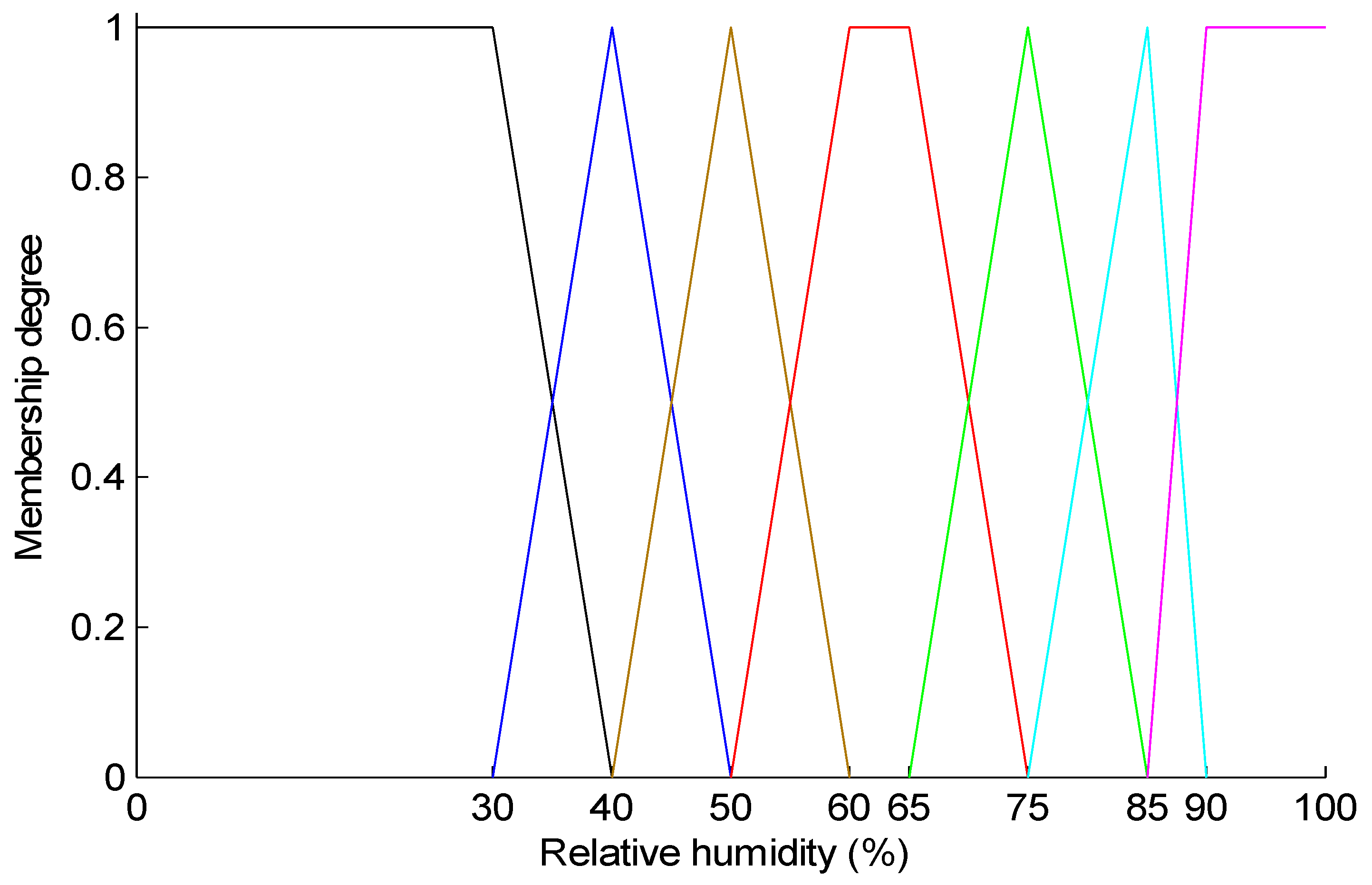
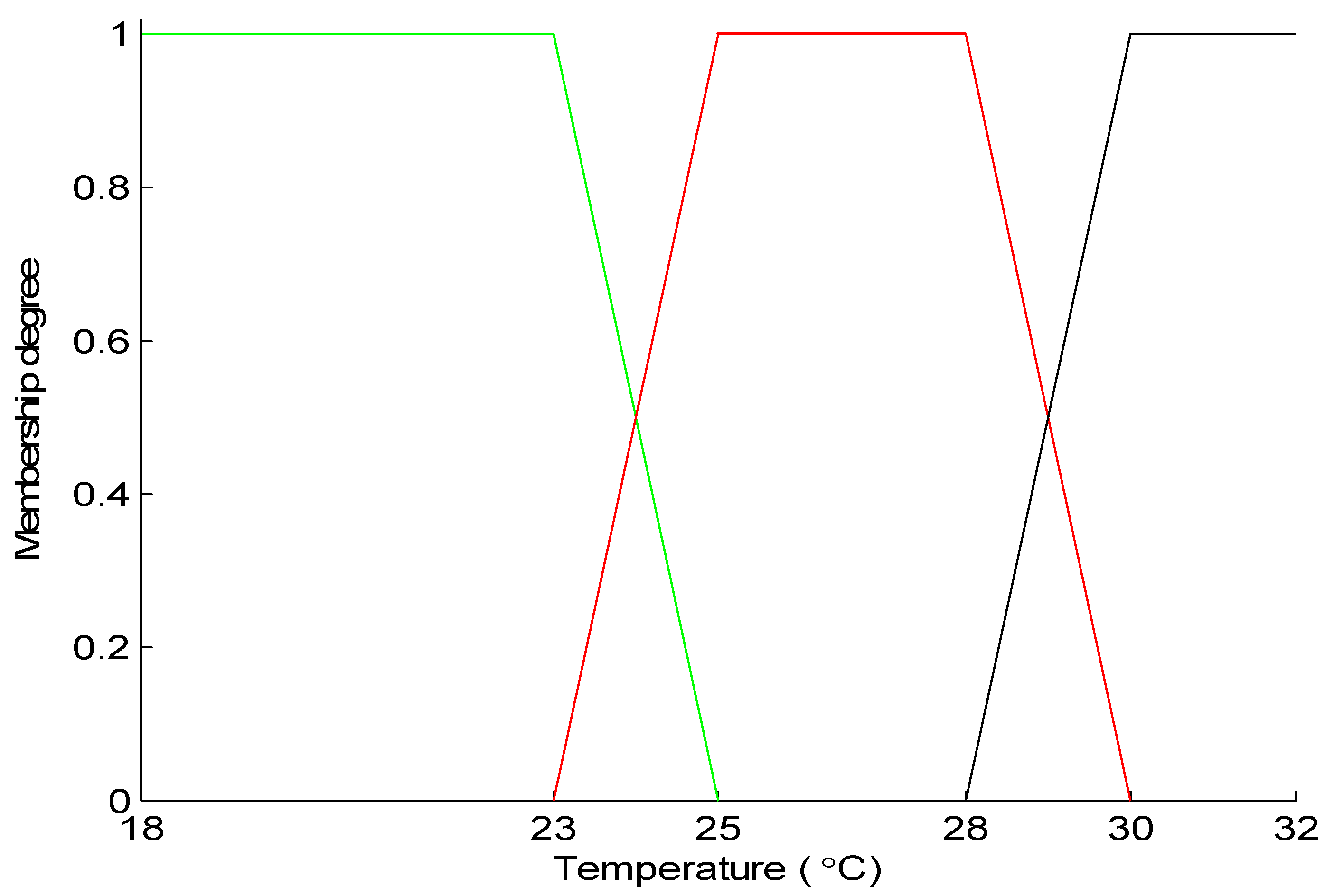
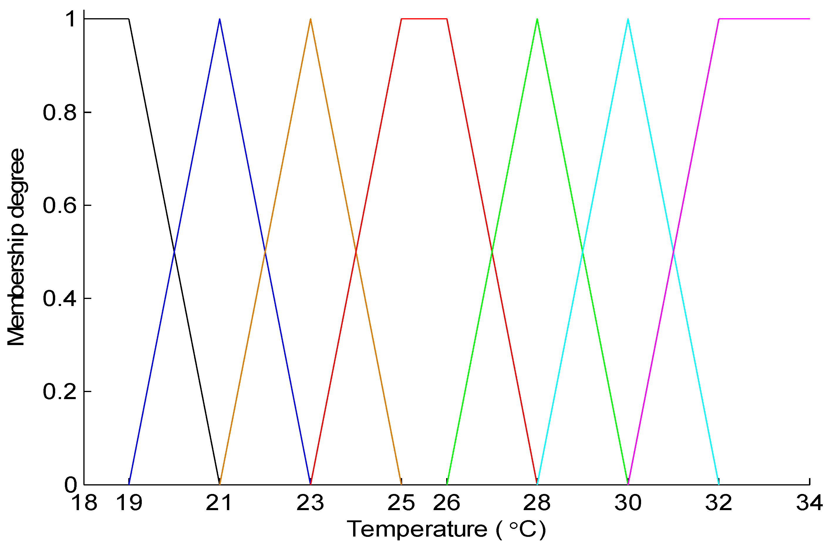
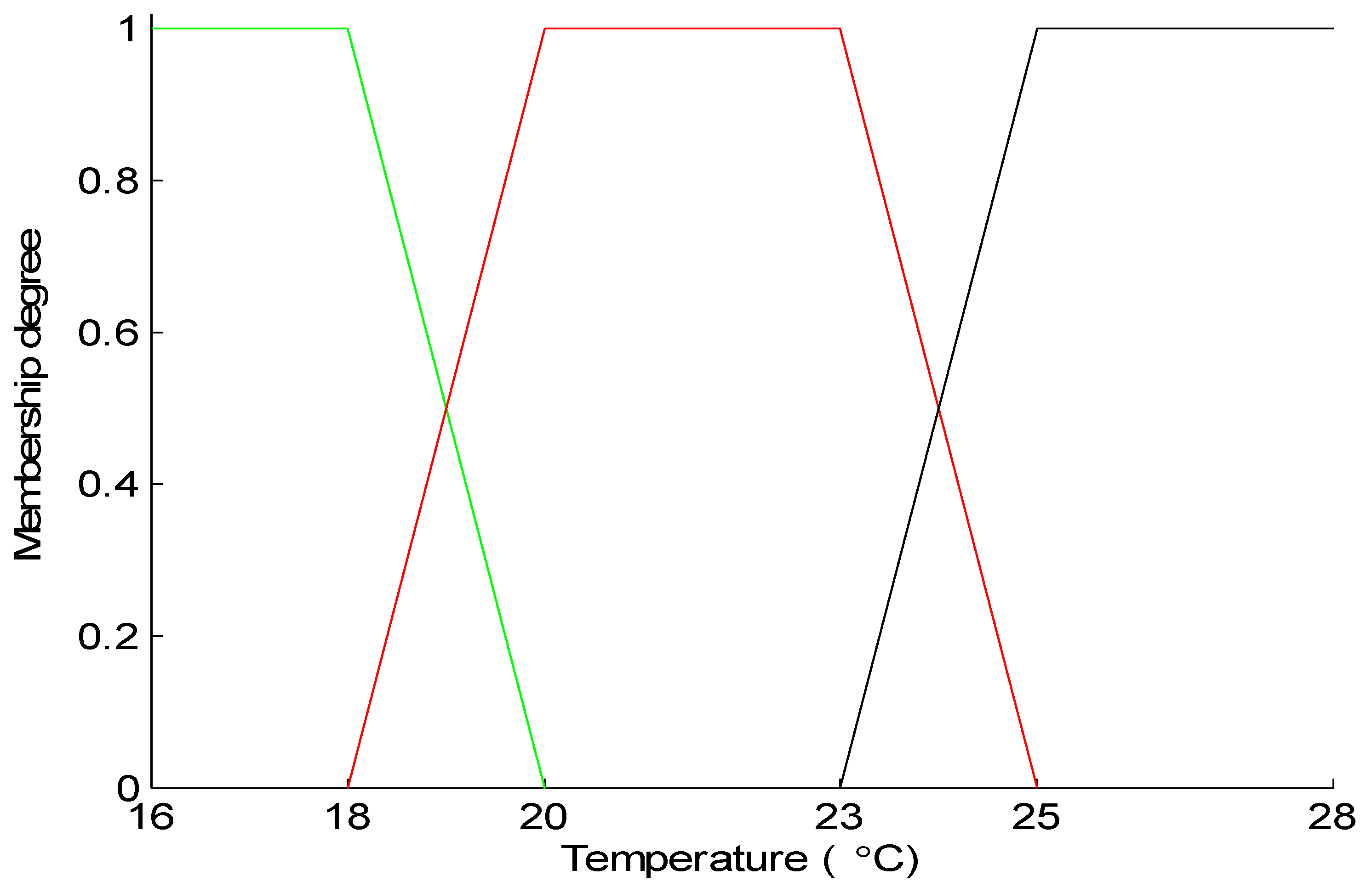
For air conditioners, the end-use utility is evaluated mainly by users’ thermal comfort. Various factors may influence human’s thermal feelings, in which temperature and relative humidity take the largest part for indoor users [31]. In general, humans feel more comfortable when the temperature is between 24 °C and 27 °C, while relative humidity is between 55% and 70% in summer [32,33,34,35,36]. Accounting for the user’s thermal comfort, the accurate description of conditioned space is required. First-order, second-order and third-order models were built, respectively, in [37,38,39] to depict thermodynamics of the conditioned space. In [30], the control strategy accounts for the utility of loads, but it focuses on the group’s characteristic rather than on each individual’s.

Air conditioners can actively respond to power system dynamics. Efforts have been made in the field of dynamics modeling. A single-generator power system model was used in [4] to test the feasibility and efficiency of load control, which is too simplified and less accurate. A classical multi-generator model was introduced in [3], which simplifies the network by grouping each generator bus with its nearby load buses. Since load buses are eliminated, the model is not able to accurately depict load characteristics. The structure preserving model is required with load buses retained [30]. Most of previous studies adopted DC power flow to describe the connectivity between buses, ignoring the influence of voltage characteristics on system dynamics [3,4,18,19].

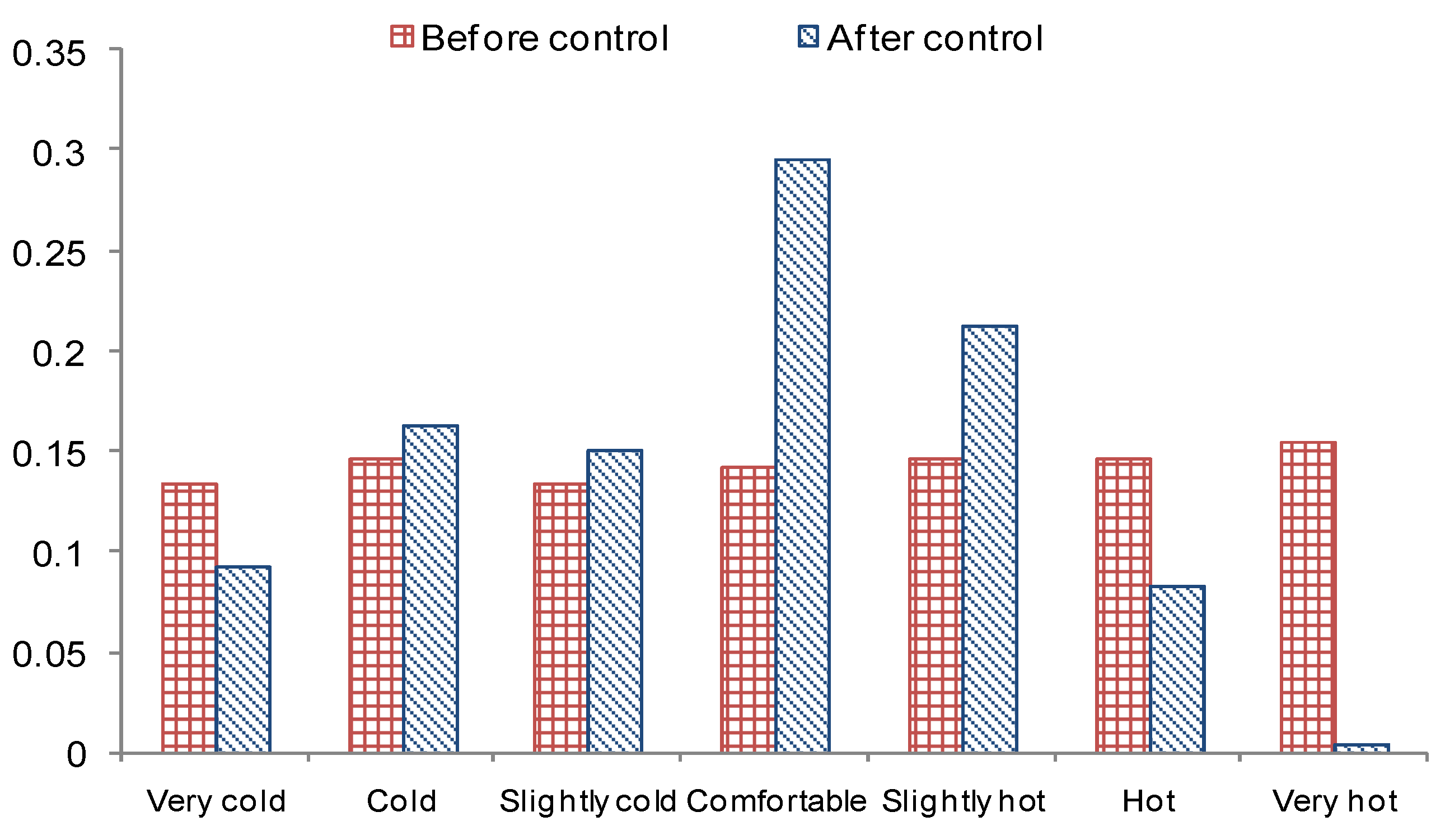
In this paper, we propose a strategy to facilitate the active participation of air conditioners. To evaluate users’ thermal comfort, fuzzy mathematics is employed to establish membership functions for various temperature and relative humidity values. The states of air conditioners are described by a third-order model, with its parameters sampled by using the Monte Carlo simulation method. When a disturbance occurs, the temperature set points of air conditioners will be adjusted in response to the degree of frequency deviation while keeping users’ thermal comfort within the appropriate range. A structure preserving model is applied to multi-bus power system, with both generator and load buses retained. Full AC power flow is adopted instead of DC power flow.

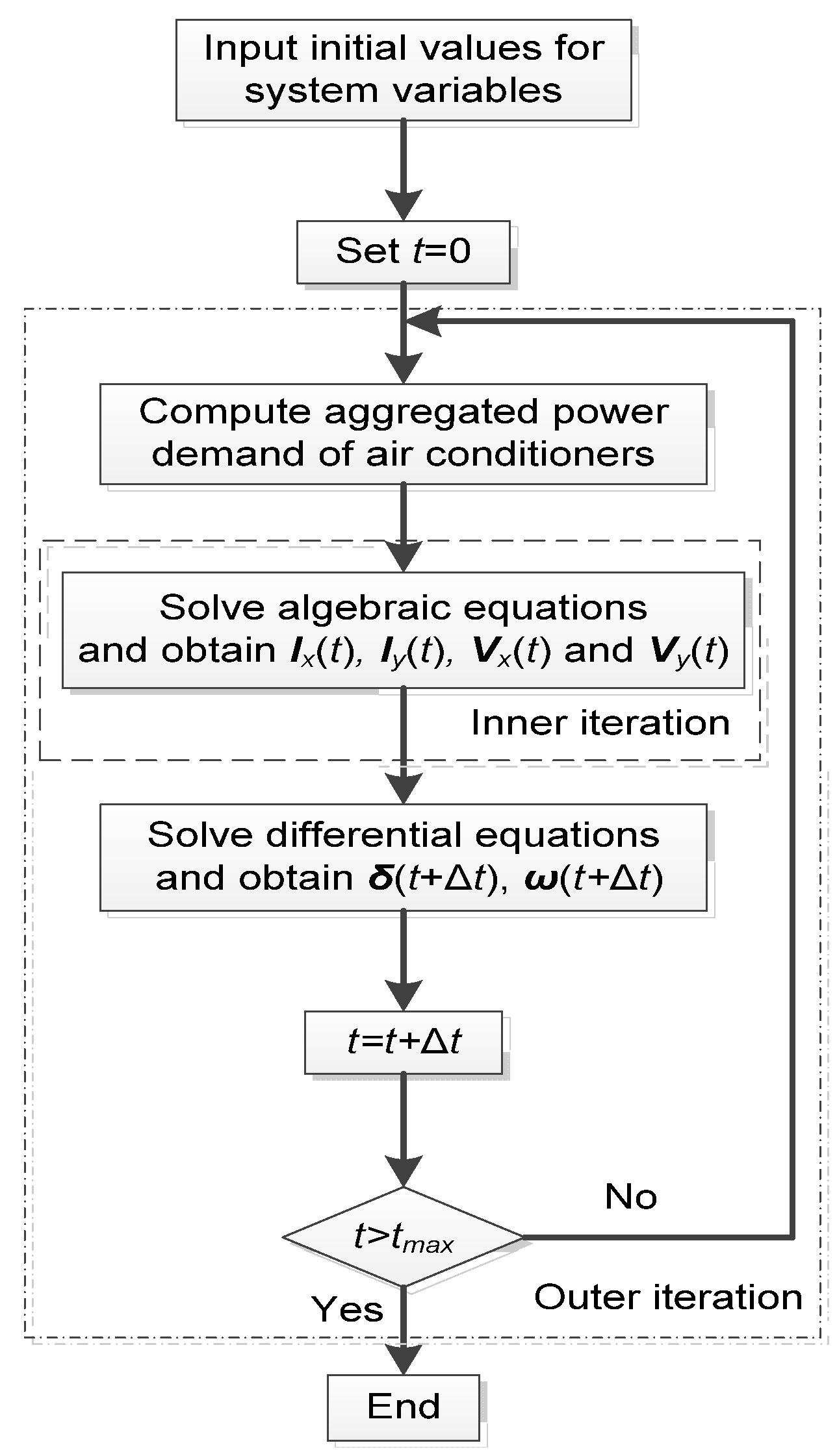
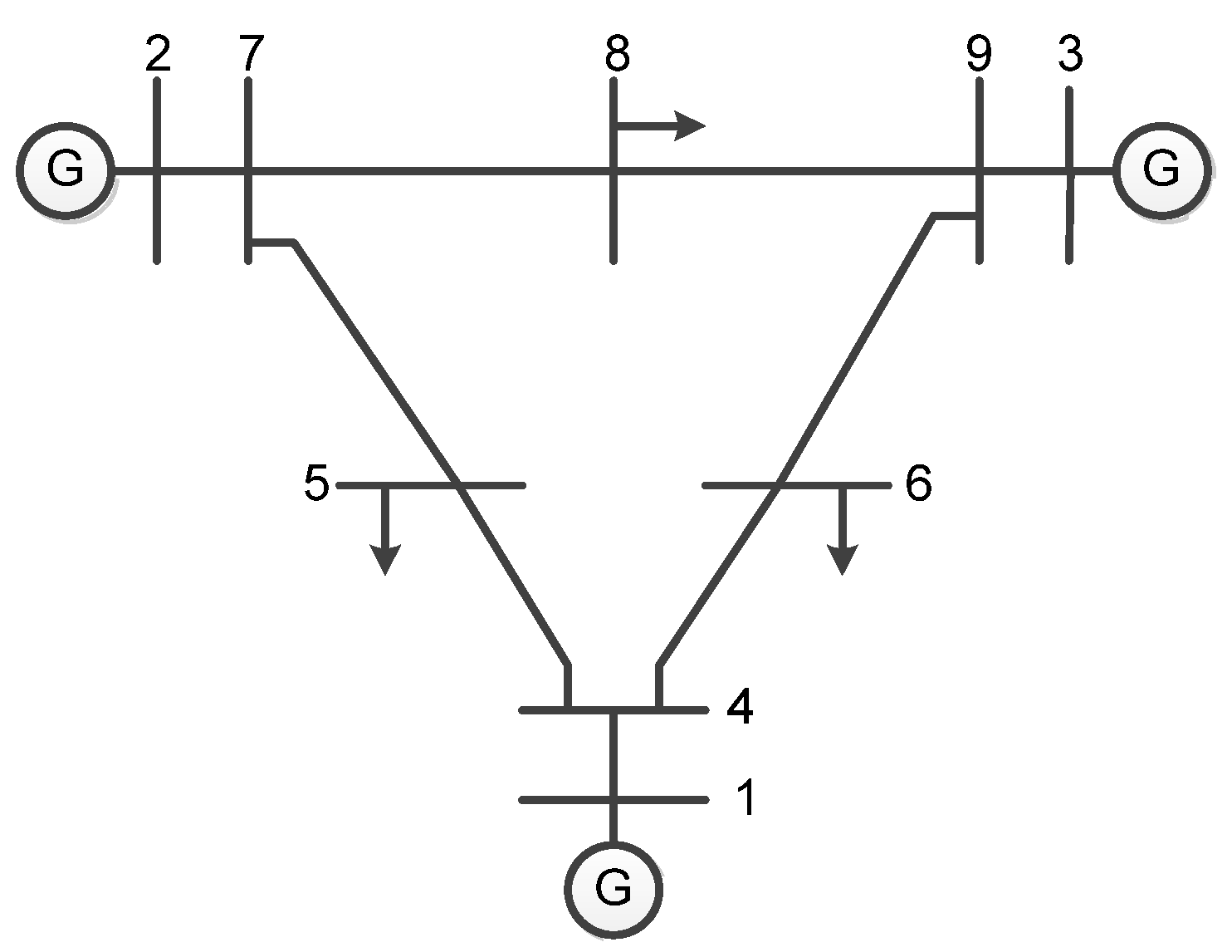
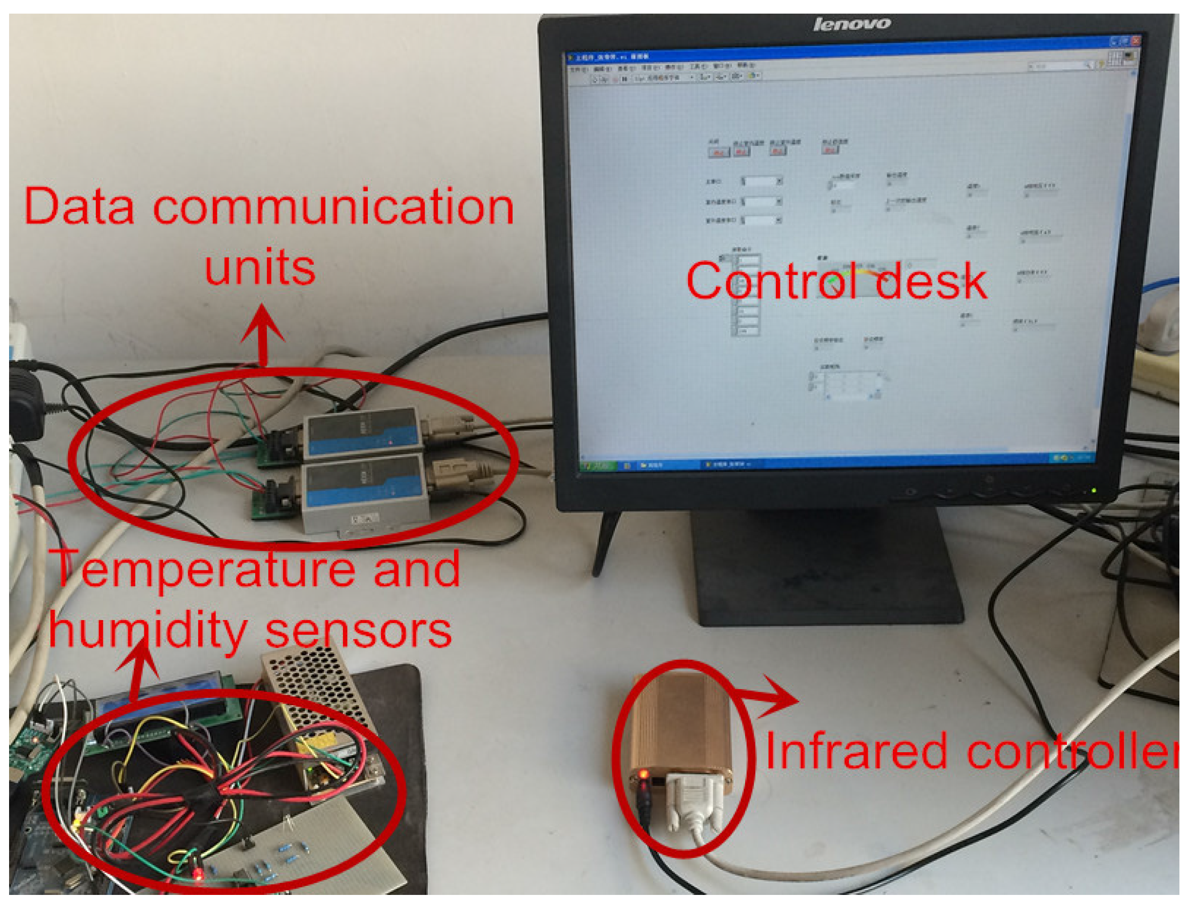
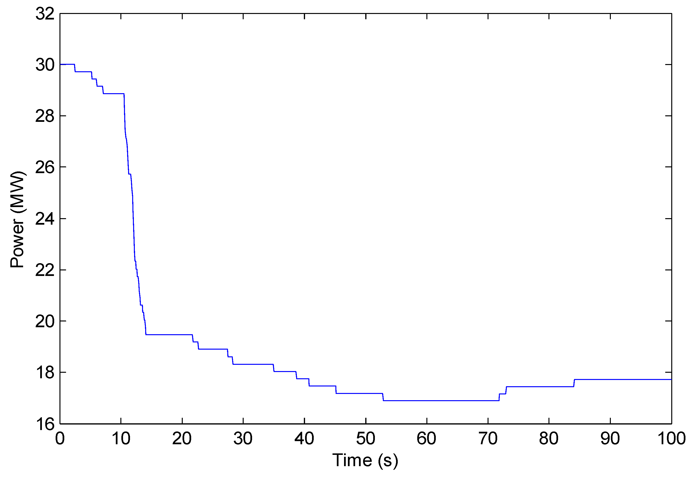
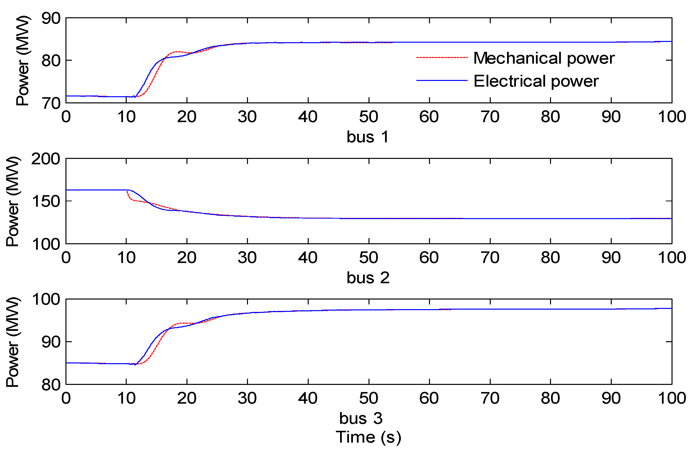
The remainder of this paper is organized as follows. Section 2 proposes a decentralized control law for air conditioners accounting for individual user’s thermal comfort. Section 3 models power system dynamics with the aggregation of air conditioners integrated. Section 4 presents results of case studies. Conclusions are drawn in Section 5.

2. Fuzzy Rule Based Decentralized Control for Frequency Regulation

2.1. Fuzzy Evaluation of Human Thermal Comfort

Thermal comfort is the subjective evaluation of occupants’ satisfaction with the thermal environment. It is influenced by multiple factors such as ambient temperature, relative humidity, wind velocity and solar radiation. For indoor occupants, temperature and relative humidity are two major factors. It is difficult to rank thermal comfort precisely with crisp boundaries. Fuzzy mathematics is an appropriate tool for assessment of thermal comfort. A comprehensive fuzzy algorithm involving indoor temperature and relative humidity is proposed to evaluate occupants’ thermal comfort.

Let χ = {very low, low, slightly low, moderate, slightly high, high, very high} stand for the domain of temperature ranks. Each rank is depicted by its own membership function shown in Figure 1. Triangular and trapezoid functions are used. The membership degree of a point x with respect to a triangular function defined in the interval [α, γ] and middle value in β is obtained as:

$${\mu }_{Triangular}(x)=\{\begin{array}{ll}\frac{x-\alpha }{\beta -\alpha },& \text{if }\alpha \le x\le \beta \\ 0,& \text{if }\alpha \text{>}x\text{ or }\gamma \text{<}x\\ \frac{\gamma -x}{\gamma -\beta },& \text{if }\beta \le x\le \gamma \end{array}$$

(1)

The membership degree of a point x with respect to a trapezoid function defined in the interval [α, γ] and middle values in β and φ (β < φ) is obtained as:

$${\mu }_{Trapezoid}(x)=\{\begin{array}{ll}\frac{x-\alpha }{\beta -\alpha },& \text{if }\alpha \le x\le \beta \\ 1,& \text{if }\beta \text{<}x\text{<}\phi \\ \frac{\gamma -x}{\gamma -\phi },& \text{if }\phi \le x\le \gamma \\ 0,& \text{ otherwise}\end{array}$$

(2)

Let σ = {very dry, dry, slightly dry, temperate, slightly wet, wet, very wet} stand for the domain of relative humidity ranks. Each rank is depicted by its own membership functions of triangular or trapezoid form as shown in Figure 2. The unit of humidity is g/m³ and the relative humidity is expressed in the form of percentage as the ratio of the water vapor density to the saturation water vapor density, which is used in this paper.

The mutual influence of temperature and relative humidity on thermal comfort is within a fuzzy domain. Human’s sensitivity to relative humidity is associated directly with temperature. When temperature is low, relative humidity has small influence on thermal comfort. However, when temperature rises, the influence of relative humidity will increase. Let ρ = {small, medium, large} stand for the domain of relative humidity influence rank. As shown in Figure 3, trapezoid membership functions are adopted for various relative humidity influence ranks. Once the temperature value is known, the influence rank of relative humidity will be obtained.

Figure 1. Temperature membership functions in summer.

Figure 1. Temperature membership functions in summer.

Figure 2. Relative humidity membership functions.

Figure 2. Relative humidity membership functions.

Let λ = [λ₁, λ₂] be the weight set for temperature and relative humidity, respectively, which satisfies

$${\lambda }_1+{\lambda }_2=1$$

(3)

where λ₁ weighs the influence of temperature on thermal comfort and λ₂ weighs the influence of relative humidity. Note that λ₂ is different for three influence ranks shown in Figure 3. When the influence rank of relative humidity is obtained, the weight set λ can be determined.

Figure 3. Relative humidity influence membership functions in summer.

Figure 3. Relative humidity influence membership functions in summer.

When temperature and relative humidity values are provided, the thermal comfort can be evaluated as

$$\begin{array}{ll}H& =\left[{\lambda }_1,{\lambda }_2\right]\left[\begin{array}{ccccccc}{\mu }_{11}& {\mu }_{12}& {\mu }_{13}& {\mu }_{14}& {\mu }_{15}& {\mu }_{16}& {\mu }_{17}\\ {\mu }_{21}& {\mu }_{22}& {\mu }_{23}& {\mu }_{24}& {\mu }_{25}& {\mu }_{26}& {\mu }_{27}\end{array}\right]\\ & =\left[\begin{array}{ccccccc}{h}_1& h_2& h_3& h_4& h_5& h_6& h_7\end{array}\right]\end{array}$$

(4)

where μ_1j is the jth temperature membership degree and μ_2j is the jth relative humidity membership degree (j = 1, 2,…,7). Ranks of the comprehensive thermal comfort are {very cold, cold, slightly cold, comfortable, slightly hot, hot, very hot}. The thermal comfort rank is defuzzified by the maximum operator:

$$h_{\text{max}}=\text{max}\{h_1,h_2,h_3,h_4,h_5,h_6,h_7\}$$

(5)

For instance, if h_max = h₄, the thermal comfort rank is “comfortable”.

2.2. Decentralized Control Design for Frequency Regulation

Local measurements enable each individual air conditioner to sense frequency deviation from the nominal value. When the frequency reaches the limit value of normal range, controller of the air conditioner will adjust its temperature set point to regulate power demand. The adjustment of the temperature set point accounts for the user’s thermal comfort evaluated by the fuzzy algorithm in Section 2.1.

In practice, under-frequency load shedding (UFLS) is a special control scheme for power system stability, which will cause a great cost once triggered. A frequency value is set for UFLS under which load shedding should be activated [40,41]. Compared with UFLS, the control scheme proposed in this paper is a “soft” one with much less cost and it will respond to the abnormal frequency earlier than the activation of UFLS. As shown in Figure 4, the activation frequency range of the proposed scheme is

$$\Delta f_{range}=f_u-f_l$$

(6)

where f_u is the activation frequency value of UFLS and f_l is the lowest value of normal frequency.

Figure 4. Activation frequency range.

Figure 4. Activation frequency range.

Thermal comfort rank can be evaluated at a certain temperature and relative humidity. In summer, if the thermal comfort rank is “very cold”, “cold” or “slightly cold”, the temperature will be raised to a higher value at which the rank is “comfortable”. Otherwise, if the rank is among “comfortable”, “slightly hot”, “hot” or “very hot”, the temperature should not be adjusted. In winter, the adjustment is in the reverse direction. Relative humidity is treated as constant during a control span, which is reasonable since the span is short. The span is the time duration of an air conditioner from OFF state to ON state after it responds to the control signal, which is determined by the time constant of thermal mass in the conditioned room. The maximum temperature adjustment is

$$\Delta T_{\text{max}}=T_{new}-T_{old}$$

(7)

where T_old is the initial temperature; and T_new is the higher temperature.

For each air conditioner, the actual temperature adjustment responding to frequency deviation is

$$\Delta T_{set}=\frac{\Delta T_{\text{max}}}{\Delta f_{range}}\Delta f$$

(8)

where Δf is actual frequency deviation.

Within the activation frequency range, the proposed control scheme will regulate air conditioners in response to the frequency deviation while maintaining users’ thermal comfort. However, when the frequency value is lower than f_u, the air conditioners will be switched off directly.

2.3. Aggregation of Air Conditioners’ Response

Air conditioners are of periodic on/off working characteristics. The temperature set point is the boundary for an air conditioner to switch from on to off or vice versa. By increasing the temperature set point, the air conditioner tends to be off. Power demand will decrease significantly if a large number of air conditioners switch off within a short time range.

Assume that the power system is working at an operating point where generation and load are in balance. Then, a sudden generation drop occurs and consequently the system frequency decreases. Each air conditioner responds to the frequency deviation through temperature set point adjustment according to the control law in Equation (8).

Changing the temperature set point will influence states of an air conditioner and its conditioned space, which can be depicted by a dynamical model [39]

$$\begin{array}{l}\dot{\mathit{x}}=\mathit{A}\mathit{x}+\mathit{B}\mathit{u}\\ \mathit{y}=\mathit{C}\mathit{x}\end{array}$$

(9)

where x, u, y, A, B and C are detailed in Appendix A.

The Monte Carlo simulation method is applied to the aggregation of air conditioners’ response. Each air conditioner in the control group is treated as a sample with its parameters randomized. The aggregated power demand of the group of air conditioners is

$$P_{ac}(t)={\displaystyle \sum _{j\in \psi }{p}_j}(t)$$

(10)

where ψ = {1, 2, … , N} represents individual air conditioners; and p_j(t) is the power demand of air conditioner j at time t.

Note that the following three aspects of using air conditioners for frequency control are considered but not directly treated in this paper:

(1)

Energy payback phenomenon is caused by the synchronization of air conditioners during the recovery process. A careful recovery strategy can be used to avoid the phenomenon [42,43].

(2)

To attract more electricity users to participate in active load control, a power grid can design various incentive tools. Incentive-based demand response programs have been carried out in recent years [44,45,46]. Users can contract with the power grid on the compensation and award packages for their comfort loss and contributions for the power grid.

(3)

Conventionally, generating units supply spinning reserves and non-spinning reserves for the power system. At demand peak periods, the cost of maintaining high reserve level is very large. Air conditioners are capable of providing reserves with much lower cost than generating units. The economic saving through the proposed strategy can be quantified by the value of reduced reserve capacity procured from the generation side.

3. Power System Dynamics Model

3.1. Dynamical Model of Generating Units

A governor-turbine-generator model is used to represent a generating unit as shown in Figure 5, which accounts for primary frequency regulation of the unit.

Figure 5. Generating unit model.

Figure 5. Generating unit model.

Dynamics of the generator can be described by the swing equations as

$$\{\begin{array}{l}\frac{\text{d}\delta }{\text{d}t}={\omega }_s(\omega -1)\\ M\frac{\text{d}\omega }{\text{d}t}=P_m-P_e\end{array}$$

(11)

where δ is generator rotor angle; ω is rotor angle speed; ω_s is nominal angle speed; P_m and P_e are, respectively, mechanical power and electrical power; and M is angular momentum of the generator. Electrical power can be derived by

$$P_{\text{e}}=P_L+D\omega$$

(12)

where D is damping coefficient; and P_L is power demand of load.

The turbine block has the transfer function as

$$G_t(s)=\frac{1+s{F}_{HP}{T}_{RH}}{(1+s{T}_{CH})(1+s{T}_{RH})}$$

(13)

where F_HP is intermediate pressure cylinder mechanical ratio; and T_CH and T_RH are volume effect time constants.

The transfer function of the speed governor is

$$G_g(s)=\frac{1}{1+s{T}_G}$$

(14)

where T_G is governor time constant. As shown in Figure 5, R is the gain of the feedback loop for the governor, which determines the speed droop characteristic.

3.2. Network Model

A power network is modeled by a graph ζ = {ν, ε}, where ν = {1, 2, … , n} is the set of buses and ε is the set of transmission lines connecting the buses. Bus voltage equations of the power network can be expressed as

$$\mathit{Y}\mathit{V}=\mathit{I}$$

(15)

where I and V are injection current vector and bus voltage vector, respectively; and Y is nodal admittance matrix.

A power network has three types of buses including generator buses, load buses and contact buses. The injection currents at a generator bus i can be described as

$$\left[\begin{array}{l}{I}_{xi}\\ I_{yi}\end{array}\right]=\left[\begin{array}{l}\frac{\text{sin}{\delta }_i}{X_{di}^{\prime }}\\ -\frac{\text{cos}{\delta }_i}{X_{di}^{\prime }}\end{array}\right]E_i^{\prime }-\left[\begin{array}{cc}0& \frac{1}{X_{di}^{\prime }}\\ -\frac{1}{X_{di}^{\prime }}& 0\end{array}\right]\left[\begin{array}{l}{V}_{xi}\\ V_{yi}\end{array}\right]$$

(16)

where I_xi and I_yi are, respectively, real and imaginary part of injection current; V_xi and V_yi are, respectively, real and imaginary part of voltage; $X_{di}^{\prime }$ is direct-axis transient reactance; and $E_i^{\prime }$ is electromotive force of the generator.

At contact buses, the net injection currents are zero:

$$\left[\begin{array}{l}{I}_{xi}\\ I_{yi}\end{array}\right]=0$$

(17)

A load bus may consist of conventional loads and aggregation of air conditioners. The injection currents at load bus i are presented by

$$\left[\begin{array}{l}{I}_{xi}\\ I_{yi}\end{array}\right]=\left[\begin{array}{l}{I}_{xi\_c}\\ I_{yi\_c}\end{array}\right]+\left[\begin{array}{l}{I}_{xi\_ac}\\ I_{yi\_ac}\end{array}\right]$$

(18)

where I_{xi_c} and I_{yi_c} are, respectively, real and imaginary part of injection current of conventional loads; and I_{xi_ac} and I_{yi_ac} are corresponding values of air conditioners, respectively. The conventional loads can be described by their static characteristics and dynamic characteristics, respectively.

Quadratic polynomial is usually used to describe the static characteristics of loads

$$\{\begin{array}{l}{P}_L=P_{L(0)}[a_P{(\frac{V_L}{V_{L(0)}})}^2+b_P(\frac{V_L}{V_{L(0)}})+c_P]\\ Q_L=Q_{L(0)}[a_Q{(\frac{V_L}{V_{L(0)}})}^2+b_Q(\frac{V_L}{V_{L(0)}})+c_Q]\end{array}$$

(19)

where P_L(0) and Q_L(0) are pre-disturbance value of real power and reactive power of a load, respectively; and V_L(0) is pre-disturbance value of voltage at the load bus. The load comprises constant impedance, constant current and constant power proportions and a, b, c are corresponding coefficients satisfying

$$\{\begin{array}{l}{a}_P+b_P+c_P=1\\ a_Q+b_Q+c_Q=1\end{array}$$

(20)

The injection currents of the constant impedance proportion are

$$\left[\begin{array}{l}{I}_{xi\_c}\\ I_{yi\_c}\end{array}\right]=\left[\begin{array}{cc}\frac{-P_{i\_c(0)}}{V_{i(0)}^2}& \frac{-Q_{i\_c(0)}}{V_{i(0)}^2}\\ \frac{Q_{i\_c(0)}}{V_{i(0)}^2}& \frac{-P_{i\_c(0)}}{V_{i(0)}^2}\end{array}\right]\left[\begin{array}{l}{V}_{xi}\\ V_{yi}\end{array}\right]$$

(21)

where P_{i_c(0)} and Q_{i_c(0)} are, respectively, pre-disturbance value of real power and reactive power; and V_i(0) is pre-disturbance value of voltage. Constant current and constant power proportions are also readily to be included in the power network model.

Dynamic characteristics of conventional loads are usually associated with induction motors, which can be described as

$$\left[\begin{array}{l}{I}_{xi\_m}\\ I_{yi\_m}\end{array}\right]=-\left[\begin{array}{l}\frac{R_{i\_m}}{R_{i\_m}^2+X_{i\_m}^2}\\ \frac{-X_{i\_m}}{R_{i\_m}^2+X_{i\_m}^2}\end{array}\right]E_{i\_m}^{\prime }$$

(22)

where $E_{i\_m}^{\prime }$ is the transient electromotive force of the induction motor; and R_{i_m} and X_{i_m} are equivalent resistance and reactance, respectively.

Real power and reactive power of the aggregation of air conditioners will change with time in response to frequency dynamics. Consequently, the relationship between the injection current and bus voltage is nonlinear. The injection currents of the aggregation of air conditioners can be described as

$$\{\begin{array}{l}{I}_{xi\_ac}=-\frac{P_{i\_ac}{V}_{xi}+Q_{i\_ac}{V}_{yi}}{V_{xi}^2+V_{yi}^2}\\ I_{yi\_ac}=-\frac{P_{i\_ac}{V}_{yi}-Q_{i\_ac}{V}_{xi}}{V_{xi}^2+V_{yi}^2}\end{array}$$

(23)

where P_{i_ac} and Q_{i_ac} are real power and reactive power of the aggregation of air conditioners, respectively.

When I_xi, I_yi, V_xi and V_yi are determined, the electrical power of generator i can be computed as

$$P_{ei}=I_{xi}{V}_{xi}+I_{yi}{V}_{yi}$$

(24)

3.3. Solving Dynamics

The dynamical model for the power system is constructed by integrating dynamical equations of air conditioners in Equations (9) and (10) and generating units in Equations (11)–(14) with the network model in Equation (15). The numerical integration method is applied to solving the differential-algebraic equations.

Since the relationship between injection current and voltage is nonlinear in Equation (23), an iteration process should be used to solve it. In each iteration k, the correction formula of voltage variables is

$$\left[\begin{array}{l}\Delta {\mathit{I}}_x^{\left(k\right)}\\ \Delta {\mathit{I}}_y^{\left(k\right)}\end{array}\right]\text{=}\left[\begin{array}{cc}{\mathit{H}}^{\left(k\right)}& {\mathit{N}}^{\left(k\right)}\\ {\mathit{M}}^{\left(k\right)}& {\mathit{L}}^{\left(k\right)}\end{array}\right]\left[\begin{array}{l}\Delta {\mathit{V}}_x^{\left(k\right)}\\ \Delta {\mathit{V}}_y^{\left(k\right)}\end{array}\right]$$

(25)

where

$$\{\begin{array}{l}{H}_{ij}^{(k)}=\partial I_{xi}^{(k)}/\partial V_{xj}^{(k)}-G_{ij}\\ N_{ij}^{(k)}=\partial I_{xi}^{(k)}/\partial V_{yj}^{(k)}+B_{ij}\\ M_{ij}^{(k)}=\partial I_{yi}^{(k)}/\partial V_{xj}^{(k)}-B_{ij}\\ L_{ij}^{(k)}=\partial I_{yi}^{(k)}/\partial V_{yj}^{(k)}-G_{ij}\end{array}$$

(26)

where G_ij and B_ij are the real and imaginary part of nodal admittance, respectively.

At bus i, the error items for injection currents are

$$\{\begin{array}{l}\Delta I_{xi}^{(k)}=I_{xi}^{(k)}-{\displaystyle \sum _{m\in i}(G_{im}{V}_{xm}^{(k)}-B_{im}{V}_{ym}^{(k)})}\\ \Delta I_{yi}^{(k)}=I_{yi}^{(k)}-{\displaystyle \sum _{m\in i}(G_{im}{V}_{ym}^{(k)}+B_{im}{V}_{xm}^{(k)})}\end{array}$$

(27)

where m ∈ i represents each bus that connects with bus i by a transmission line.

A two stage iterative scheme is designed as shown in Figure 6. The inner iteration process is to solve voltage variables at the load bus with the aggregation of air conditioners. The outer iteration process is for solving dynamics of generating units and air conditioners. An alternating method is adopted for the outer iteration process involving both differential and algebraic equations. The modified Euler algorithm is used for numerical integration.

Figure 6. Solving process for power system dynamics.

Figure 6. Solving process for power system dynamics.

4. Case Studies

4.1. Experimental Results of Decentralized Control Design

We design an experiment to verify the effectiveness of the fuzzy rule based decentralized control for an air conditioner. The experiment was conducted in a winter season, when the air conditioner was operated in the heat pump mode. Except for the setting parameters, the control law is the same with that in summer. As shown in Figure B1 of Appendix B, the temperature rank membership functions in winter are different from those in summer. However, the relative humidity rank membership functions are the same with those in summer. The relative humidity influence rank membership functions are not same with those in summer, which are displayed in Figure B2 of Appendix B. Weights of temperature and relative humidity for three influence ranks are shown in Table 1.

Table 1. Weight proportions.

Weights	Relative humidity influence ranks
	Small	Medium	Large
λ1	0.9	0.8	0.6
λ2	0.1	0.2	0.4

Table 1. Weight proportions.

Weights	Relative humidity influence ranks
	Small	Medium	Large
λ1	0.9	0.8	0.6
λ2	0.1	0.2	0.4

The test rig consists of an air conditioner, a power system state monitoring module, temperature and humidity sensors, data communication units, an infrared controller and a control desk, which is displayed in Figure 7 and Figure 8. In the experiment, the power system state monitoring module is responsible for measuring frequency, voltage, and current at the node where the air conditioner plugs into the power system. Two sensors are used to sense indoor temperature and relative humidity, respectively. The measurement data are transmitted to the control desk through data communication units. The infrared controller is the external agent for the air conditioner to regulate its temperature set point. A supervisory system runs in the control desk to make control decision and coordinate various modules, which was developed with LabVIEW. When the frequency deviates from the normal range, the control desk will determine the new temperature set point according to the control law in Section 2.2. The control signal then will be sent to the air conditioner via the infrared controller.

In this experimental setup, the cost of temperature-humidity sensors and power system frequency meter are about 20 RMB Yuan (3.2 dollars) and 10 RMB Yuan (1.6 dollars), respectively. It is feasible to expect that the expense will be affordable for such a module to be equipped in an air conditioner or installed separately.

Figure 7. Measurement, communication and control modules.

Figure 7. Measurement, communication and control modules.

Figure 8. Test rig.

Figure 8. Test rig.

As shown in Figure 9, a frequency signal is generated to emulate the typical characteristic curve of frequency dynamics caused by a power system disturbance. Assume that frequency initially keeps at its nominal value of 50 Hz and then a generation drop occurs at the 10-s instant. Driven by the imbalance between generation and load, frequency decreases from 50 Hz. After dropping to the lowest value, frequency recovers to a new steady state value. The frequency signal is fed into the test rig and sampled every 0.1 s to trigger the control flow. The experiment was conducted for 240 runs starting from various initial values of the indoor temperature that follow the uniform distribution between 13 °C and 29 °C. The assumption of uniform distribution intends to generally cover more indoor conditions, and is not limited to certain specific situations.

Figure 9. Frequency signal for experiment.

Figure 9. Frequency signal for experiment.

In each experimental run, the air conditioner will be controlled in response to the frequency signal in accordance with the proposed control law. If the thermal comfort rank at the initial temperature value is among “very hot”, “hot” or “slightly hot”, the temperature set point will be adjusted to decrease. Consequently, the indoor temperature will decrease since the air conditioner intends to switch off. However, if the thermal comfort rank at the initial temperature value is among “very cold”, “cold” or “slightly cold”, the air conditioner will not respond to the frequency deviation. From results of the 240 experimental runs, the distribution of various thermal comfort ranks is derived. As shown in Figure 10, the percentages of “very hot” and “hot” ranks decrease significantly, whereas the percentages of “comfortable” and “slightly hot” ranks increase most after control. However, the percentages of “very cold”, “cold” and “slightly cold” ranks change less. Table 2 lists the detailed percentage numbers. To summarize, the indoor temperature has a large probability to be moved to the rank of “comfortable” after control. The control design for the air conditioner has positive impact on the user’s thermal comfort.

Figure 10. Thermal comfort rank distribution.

Figure 10. Thermal comfort rank distribution.

Table 2. Thermal comfort rank distribution.

Thermal comfort ranks	Very cold	Cold	Slightly cold	Comfortable	Slightly hot	Hot	Very hot
Before control	0.133	0.146	0.133	0.142	0.146	0.146	0.154
After control	0.092	0.1625	0.150	0.296	0.2125	0.083	0.004

Table 2. Thermal comfort rank distribution.

Thermal comfort ranks	Very cold	Cold	Slightly cold	Comfortable	Slightly hot	Hot	Very hot
Before control	0.133	0.146	0.133	0.142	0.146	0.146	0.154
After control	0.092	0.1625	0.150	0.296	0.2125	0.083	0.004

4.2. Simulation Results of Test Power System

To examine the control performance on multi-machine, multi-bus power system, simulations are conducted on the IEEE 9-bus test system. The test system consists of nine buses, three generating units and three loads. The single line diagram of the test system is displayed in Figure 11. Parameters of generating units are given in Table 3. Simulations are programmed and run in MATLAB.

Figure 11. Single line diagram of the IEEE 9-bus test system.

Figure 11. Single line diagram of the IEEE 9-bus test system.

Table 3. Parameters of generating units.

Parameters	Values (s)	Parameters	Values(p. u.)
TG	0.2	D	1
TRH	7	R	0.05
TCH	0.3	FHP	0.3
M	10

Table 3. Parameters of generating units.

Parameters	Values (s)	Parameters	Values(p. u.)
TG	0.2	D	1
TRH	7	R	0.05
TCH	0.3	FHP	0.3
M	10

Assume that a total of 10,000 air conditioners are aggregated at bus 8. Each air conditioner responds in accordance with the decentralized control law proposed in Section 2. The aggregation of air conditioners’ response is conducted on the basis of random sampling. The typical values of thermal parameters characterizing air-conditioned indoor space are given in

Table A1. Thermal parameters of air-conditioned indoor space.

Parameters	Expectation	Variance
Cew	1.875 MJ/°C	0.03 MJ/°C
Cin	1.2 MJ/°C	0.03 MJ/°C
Ciw	3.1 MJ/°C	0.05 MJ/°C
Rgs	0.08 °C/W	0.0002 °C/W
Riw	0.01 °C/W	0.00002 °C/W
Rew	0.028 °C/W	0.00002 °C/W
Rcew	0.005 °C/W	0.00002 °C/W

and

Table A2. Thermal parameters of air-conditioned indoor space.

Parameters	Range (°C)	Parameters	Range (W)
Xext	[25,28]	Peq	[490,510]
Xin	[18,33]	Pe-w	[190,210]
Xiw	[20,30]	PHVAC	[2500,3000]
Xew	[24,27]
Xadj-r	[20,30]

of Appendix A. The parameters are randomly sampled, which follows the normal distribution (the parameters shown in Table A1) or uniform distribution (the parameters shown in Table A2).

The power system is stable before the disturbance, with its frequency fluctuating very slightly from the nominal value of 50 Hz. At the 10-s instant, a generation drop occurs at bus 2, which is simulated by regulating the steam valve opening U:

$$U(t)=\{\begin{array}{l}1\text{ p}.\text{ u}.0\le t<10\text{ s}\\ 0.5\text{ p}.\text{ u}.t\ge 10\text{ s}\end{array}$$

(28)

Then, the system frequency drops down from its nominal value. To mitigate the frequency drop, reserve resources are activated from both the generation side and load side. In this study, air conditioners are the major reserve resource from the load side. When the power balance is rebuilt between generation and load around the 40-s instant, the system frequency reaches a new steady state.

The participation of air conditioners improves the system frequency characteristics by lessening drop depth and lifting steady state, which is displayed in Table 4 and Figure 12. Six cases are studied representing various participation ratios of air conditioners, from zero (r = 0) to 50% (r = 0.5). The larger the ratio is, the more significant the improvement is. For instance, the lowest point of frequency drop, the nadir, is 49.49 Hz for the case of r = 0.3 while it is 49.31 Hz for the case of r = 0, i.e., no air conditioners participating. With the new steady state built, the frequency recovers to 49.71 Hz for the case of r = 0.3 compared with 49.59 Hz for the case of r = 0.

Table 4. Frequency characteristics.

Frequency (Hz)	Ratio of air conditioning demand in load at bus 8
	r = 0	r = 0.1	r = 0.2	r = 0.3	r = 0.4	r = 0.5
Lowest point	49.31	49.36	49.45	49.49	49.56	49.64
Steady state	49.59	49.62	49.68	49.71	49.73	49.81

Table 4. Frequency characteristics.

Frequency (Hz)	Ratio of air conditioning demand in load at bus 8
	r = 0	r = 0.1	r = 0.2	r = 0.3	r = 0.4	r = 0.5
Lowest point	49.31	49.36	49.45	49.49	49.56	49.64
Steady state	49.59	49.62	49.68	49.71	49.73	49.81

As displayed in Figure 13, aggregated power demand of air conditioners decreases since it is fairly sensitive to the system frequency, which services to the power rebalance between generation and load after disturbance. For the case of r = 0.3, the aggregated power demand is around 30 MW before disturbance. After the disturbance occurs at the 10-s instant, it decreases sharply in response to the frequency drop. At the 40-s instant, the aggregated power demand levels off to around 18 MW. The contribution of air conditioners is estimated to be 12 MW (= 30 MW−18 MW), which is about 40% of its baseline demand before disturbance.

Figure 12. Frequency dynamics.

Figure 12. Frequency dynamics.

Figure 13. The demand of air conditioners after the disturbance.

Figure 13. The demand of air conditioners after the disturbance.

As shown in Figure 14, generating units respond to the system frequency dynamics by regulating their mechanical power along with electrical power. Each unit is controlled locally to stabilize the rotor angle speed, with the regulation of its mechanical power contributing to compensate for the power imbalance caused by the disturbance. Mechanical power of the generating unit at bus 2 decreases because of the generation drop. Mechanical power of the unit at bus 1 (or bus 3) increases to compensate for the power deficit. The rebalance between mechanical power and electrical power is achieved at each generator bus around the 40-s instant when the frequency stabilizes to a steady state as shown in Figure 12.

Figure 14. Mechanical power and electrical power at generator buses 1, 2 and 3.

Figure 14. Mechanical power and electrical power at generator buses 1, 2 and 3.

5. Conclusions

This paper proposes a strategy for air conditioners participating in power system frequency regulation. According to the decentralized control law proposed, each air conditioner will respond to the frequency deviation by regulating its temperature set point while maintaining the user’s thermal comfort. A fuzzy algorithm is used to evaluate user’s thermal comfort. The population of air conditioners is aggregated through the Monte Carlo simulation method. A structure preserving model for power system is adopted with characteristics of aggregated air conditioners being depicted correctly, which is solved by an inner-outer iteration algorithm. Experimental and simulation results verify the effectiveness and performance of the proposed strategy for air conditioners to actively participate in power system frequency control.

References

1. Wang, X.; Song, Y.; Irving, M. Modern Power System Analysis, 1st ed.; Springer U.S.: New York, NY, USA, 2008. [Google Scholar]
2. Wood, A.J.; Wollenberg, B.F. Power Generation, Operation and Control, 2nd ed.; Wiley & Sons: New York, NY, USA, 1996. [Google Scholar]
3. Zhao, C.; Ufuk, T.; Low, S. Swing dynamics as primary-dual algorithm for optimal load control. In Proceedings of the IEEE 3rd International Conference on Smart Grid Communications, Tainan, Taiwan, 5–8 November 2012; pp. 570–575.
4. Zhao, C.; Ufuk, T.; Low, S. Optimal load control via frequency measurement and neighborhood area communication. IEEE Trans. Power Syst. 2013, 28, 3576–3587. [Google Scholar]
5. Ummels, B.C.; Gibescu, M.; Pelgrum, E.; Kling, W.L.; Brand, A.J. Impacts of wind power on thermal generation unit commitment and dispatch. IEEE Trans. Energy Convers. 2007, 22, 44–51. [Google Scholar] [CrossRef]
6. Doherty, R.; Mullane, A.; Nolan, G.; Burke, D.J.; Bryson, A.; O’Malley, M. An assessment of the impact of wind generation on system frequency control. IEEE Trans. Power Syst. 2010, 25, 452–460. [Google Scholar] [CrossRef]
7. Kayikci, M.; Milanovic, J.V. Dynamic contribution of DFIG-based wind plants to system frequency disturbances. IEEE Trans. Power Syst. 2009, 24, 859–867. [Google Scholar] [CrossRef]
8. Kaspirek, M.; Mezera, D.; Jiricka, J. Problems of voltage stabilization in MV and LV distribution grids due to the operation of renewable energy sources. In Proceedings of the 22nd International Conference and Exhibition on Electricity Distribution (CIRED 2013), Stockholm, Sweden, 10–13 June 2013; pp. 1–4.
9. Lalor, G.; Mullane, A.; O’Malley, M. Frequency control and wind turbine technologies. IEEE Trans. Power Syst. 2005, 20, 1905–1913. [Google Scholar] [CrossRef]
10. Lee, D.J.; Wang, L. Small-signal stability analysis of an autonomous hybrid renewable energy power generation/energy storage system part I: Time-domain simulations. IEEE Trans. Energy Convers. 2008, 23, 311–320. [Google Scholar] [CrossRef]
11. Faria, P.; Vale, Z.; Baptista, J. Demand response programs design and use considering intensive penetration of distributed generation. Energies 2015, 8, 6230–6246. [Google Scholar] [CrossRef]
12. Douglass, P.J.; Garcia-Valle, R.; Nyeng, P.; Ostergaard, J.; Togeby, M. Smart demand for frequency regulation: Experimental results. IEEE Trans. Smart Grid 2013, 4, 1713–1720. [Google Scholar] [CrossRef]
13. Tan, Z.; Li, H.; Ju, L.; Song, Y. An optimization model for large-scale wind power grid connection considering demand response and energy storage systems. Energies 2014, 7, 7282–7304. [Google Scholar] [CrossRef]
14. Biegel, B.; Hansen, L.H.; Andersen, P.; Stoustrup, J. Primary control by ON/OFF demand-side devices. IEEE Trans. Smart Grid 2013, 4, 2061–2071. [Google Scholar] [CrossRef]
15. Chu, C.M.; Jong, T.L. A novel direct air-conditioning load control method. IEEE Trans. Power Syst. 2008, 23, 1356–1363. [Google Scholar]
16. Pedrasa, M.A.A.; Oro, M.M.; Reyes, N.C.R.; Pedrasa, J.R.I. Demonstration of direct load control of air conditioners in high density residential buildings. In Proceedings of the 2014 IEEE Innovative Smart Grid Technologies-Asia (ISGT Asia), Kuala Lumpur, Malaysia, 20–23 May 2014; pp. 400–405.
17. Salehfar, H.; Patton, A.D. Modeling and evaluation of the system reliability effects of direct load control. IEEE Trans. Power Syst. 1989, 4, 1024–1030. [Google Scholar] [CrossRef]
18. Xu, Z.; Ostergaard, J.; Togeby, M.; Marcus-Moller, C. Design and modeling of thermostatically controlled loads as frequency controlled reserve. In Proceedings of the 2007 IEEE Power Engineering Society General Meeting, Tampa, FL, USA, 24–28 June 2007; pp. 1–6.
19. Xu, Z.; Ostergaard, J.; Togeby, M. Demand as frequency controlled reserve. IEEE Trans. Power Syst. 2011, 26, 1062–1071. [Google Scholar] [CrossRef]
20. Short, J.A.; Infield, D.G.; Freris, L.L. Stabilization of grid frequency through dynamic demand control. IEEE Trans. Power Syst. 2007, 22, 1284–1293. [Google Scholar] [CrossRef] [Green Version]
21. Yang, H.; Tang, S.; Zeng, Z.; He, X.; Zhao, R.; Kuroda, M. Demand response of inverter air conditioners and applications in distribution system voltage stability enhancement. In Proceedings of the 2013 International Conference on Electrical Machines and Systems, Busan, Korea, 26–29 October 2013; pp. 954–959.
22. Zhang, Y.; Lu, N. Demand-side management of air conditioning cooling loads for intra-hour load balancing. In Proceedings of the 2013 Power & Energy Society on Innovative Smart Grid Technologies (ISGT), Washington, DC, USA, 24–27 February 2013; pp. 1–6.
23. Son, J.Y.; Park, J.H.; Moon, K.D.; Lee, Y.H. Resource-aware smart home management system by constructing resource relation graph. IEEE Trans. Consum. Electron. 2011, 57, 1112–1119. [Google Scholar] [CrossRef]
24. Dehghanpour, K.; Afsharnia, S. Electrical demand side contribution to frequency control in power systems: A review on technical aspects. Renew. Sust. Energ. Rev. 2015, 41, 1267–1276. [Google Scholar] [CrossRef]
25. Molina-Garcia, A.; Munoz-Benavente, I.; Hansen, A.D.; Gomez-Lazaro, E. Demand-side contribution to primary frequency control with wind farm auxiliary control. IEEE Trans. Power Syst. 2014, 29, 2391–2399. [Google Scholar] [CrossRef]
26. Sullivan, M.; Bode, J.; Kellow, B.; Woehleke, S.; Eto, J. Using residential AC load control in grid operations: PG&E’s ancillary service pilot. IEEE Trans. Smart Grid 2013, 4, 1162–1170. [Google Scholar]
27. Albert, A.; Rajagopal, R. Thermal profiling of residential energy use. IEEE Trans. Power Syst. 2015, 30, 602–611. [Google Scholar] [CrossRef]
28. Southern California Edison (SCE). Program Impact Evaluation of 2004 SCE Energy Smart Thermostat Program Final Report; SCE: Rosemead, CA, USA, 2005. [Google Scholar]
29. Keuring Van Elektrotechnische Materialen (KEMA). 2005 Smart Thermostat Program Impact Evaluation; KEMA: San Diego, CA, USA, 2006. [Google Scholar]
30. Zhao, C.; Ufuk, T.; Li, N.; Low, S. Design and stability of load-side primary frequency control in power systems. IEEE Trans. Autom. Control 2014, 59, 1177–1189. [Google Scholar] [CrossRef]
31. Alajmi, A.F.; Baddar, F.A.; Bourisli, R.I. Thermal comfort assessment of an office building served by under-floor air distribution (UFAD) system-a case study. Build. Environ. 2015, 85, 153–159. [Google Scholar] [CrossRef]
32. Nikolaou, T.G.; Kolokotsa, D.S.; Stavrakakis, G.S.; Skias, I.D. On the application of clustering techniques for office buildings’ energy and thermal comfort classification. IEEE Trans. Smart Grid 2012, 3, 2196–2210. [Google Scholar] [CrossRef]
33. Hamdi, M.; Lachiver, G. A fuzzy control system based on the human sensation of thermal comfort. In Proceedings of the 1998 IEEE International Conference on IEEE World Congress on Computational Intelligence, Anchorage, AK, USA, 4–9 May 1998; pp. 487–492.
34. Bermejo, P.; Redondo, L.; de la Ossa, L.; Rodriguez, D.; Flores, J.; Urea, C.; Gamez, J.A.; Puerta, J.M. Design and simulation of a thermal comfort adaptive system based on fuzzy logic and on-line learning. Energy Build. 2012, 49, 367–379. [Google Scholar] [CrossRef]
35. Ku, K.L.; Liaw, J.S.; Tsai, M.Y.; Liu, T. Automatic control system for thermal comfort based on predicted mean vote and energy saving. IEEE Trans. Autom. Sci. Eng. 2015, 12, 378–383. [Google Scholar] [CrossRef]
36. Yan, F.; Li, H.; Wang, L.; Zhou, H. Simulation of indoor dynamic thermal comfort based on CFD. In Proceedings of the 2011 4th International Conference on Intelligent Computation Technology and Automation, Shenzhen, Guangdong, China, 28–29 March 2011; pp. 860–865.
37. Malhame, R.; Chong, C.Y. Electric load model synthesis by diffusion approximation of a high-order hybrid-state stochastic system. IEEE Trans. Autom. Control 1985, 30, 854–860. [Google Scholar] [CrossRef]
38. Balan, R.; Cooper, J.; Chao, K.M.; Stan, S.; Donca, R. Parameter identification and model based predictive control of temperature inside a house. Energy Build. 2011, 43, 748–758. [Google Scholar] [CrossRef]
39. Molina, A.; Gabaldon, A.; Fuentes, J.A.; Alvarez, C. Implementation and assessment of physically based electrical load models: Application to direct load control residential programmes. IET Gener. Transm. Distrib. 2003, 150, 61–66. [Google Scholar] [CrossRef]
40. Turner, A.; Chan, T.N.; Gibbs, A.N. A fast reacting power system load shedding management system. In Proceedings of the 9th Conference on the Electric Supply Industry (CEPSI), Hong Kong, China; 1992. [Google Scholar]
41. Tang, J.; Liu, J.; Ponci, F.; Monti, A. Adaptive load shedding based on combined frequency and voltage stability assessment using synchrophasor measurements. IEEE Trans. Power Syst. 2013, 28, 2035–2047. [Google Scholar] [CrossRef]
42. Molina-Garcia, A.; Bouffard, F.; Kirschen, D.S. Decentralized demand side contribution to primary frequency control. IEEE Trans. Power Syst. 2011, 26, 411–419. [Google Scholar] [CrossRef]
43. Angeli, D.; Kountouriotis, P. A stochastic approach to dynamic demand refrigerator control. IEEE Trans. Control Syst. Technol. 2012, 20, 581–592. [Google Scholar] [CrossRef]
44. Palensky, P.; Dietrich, D. Demand side management: Demand response, intelligent energy systems, and smart loads. IEEE Trans. Ind. Inform. 2011, 7, 381–388. [Google Scholar] [CrossRef]
45. Zhong, H.; Xie, L.; Xia, Q.; Kang, C.; Rahman, S. Multi-stage coupon incentive-based demand response in two-settlement electricity markets. In Proceedings of the 2015 IEEE Power & Energy Society on Innovative Smart Grid Technologies Conference (ISGT), Washington, DC, USA, 18–20 February 2015; pp. 1–5.
46. Zhong, H.; Xie, L.; Xia, Q. Coupon incentive-based demand response: Theory and case study. IEEE Trans. Power Syst. 2013, 28, 1266–1276. [Google Scholar] [CrossRef]